Answer Set Programming

(1)

(Draft)

Vladimir Lifschitz University of Texas at Austin

(2)

To the community of computer scientists, mathematicians, and philosophers who invented answer set programming and are working hard to make it better

(3)

3

Preface

Answer set programming is a programming methodology rooted in research on artificial intelligence and computational logic. It was created at the turn of the century, and it is now used in many areas of science and technology.

This book is about the art of programming for clingo—one of the most efficient and widely used answer set programming systems available today, and about the mathematics of answer set programming. It is based on an undergraduate class taught at the University of Texas at Austin. The book is self-contained; the only prerequisite is some familiarity with programming and discrete mathematics.

Chapter 1discusses the main ideas of answer set programming and its place in the world of programming languages. Chapter 2 explains, in an informal way, several constructs available in the input language of clingo, and Chapter 3 shows how they can be used to solve a number of computational problems. Chapters 4 and 5 put the discussion of answer set programming on a firm mathematical foundation. Chapter 6 describes a few more programming constructs and gives examples of their use. In Chapter 7, answer set programming is applied to the problem of representing actions and generating plans.

Many examples in this book are framed as exercises, and their solutions are presented in the appendix. This organization gives the reader an opportunity to look for a solution on his own, and then compare his ideas with the solution proposed in the book.

This book, as well as everything else I have written, owes much to my wife Elena, who heroically accompanied me in long travels around the world in search for an ideal academic environment. Eventually I found it in the Computer Science Department of the University of Texas at Austin.

In my younger years, I was fortunate to meet a few outstanding scientists and to have an opportunity to take their classes and talk to them. I learned logic from Nikolai Shanin (1919– 2011), Sergei Maslov (1939–1982) and Grigori Mints (1939–2014), and artificial intelligence from John McCarthy (1927–2011) and Raymond Reiter (1939–2002). The most important influence on my professional work, next to that of my teachers, came from Michael Gelfond, an old friend and one of the founding fathers of answer set programming. Michael has read a draft of this book and suggested many ways to improve it. Useful comments have been provided also by Amelia Harrison, Roland Kaminski, Joohyung Lee, and Alfred Zhong.

(4)

(5)

Introduction

1.1 Declarative Programming

When a programmer solves a computational problem, this is usually accomplished by finding or designing an algorithm and encoding it in an implemented programming language. This book is about an alternative,declarativeapproach to programming, which does not involve encoding algorithms. A program in a declarative language only describes what is counted as a solution. Given such a description, a declarative programming system finds a solution by the process of automated reasoning. A program in a declarative language is an encoding of the problem itself, not of an algorithm.

The difference between traditional “imperative” programming and declarative program-ming is similar to the difference between imperative and declarative sentences in natural language. An imperative sentence is a command that can be obeyed or disobeyed: “Go to school.” A declarative sentence, on the other hand, is a statement that can be true or false: “I am at school.” A program in an imperative language is formed from commands: “multiply n by 2.” When declarative constructs, such as and inequalities, are used in an imperative program, they always occur within a command: “multiplynby 2 untiln > m.” They are used also in program specifications.

A program in a declarative language, on the other hand, consists of conditions on the values of variables that characterize solutions to the problem. Assignments are out of place in a declarative program. Such a program can be thought of as an “executable specification.” Declarative solutions to computational problems are sometimes surprisingly short, in comparison with imperative solutions. Compare, for instance, two programs solving the eight queens puzzle—the declarative program on page 53 and the imperative program on page 59.

Declarative programming is closely related to artificial intelligence. AI research is con-cerned with teaching computers to perform intellectually challenging tasks, such as recog-nizing visual images, natural language understanding, or commonsense reasoning. Turning specifications into algorithms is yet another task of this kind, and that is what declarative programming systems do for us. Work on declarative programming is related, in particular, to the theory of knowledge representation—the subarea of AI dedicated to representing

(10)

knowledge in a form that computers can use.

Declarative programming languages come in several flavors. One flavor is functional, which includes languages such as Lisp and Haskell. A Haskell program is formed from equations, for instance:

factorial 0 = 1

factorial n = n * factorial (n - 1)

These two equations express properties of the factorial function that can be used to calculate its values.

This book is about declarative programming of another kind—logic programming.

1.2 Logic Programming

A logic program consists ofrules, which are similar to formulas used in mathematical logic. As an example, consider the following problem. We are given a table showing the population sizes of several countries, such as Table 1.1. The goal is to make the list of all

Country France Germany Italy United Kingdom

Population (mln) 65 83 61 64

Table 1.1: Population of European countries in 2015.

countries inhabited by more people than the United Kingdom. Let us call such countries “large.” This list can be generated by the logic program consisting of a single rule:

large(C) :- size(C,S1), size(uk,S2), S1 > S2. (1.1) This rule has two parts—thehead

large(C)

and thebody

size(C,S1), size(uk,S2), S1 > S2

—separated by the “colon-dash” symbol, which looks a little like the arrow ← and reads “if.” The end of a rule is indicated by a period. Capitalized identifiers in a rule (in this case,

C, S1, and S2) are variables. Since uk is the name of a specific object and not a variable, it is not capitalized. The symbolsize in the body expresses the binary relation that holds between a country and its population size. Thus rule (1.1) can be translated into English as follows:

A countryC is large

if the population size ofC isS1, the population size of the UK isS2, andS1 > S2.

(11)

1.3. ANSWER SET SOLVERS 11

The head and body of a rule are similar to the consequent and antecedent of an im-plication. But their order in a rule is different from what is common in logic: instead of

if· · · then C is large

we say

C is large if· · ·.

Commas separating the expressions in the body of a rule are similar to the conjunction symbol∧ (“and”) in logical formulas.

To generate the list of large countries using rule (1.1), we encode the input—Table 1.1— as a collection of additional rules:

size(france,65). size(germany,83). size(italy,61). size(uk,64). (1.2) A system implementing the logic programming language Prolog will load a file consisting of rules (1.1) and (1.2), in any order, and display the prompt ?- that invites the user to submit “queries”—questions that can be answered on the basis of the given information. The query large(C) would be understood as the request to find a value ofC that has the property large, and the system would respond:

C = france.

If the user requests another value of Cwith this property, the answer will be

C = germany.

To a request for a third solution the system will replyno (no more large countries). To write or understand Prolog programs, one has to think not only about their meaning as specifications, but also about Prolog’s search strategy. In that sense, Prolog is not fully declarative; it has an “operational semantics.” Answer set programming (ASP)—the form of logic programming described in this book—is closer to the ideal of declarativism. ASP became possible after the invention of the concept of a stable model and the creation of software systems that generate stable models. These systems are called answer set solvers, and their operation is described in many articles, dissertations, and books. But if your goal is to useanswer set solvers, rather than design a new system of this kind, then you do not need to know much about how they operate. This book, in fact, will tell you almost nothing about what happens “under the hood.” (Section 3.4 and a passage in Section 2.8 are the only places where the operation of an answer set solver is discussed in any detail.) Answer set programming has no operational semantics.

1.3 Answer Set Solvers

(12)

be derived using the rules of the program:

size(france,65) size(germany,83) size(italy,61) size(uk,64)

large(france) large(germany) (1.3)

The design of answer set solvers is based on computational methods somewhat similar to those employed bysatisfiability solvers—systems that find a truth assignment satisfying a given set of propositional formulas. We will talk later about the relationship between solvers of these two kinds, and we will see that in some cases they can simulate each other. Satisfiability solvers are widely used as tools for solving combinatorial search problems, where the goal is to find a solution among a large, but finite, number of possibilities. Such problems are ubiquitous in science and technology. Many applications of answer set solvers are related to combinatorial search as well.

Input languages of answer set solvers provide many capabilities that are not available in Prolog. We will talk here about the art of programming for clingo, one of the best answer set solvers available today, and about the mathematics behind the design of its input language.

1.4 Bibliographical and Historical Remarks

Lisp was specified in 1958 and is now the second-oldest (after Fortran) high-level program-ming language still in widespread use. The first version of Haskell was defined in 1990.

The invention of logic programming was the result of collaboration between researchers in Edinburgh and Marseille [73]. Prolog was developed in 1972 at Aix-Marseille University and used for implementing natural language processing systems. Its name is an abbreviation forprogrammation en logique (programming in logic). Two monographs on logic program-ming [85, 113] were published in the 1980s. New work in this area is presented at annual International Conferences on Logic Programming and published in the journalTheory and Practice of Logic Programming.

Research on stable models started in the late 1980s [13, 39, 47, 50]; we will say more about that work in Section 5.12. Many extensions of the original definition of a stable model have been proposed, beginning with the paper [51] where the term “answer set” was suggested as an alternative to “stable model.”

The long history of efforts to design efficient satisfiability solvers, which began with the invention of the DPLL procedure in 1962 [29], has led to the creation of sophisticated systems that can solve, in some cases, satisfiability problems with over a million atoms [41, 57].

The development in the late 1960s and early 1970s of the concept of NP-completeness and the proof of the NP-completeness of the propositional satisfiability problem [28] showed that satisfiability solvers may be used to solve many difficult combinatorial search problems. A convincing demonstration of the power of this approach [70] was provided by applying it to the problem of planning in artificial intelligence [55].

(13)

1.4. BIBLIOGRAPHICAL AND HISTORICAL REMARKS 13

its functionality is similar: it implements reasoning in default logic, which is closely related to stable models (see Sections 5.12 and 6.7).

That early work was followed by creating the answer set solverdlv[26, 31, 75],clingo, and several others. The computational methods that clingo uses for generating stable models are discussed in Chapters 4 and 6 of the book [44] written by its designers.

(14)

(15)

Chapter 2

Input Language of CLINGO

clingois the centerpiece of the collection of ASP-related tools created at the University of Potsdam in Germany, called Potassco (forPotsdam Answer Set Solving Collection). Useful documentation and teaching materials, including information on downloading the latest clingo release and on runningclingo in your browser, are available at the website of the Potassco project, https://potassco.org.

The description of the language of clingo in this chapter is sufficient for understand-ing and writunderstand-ing many interestunderstand-ing programs, but it is informal and incomplete. A precise definition of a number of clingoconstructs is given in Chapters 4 and 5. In Chapter 6 we talk about several elements of the language that are not described in this chapter.

Files containing logic programs are usually given the extensionlp. The command

% clingo myfile.lp

instructs clingoto find a stable model of the program myfile.lp.

Exercise 2.1. (a) Save program (1.1), (1.2) in a file and instructclingoto find its stable model. (b) The population of Russia in 2015 was 142 million. Add this fact to your file and check how this affects the output of clingo. (c) Instead of comparing countries with the United Kingdom, let us define “large” as having more than 500 million inhabitants. Modify your file accordingly, and check how this change affects the output of clingo.

Exercise 2.2. Consider the rule

child(X,Y) :- parent(Y,X). (2.1) (a) How would you translate this rule into English? (b) If we run clingoon the program consisting of rule (2.1) and the rules

parent(ann,bob). parent(bob,carol). parent(bob,dan). (2.2) then what stable model do you think it will produce?

(16)

2.1 Rules

As discussed in Section 1.2, a typical rule, such as (1.1) or (2.1), consists of a head and a body separated by the “if” symbol:- and with a period at the end. Rules (1.2) and (2.2) do not contain “if”; such a rule is viewed as the head without a body.

The heads and bodies of rules (1.1), (1.2) are formed from atoms

large(C), size(C,S1), size(uk,S2),

size(france,65), size(germany,83), size(italy,61), size(uk,64)

and one expression of another kind—acomparison,S1 > S2. Within an atom or compari-son, we see elements of three types: symbolic constants, numeric constants, andvariables. They can be distinguished by looking at the first character. A numeric constant is an inte-ger in decimal notation, so that its first character is a digit or the minus sign. A symbolic constant is a string of letters, digits, and underscores that begins with a lower-case letter. A variable is a string of letters, digits, and underscores that begins with an upper-case letter. An atom consists of a predicate symbol—a symbolic constant representing a property or a relation—and an optional list of arguments in parentheses. A comparison consists of two arguments separated by one of the symbols

= != < > <= >= (2.3) Expressions that can serve as arguments in an atom or comparison are called terms. The terms that we see in rules (1.1), (1.2), (2.1), (2.2) are constants and variables, but in Section 2.3 we will encounter also complex terms that are formed from constants and variables using arithmetic operations. In Section 6.6 we will talk about one more way of forming terms—the use of symbolic functions.

An atom, a rule, or another syntactic expression isgroundif it does not contain variables. We talked above about “facts” informally; now we can say that afact is a ground atom.

In Section 1.3 we explained whyclingo produces facts (1.3) in response to rules (1.1), (1.2) by saying that these are the facts that can be derived using these rules. The first four of these facts are simply part of the program, but what about the other two—in what sense can they be “derived”?

This can be clarified by considering instances of rule (1.1)—the ground rules that can be obtained from it by substituting constants for variables. The presence of the atom

large(france)in the stable model generated byclingo can be justified by the instance

large(france) :- size(france,65), size(uk,64), 65 > 64.

of rule (1.1), which is obtained from it by substituting the terms

france, 65, and64

for the variables

(17)

2.1. RULES 17

respectively. Both atoms in the body of this instance are among the given facts, and the comparison in the body is true. Consequently this instance justifies including its head

large(france)in the stable model.

Exercise 2.3. (a) Which instance of rule (1.1) justifies including large(germany)

in the stable model of the program? (b) Which instance of rule (2.1) justifies including

child(dan,bob) in the stable model of program (2.1), (2.2)?

Exercise 2.4. Which of the following ground rules are instances of rule (1.1)?

(a) large(france) :- size(france,65), size(italy,61), 65 > 61.

(b) large(italy) :- size(italy,61), size(uk,64), 61 > 64.

(c) large(italy) :- size(italy,83), size(uk,64), 83 > 64.

(d) large(7) :- size(7,7), size(uk,7), 7 > 7.

The last four among the relation symbols (2.3) are usually applied to numbers, but clingoallows us to apply them to symbolic constants as well. It so happens that according to the total order used byclingofor such comparisons, the symbolabracadabrais greater than 7. We can verify this assertion by running clingoon the one-rule program

p :- abracadabra > 7.

The stable model of this program, according to clingo, includes the atom p. The stable model of

p :- abracadabra < 7.

is empty.

The total order chosen by the designers ofclingohas a minimal element and a maximal element. They are denoted by#inf and #sup.

Stable models of some programs are infinite. Consider, for instance, the one-rule pro-gram

p(X) :- X > 7. (2.4) The instance

p(8) :- 8 > 7.

of this rule justifies includingp(8) in the stable model; the instance

p(9) :- 9 > 7.

(18)

to program (2.4), and we will see what its stable model consists of: it is the set of all atoms of the formp(v), where v is an integer or symbolic constant that is greater than 7.

This conclusion does not reflect the functionality ofclingo, but it is in agreement with the behavior of Prolog systems. As discussed in Section 1.2, Prolog does not generate all elements of a stable model at one blow. Infinite stable models are not problematic for it, and Prolog does not reject rules like (2.4). Given this one-rule program, Prolog will answer

yes, for instance, to the query?- p(10), and no to the query?- p(5).

When a program contains a group of facts with the same predicate symbol, these facts can be “pooled together” using semicolons. For instance, line (1.2) can be abbreviated as

size(france,65; germany,83; italy,61; uk,64).

Exercise 2.5. Use pooling to abbreviate line (2.2).

Exercise 2.6. If you runclingo on the one-rule program

p(1,2; 2,4; 4,8; 8,16).

then what stable model do you think it will produce?

2.2 Directives and Comments

In addition to rules, a logic program may contain directives, which tell clingo how to process the rules, and comments, which are intended for humans and are disregarded by clingo.

A#showdirective instructsclingoto show some elements of the stable model and sup-press the others, which is often useful. For example, in the output (1.3) of program (1.1), (1.2) the first four atoms are irrelevant—they simply repeat the facts included in the program. The output that we want the program to produce—the list of countries inhabited by more people than the UK—is given by the last two atoms. We can instructclingoto “hide” all atoms that do not begin with the predicate symbollargeby including the directive

#show large/1.

In#showdirectives, and in other cases when we refer to a predicate symbol used in a logic program, we append its arity—the number of arguments—after a slash; in this case, the predicate is unary, and its arity is 1. Specifying the arity is needed because the language ofclingoallows us to use the same character string to represent several predicate symbols of different arities. This is sometimes convenient; we will see examples in Exercise 2.13 and Listing 2.6. For instance, if we runclingoon the program

(19)

2.2. DIRECTIVES AND COMMENTS 19

Listing 2.1: Large countries

1 % C o u n t r i e s w i t h the p o p u l a t i o n l a r g e r t h a n the p o p u l a t i o n

2 % of c0 .

3

4 % i n p u t : c o u n t r y c0 ; the set p /2 of p a i r s ( c , n ) s u c h t h a t n

5 % is the p o p u l a t i o n of c o u n t r y c .

6

7 l a r g e ( C ) : - s i z e ( C , S1 ) , s i z e ( c0 , S2 ) , S1 > S2 .

8 # s h o w l a r g e /1.

Listing 2.2: Input for the program in Listing 2.1

1 # c o n s t c0 = uk .

2 s i z e ( france , 6 5 ; germany , 8 3 ; italy , 6 1 ; uk , 6 4 ) .

thenclingowill drop the atomp(a) from the output, because its predicate symbolp/1is different from both p/0and p/2.

A #const directive allows us to use a symbolic constant as a placeholder for another constant, symbolic or numeric (or for a more complex expression). For example, the directive

#const c0=uk. (2.5) instructs clingoto substitute uk forc0 in the rest of the file. In the presence of directive (2.5), the rule

large(C) :- size(C,S1), size(c0,S2), S1 > S2.

has the same meaning as (1.1).

In principle, using#constdirectives can always be avoided, because the command line option -ccan be used instead. For instance, instead of including directive (2.5) in the file we can add

-c c0=uk

to the command line.

Any text between the symbol % and the end of a line is a comment, disregarded by clingo. Many programs that you will see in this book include comments describing the input that the program expects. The input is often provided in a separate file that consists of facts and/or#constdirectives. An example is given by Listings 2.1 and 2.2. The phrase

the set p/2 of pairs (c,n) such that n is . . .

in the comment on Lines 3, 4 of Listing 2.1 has the same meaning as the longer phrase

(20)

As customary in mathematics, we identify a binary relation with the set of pairs of objects for which that relation holds. Similarly, we will identify a property with the set of objects with that property. We can say, for instance, thatlarge/1is a set of countries.

If the file large.lp contains the program in Listing 2.1, and the file large_input.lp

contains the program in Listing 2.2, then the command

% clingo large.lp large_input.lp (2.6) will causeclingo to concatenate the two files and produce the answer

large(france) large(germany)

Instead of adding the name of an input file to the command line, we can specify it in the program file using an#includedirective. For instance, we can put the line

#include "large_input.lp".

anywhere in the filelarge.lpand then droplarge_input.lp from command line (2.6).

2.3 Arithmetic

In the language ofclingo, complex terms can be built from constants and variables using the symbols

+ * ** / \ | |

for addition, multiplication, exponentiation, integer division, remainder, and absolute value. The symbol ..is used to form intervals. For instance, the expression0..3 denotes the set{0,1,2,3}. To express that the value ofNbelongs to this set we writeN = 0..3. (Note that in this case the symbol=plays the same role as the symbol∈in standard mathematical notation. In Section 4.6 we will say more about comparisons that contain intervals.) For example, the rule

p(N,N*N+N+41) :- N = 0..3. (2.7) expresses that the pair of integers (x, x2+x+ 41) belongs to p/2 whenever x a number between 0 and 3. The stable model of this one-rule program is

p(0,41) p(1,43) p(2,47) p(3,53)

Exercise 2.7. For each of the given one-rule programs, predict what stable modelclingo is going to produce.

(a) p(N,N*N+N+41) :- N+1 = 1..4.

(21)

2.3. ARITHMETIC 21

Exercise 2.8. Write a one-rule program that does not contain pooling and has the same stable model as the program from Exercise 2.6.

Exercise 2.9. For each of the given sets of ground atoms, write a one-rule program that does not contain pooling and has that set as its stable model.

(a)

p(0,1) p(1,-1) p(2,1) p(3,-1) p(4,1)

(b)

p(1,1)

p(2,1) p(2,2)

p(3,1) p(3,2) p(3,3)

p(4,1) p(4,2) p(4,3) p(4,4)

Intervals may be used not only in the bodies of rules, as in (2.7), but in the heads as well. For instance, a program may include the fact

p(0..3).

which has the same meaning as the set of 4 facts

p(0). p(1). p(2). p(3).

This group of facts can be also abbreviated using pooling:

p(0; 1; 2; 3).

Each of these two constructs, intervals and pooling, has its advantages and limitations. Intervals are sets of numbers; we cannot replace pooling in Line 2 of Listing 2.2 by an interval. On the other hand, it is not practical to replace a long interval, such asp(1..100), by pooling.

Another example of intervals in the head is given by the one-rule program

square(1..8,1..8).

Its stable model consists of the 64 atoms corresponding to the squares of the chessboard:

square(1,1) · · · square(1,8)

. . . .

square(8,1) · · · square(8,8)

Exercise 2.10. Consider the program consisting of two facts:

p(1..2,1..4). p(1..4,1..2).

(22)

2.4 Definitions

Many rules in a logic program can be thought of as definitions. We can say, for instance, that rule (1.1) defines the predicatelarge/1in terms of the predicatep/2, rule (2.1) defines

child/2in terms ofparent/2, and rule (2.7) defines p/2.

Exercise 2.11. (a) How would you define the predicate grandparent/2 in terms of

parent/2? (b) If you run clingo on your definition, combined with facts (2.2), what stable model do you think it will produce?

Exercise 2.12. (a) How would you define the predicatesibling/2in terms ofparent/2? (b) If you runclingo on your definition, combined with facts (2.2), what stable model do you think it will produce?

Exercise 2.13. Assuming that the atom enrolled(S,C) expresses that student S is enrolled in classC, how would you define the setenrolled/1of all students who are enrolled in at least one class?

Exercise 2.14. Assuming that the atom lives_in(X,C) expresses that person X lives in cityC, and that the atom same_city(X,Y) expresses that Xand Ylive in the same city, how would you definesame_city/2in terms oflives_in/2?

Exercise 2.15. Assuming that the atom age(X,N) expresses that person X is N years old, and that the atomolder(X,Y) expresses thatXis older thanY, how would you define

older/2in terms ofage/2?

Sometimes the definition of a predicate consists of several rules. For instance, the pair of rules

parent(X,Y) :- father(X,Y). parent(X,Y) :- mother(X,Y).

definesparent/2in terms of father/2and mother/2.

A predicate can be defined recursively. In a recursive definition, the defined predicate occurs not only in the heads of the rules but also in some of the bodies. The definition of

ancestor/2in terms ofparent/2is an example:

ancestor(X,Y) :- parent(X,Y).

ancestor(X,Z) :- ancestor(X,Y), ancestor(Y,Z). (2.8)

Exercise 2.16. If we runclingoon the program consisting of rules (2.2) and (2.8), what stable model do you expect it to produce?

(23)

2.4. DEFINITIONS 23

some upper bound, say 5. It is easier to define the opposite property of being a composite number between 1 and 5:

composite(N) :- N = 1..5, I = 2..N-1, N\I = 0. (2.9) (Recall that a positive integer N is called composite if it is evenly divided by a number between 2 and N −1.) Thenprime/1 can be defined in terms of composite/1by the rule

prime(N) :- N = 2..5, not composite(N). (2.10) (A positive integer N is called prime if it is different from 1 and not composite.)

Rule (2.10) is an example of the use of negation in a clingo program. Recall that an atom is included in a stable model of a program, informally speaking, if it can be derived using its rules (Section 1.3). But in what sense can rule (2.10) be used to derive the atom

prime(3)? About the instance

prime(3) :- 3 = 2..5, not composite(3)

of that rule we can say that the expression

not composite(3)

in its body is justified in the sense that any attempt to use rule (2.9) to derive the atom

composite(3) would fail. The negation symbolnot, which is often used in logic programs, is said to represent “negation as failure.” To emphasize this understanding of negation, we can read rule (2.10) as follows:

N is a prime number between 1 and 5 if it is one of the numbers 2, . . . ,5

and there is no evidence that it is composite.

Negation as failure is an important and difficult subject, and it is discussed in more detail in Section 5.1. We show how to characterize it by a mathematical definition in Section 5.2, and in Exercise 5.39 that definition is used to calculate the stable model of program (2.9), (2.10). In Section 6.5 we will talk about another kind of negation used in logic programs, “classical negation.”

The definitions of composite/1 and prime/1 above, with 5 replaced by a placeholder and with a few comments added, are reproduced in Listing 2.3. If this program is saved in file primes.lp then we can instruct clingo to find all primes between 1 and 5 by issuing the command

% clingo primes.lp -c n=5

(24)

Listing 2.3: Prime numbers

1 % P r i m e n u m b e r s f r o m 1 to n .

2

3 % i n p u t : p o s i t i v e i n t e g e r n .

4

5 c o m p o s i t e ( N ) : - N = 1.. n , I = 2.. N -1 , N \ I = 0.

6 % a c h i e v e d : c o m p o s i t e ( N ) iff N is a c o m p o s i t e n u m b e r f r o m

7 % {1 ,... , n }.

8

9 p r i m e ( N ) : - N = 2.. n , not c o m p o s i t e ( N ).

10 % a c h i e v e d : p r i m e ( N ) iff N is a p r i m e n u m b e r f r o m {1 ,... , n }.

11

12 # s h o w p r i m e /1.

of course. Comments explaining what has been “achieved” by a group of rules at the beginning of a program express properties of stable models that the programmer expects to hold in the future, when more rules are added. Such comments help us understand the design of the program, the programmer’s intentions. They also help the programmer start debugging at an early stage, when only a part of the program has been written. For example, after writing Lines 1–7 of the program in Listing 2.3 we may wish to check whether the stable model produced byclingofor the first rule withnequal to 5 is indeed

composite(4)

Exercise 2.17. Two integers are said to be coprime if the only positive integer that divides both of them is 1. We would like to generate the list of all integers from the set

{1, . . . , n} that are coprime with an integer k. For example, if we save such a program in the filecoprimes.lpthen the command line

% clingo coprimes.lp -c n=10 -c k=12

is expected to generate the output

coprime(1) coprime(5) coprime(7)

What rules would you place in Lines 5 and 10 of Listing 2.4 to get this result?

Exercise 2.18. Every nonnegative integer can be represented as the sum of 4 complete squares, for instance:

7 = 22+ 12+ 12+ 12; 10 = 32+ 11+ 02+ 02.

(25)

2.5. CHOICE RULES 25

Listing 2.4: Coprime numbers (Exercise 2.17)

1 % N u m b e r s f r o m 1 to n t h a t are c o p r i m e w i t h k .

2

3 % i n p u t : p o s i t i v e i n t e g e r n ; i n t e g e r k .

4

5 _ _ _ _ _ _ _ _ _ _ _ _ _ _ _ _ _ _ _ _ _ _ _ _ _ _ _ _ _ _ _ _ _ _ _ _ _ _ _ _ _ _ _ _ _ _ _ _ _ _ _ _ _ _ _ _

6 % a c h i e v e d : n o n c o p r i m e ( N ) iff N is a n u m b e r f r o m {1 ,... , n }

7 % s u c h t h a t N and k h a v e a c o m m o n d i v i s o r g r e a t e r

8 % t h a n 1.

9

10 _ _ _ _ _ _ _ _ _ _ _ _ _ _ _ _ _ _ _ _ _ _ _ _ _ _ _ _ _ _ _ _ _ _ _ _ _ _ _ _ _ _ _ _ _ _ _ _ _ _ _ _ _ _ _ _

11 % a c h i e v e d : c o p r i m e ( N ) iff N is a n u m b e r f r o m {1 ,... , n }

12 % t h a t is c o p r i m e w i t h k .

13

14 # s h o w c o p r i m e /1.

15. We would like to generate the list of all integers from the set {1, . . . , n} that cannot be represented as the sum of 3 complete squares. What rules would you place in Lines 6 and 10 of Listing 2.5 to get such a program?

Listing 2.6 gives yet another example of a pair of definitions, one on top of the other. Before defining the property fac/1of being a factorial, we give a recursive definition of the binary relation fac/2, “the factorial ofN isF.” Note that there is no “achieved” comment after Line 5. Nothing of interest is achieved in the middle of a definition.

Exercise 2.19. Consider the part of the program shown in Listing 2.6 that precedes the comment in Line 7. What atoms do you expect to see in its stable model if the value of n

is 4?

2.5 Choice Rules

Each of the logic programs discussed so far has a single stable model. But in answer set programming we more often deal with programs that have many stable models. Some programs have no stable models. This is as common as equations with many roots, or no roots, in algebra.

Inclingoprograms with several stable models we often seechoice rules, which describe several alternative ways to form a stable model. The head of a choice rule includes an expression in braces, for instance:

(26)

Listing 2.5: Three squares are not enough (Exercise 2.18)

1 % N u m b e r s f r o m 1 to n t h a t c a n n o t be r e p r e s e n t e d as the sum

2 % of 3 c o m p l e t e s q u a r e s .

3

4 % i n p u t : p o s i t i v e i n t e g e r n .

5

6 _ _ _ _ _ _ _ _ _ _ _ _ _ _ _ _ _ _ _ _ _ _ _ _ _ _ _ _ _ _ _ _ _ _ _ _ _ _ _ _ _ _ _ _ _ _ _ _ _ _ _ _ _ _ _ _ _ _ _ _

7 % a c h i e v e d : t h r e e /1 is the set of n u m b e r s f r o m {1 ,... , n } t h a t

8 % can be r e p r e s e n t e d as the sum of 3 s q u a r e s .

9

10 _ _ _ _ _ _ _ _ _ _ _ _ _ _ _ _ _ _ _ _ _ _ _ _ _ _ _ _ _ _ _ _ _ _ _ _ _ _ _ _ _ _ _ _ _ _ _ _ _ _ _ _ _ _ _ _ _ _ _ _

11 % a c h i e v e d : m o r e _ t h a n _ t h r e e /1 is the set of n u m b e r s f r o m

12 % {1 ,... , n } t h a t can ’ t be r e p r e s e n t e d as the sum

13 % of 3 s q u a r e s .

14

15 # s h o w m o r e _ t h a n _ t h r e e /1.

Listing 2.6: Factorials

1 % F a c t o r i a l s of n u m b e r s f r o m 0 to n .

2

3 % i n p u t : n o n n e g a t i v e i n t e g e r n .

4

5 fac (0 ,1).

6 fac ( N +1 , F *( N + 1 ) ) : - fac ( N , F ) , N < n .

7 % a c h i e v e d : fac /2 = {(0 ,0!) ,... ,( n , n ! ) } .

8

9 fac ( F ) : - fac ( N , F ).

10 % a c h i e v e d : fac /1 = {0! ,... , n !}.

11

(27)

2.5. CHOICE RULES 27

has 4 stable models. The number of stable models that we would likeclingoto display can be specified on the command line; 1 is the default, and 0 means “find all.” For instance, if rule (2.11) is saved in the file choice.lpthen the command

% clingo choice.lp 0

will produce a list of 4 stable models:

Answer: 1 Answer: 2 q(b) Answer: 3 p(a) Answer: 4 p(a) q(b) SATISFIABLE Models : 4

In response to the command line

% clingo choice.lp 2

clingo will respond:

Answer: 1 Answer: 2 q(b)

SATISFIABLE Models : 2+

The plus after 2 indicates that the process of generating stable models has not been com-pleted, so that the program may have other stable models.

Choice rules may contain pooling and intervals. For instance, the rule

{p(a; b; c)}.

has the same meaning as

{p(a); p(b); p(c)}.

and the rule

{p(1..3)}.

has the same meaning as

(28)

Before and after an expression in braces we can put integers, which express bounds on the cardinality (number of elements) of the stable models described by the rule. The number on the left is the lower bound, and the number on the right is the upper bound. For instance, the one rule program

1 {p(1..3)} 2. (2.12) describes the subsets of{1,2,3} that consist of 1 or 2 elements:

Answer: 1 p(2) Answer: 2 p(3) Answer: 3 p(2) p(3) Answer: 4 p(1) Answer: 5 p(1) p(3) Answer: 6 p(1) p(2)

Exercise 2.20. For each of the given programs, what do you think is the number of its stable models?

(a) 1 {p(1..10)}.

(b) 3 {elected(ann; bob; carol; dan; elaine; fred)} 3.

Exercise 2.21. For each of the given rules, find a simpler rule that has the same meaning.

(a) 0 {p(a)}.

(b) 1 {p(a)}.

(c) {p(a)} 1.

If the lower and upper bound in a choice rule are equal to each other then the rule can be rewritten in a different format, using the equal sign. For instance, the rule from Exercise 2.20(b) can be written as

(29)

2.6. GLOBAL AND LOCAL VARIABLES 29

2.6 Global and Local Variables

Choice rules may contain variables. Consider, for instance, the one-rule program

{p(X); q(X)} = 1 :- X = 1..n.

where n is a placeholder for a nonnegative integer. Each of its stable models includes one of the atoms p(1), q(1), one of the atoms p(2), q(2), and so on. The program has 2n stable models; each of them describes a partition of the set {1, ..., n}into subsets p/1,q/1

(possibly empty). For n= 2 clingoproduces 4 stable models:

Answer: 1 q(1) p(2) Answer: 2 q(1) q(2) Answer: 3 p(1) p(2) Answer: 4 p(1) q(2)

The rule

{p(X,1..2)} = 1 :- X = 1..n.

is similar: each of its 2n stable models includes one of the atoms p(1,1), p(1,2), one of the atoms p(2,1),p(2,2), and so on.

Variables can be also used in a choice rulelocally, for the purpose of specifying the list of atoms in braces in terms of predicates defined earlier. For instance, if we defined the predicateperson/1by the rule

person(ann; bob; carol; dan; elaine; fred).

then choice rule (2.13) can be rewritten as

{elected(X) : person(X)} = 3. (2.14) Local variables, such as Xin this example, are syntactically distinguished by the fact that all their occurrences are between braces.

Variables that are not local are said to be global. Substituting new values for a global variable produces new instances of the rule; substituting values for a local variable does not. For example, rule (2.14) has one instance—itself, just like rule (2.13) that has no variables at all.

Exercise 2.22. (a) Rewrite the last rule of the program

p(a; b).

(30)

without the use of local variables. (b) How many stable models do you think this program has?

A choice rule may contain both local and global variables. For instance, in the rule

{elected(X,C) : person(X)} = 3 :- committee(C).

the variableXis local, and the variableCis global.

Exercise 2.23. (a) Rewrite the last rule of the program

p(a; b). q(1..4).

1 {r(X,Y) : p(X)} :- q(Y).

without the use of local variables. (b) How many stable models do you think this program has?

2.7 Constraints

Logic programs containing choice rules often contain alsoconstraints—rules that weed out the stable models for which the constraint is “violated.” A constraint is a rule with the empty head, for instance

:- p(1). (2.15) By adding this constraint to a program, we eliminate its stable models that containp(1). We have seen, for example, that program (2.12) has 6 stable models. Adding rule (2.15) to it eliminates the last three of them—those that contain p(1). Adding the “opposite” constraint

:- not p(1).

to (2.12) eliminates the first three solutions—those that do not containp(1). Adding both constraints to (2.12) will give a program that has no stable models. Combining choice rule (2.12) with the constraint

:- p(1), p(2).

will eliminate the only stable model among the 6 that includes both p(1) and p(2)—the last one.

Exercise 2.24. Consider the program consisting of choice rule (2.12) and the constraint

:- p(1), not p(2).

How many stable models do you think it has?

Cardinality bounds in a choice rule can be sometimes replaced by constraints. For instance, the rule

{p(a); q(b)} 1.

(31)

2.8. ANONYMOUS VARIABLES 31

{p(a); q(b)}. :- p(a), q(b).

Exercise 2.25. Find a similar transformation for the rule

1 {p(a); q(b)}.

Constraints may contain variables. For instance, the constraint

:- p(X), q(X).

expresses that the setp/1 is disjoint fromq/1. Adding this constraint to a program elimi-nates the stable models in which p/1and q/1have a common element. The constraint

:- f(X,Y1), f(X,Y2), Y1! = Y2.

expresses that the binary relation f/2is functional: for everyXthere is at most oneYsuch that f(X,Y).

Any comparison in the body of a constraint can be replaced by the opposite comparison in the head. For instance, the last constraint can be rewritten as

Y1 = Y2 :- f(X,Y1), f(X,Y2).

If the head of a rule is a comparison then that rule is not part of a definition; it is a constraint in disguise. We will return to this example in Section 5.8.

2.8 Anonymous Variables

Imagine a rectangular grid filled with numbers. If the atomfilled(R,C,X)expresses that the number in row Rand columnCisXthen the constraints

R1 = R2 :- filled(R1,C1,X), filled(R2,C2,X). C1 = C2 :- filled(R1,C1,X), filled(R2,C2,X).

express that the numbers in the grid are pairwise distinct. In the first of these rules, each of the variablesC1,C2occurs only once. Consequently the choice of variables in these positions is irrelevant, as long as they are different from the other variables occurring in the rule and from each other. The language of clingo allows us to make such variables “anonymous” and replace each of them by an underscore:

R1 = R2 :- filled(R1,_,X), filled(R2,_,X). (2.16) In the second rule, underscores can be used instead ofR1 and R2.

(32)

Exercise 2.26. Find a place in Listing 2.6 (page 26) where an anonymous variable can be used.

Underscores can be eliminated from a rule with anonymous variables by replacing them with distinct new variables. For instance, rule (2.16) can be rewritten as

R1 = R2 :- filled(R1,Var1,X), filled(R2,Var2,X).

But the process implemented inclingois different: it “projects out” anonymous variables using auxiliary predicates. We can project out the anonymous variables in rule (2.16) by rewriting it as

R1 = R2 :- aux(R1,X), aux(R2,X). aux(R,X) :- filled(R,Var,X).

Auxiliary predicates, such asaux/2in this example, are not shown in the output ofclingo, so that they remain invisible to the user.

It is important to keep this detail in mind when an anonymous variable is used in the scope of negation. Consider, for instance, the program

{p(1..2)}.

:- not p(_). (2.17)

The corresponding program with the auxiliary variable projected out is

{p(1..2)}. aux :- p(Var). :- not aux.

This program has 3 stable models:

Answer: 1 p(2) aux Answer: 2 p(1) aux Answer: 3 p(1) p(2) aux

The same answers will be produced byclingo in response to program (2.17), except that the atomauxwill be hidden. If, on the other hand, we replace the underscore in (2.17) with

Varthen the response of clingowill be different: it will tell us that the program is unsafe. Example (2.17) illustrates a general fact: adding the constraint

:- not p(_).

to any program weeds out its stable models in whichp/1is empty. Exercise 2.27. Given the program

p(1,1).

q(X) :- X = 1..2, not p(X,_).

(33)

2.9. BIBLIOGRAPHICAL AND HISTORICAL REMARKS 33

2.9 Bibliographical and Historical Remarks

The oldest answer set solverSmodels[98] produced error messages similar to the “unsafe” messages of clingo in many cases thatclingo justifiably considers safe: these programs have finite stable models. But even clingo is sometimes unnecessarily careful and rejects rules as unsafe even though they cannot possibly cause a stable model to be infinite. For example, the current version ofclingo rejects the rule

p(X) :- X > 7, X < 13.

as unsafe; to avoid getting an error message, we have to rewrite it as

p(X) :- X = 8..12.

The rule

noncoprime(N) :- N = 1..n, I = 2..N, N\I = 0, k\I = 0.

from the answer to Exercise 2.17 has the same meaning as the shorter rule

noncoprime(N) :- N = 1..n, I > 1, N\I = 0, k\I = 0.

because the conditions N = 1..n, I > 1, N\I = 0 entail I = 2..N; however, the shorter rule is rejected by clingo as unsafe. There are reasons to believe that an algorithm that would correctly identify all “truly safe” rules is impossible [80].

The polynomial x2+x+ 41, used as an example in Section 2.3, is interesting for two reasons. First, it is a “prime number generator”: if you start calculating its values for

x = 0,1,2, . . ., you will get a long sequence of primes. The first composite number in this sequence corresponds to x= 40: 402+ 40 + 41 = 412. Second, this is the polynomial that Charles Babbage chose, many years ago, to illustrate the idea of using his Difference Engine for evaluating polynomials [56].

There are no choice rules and no constraints in Prolog, and the first version ofSmodels did not have them either. Whenever a logic program with several stable models was needed, Smodels programmers achieved that result using a “nonstratified” combination of rules with negation as failure, as in the program

p :- not q. q :- not p.

It has two stable models: one of them includes pbut notq; the other includesqbut not p. (Incidentally, such combinations of rules are never found in Prolog programs. They would cause Prolog to go into infinite loop.) We will return to this example in Chapter 5.

(34)

In the absence of constraints in the early days of ASP, the programmer who wanted to eliminate some of the stable models of a program would achieve that by adding a carefully constructed group of rules with nonstratified negation. With choice rules and constraints incorporated in the second version of Smodels [99], ASP programs became more concise and easier to understand.

(35)

Chapter 3

Combinatorial Search

In a combinatorial search problem, the goal is to find a solution among a finite number of candidates. The ASP approach is to encode such a problem as a logic program whose stable models correspond to solutions, and then use an answer set solver, such as clingo, to find a stable model.

In this chapter we discuss a few examples illustrating this approach to search.

3.1 Seating Arrangements

There are n chairs around the table. We want to choose a chair for each of n guests, numbered from 1 to n, so that two conditions are satisfied. First, some guests like each other and want to sit together; accordingly, we are given a set A of two-element subsets of

{1, . . . , n}, and, for every{i, j} inA, guests iand j should sit next to each other. Second, some guests dislike each other and do not want to sit together; accordingly, we are given a set B of two-element subsets of {1, . . . , n}, and, for every{i, j} inB, guestsiandj should be separated by at least one chair.

Listing 3.1 shows aclingo program that finds an assignment of chairs to guests satis-fying these conditions, if it exists; a sample input for that program is shown in Listing 3.2. The program begins with a choice rule describing all possible ways to assign a chair to every guest (Line 12). Three constraints weed out the stable models of this choice rule that do not solve the problem, either because they assign the same chair to two different guests (Line 15), or because they separate guests who like each other (Line 23), or because they do not separate guests who dislike each other (Line 26). The rules in Lines 18 and 19 define the auxiliary predicate adj/2, which is used in the constraints in Lines 23 and 26.

We can think of the choice rule in this program as a description of “candidate solutions” to the seating arrangements problem; the constraints weed out all “bad” candidates. The definition introduces a predicate that is used in some of the constraints. This division of labor between choice rules, constraints, and definitions is typical for applications of ASP to combinatorial search. Whenever a constraint is added to an emerging program, the number of stable models decreases. When a definition is added, the number of stable models does

(36)

Listing 3.1: Seating arrangements

1 % T h e r e are n c h a i r s a r o u n d a t a b l e . C h o o s e a c h a i r for

2 % e a c h of n g u e s t s so t h a t g u e s t s who l i k e e a c h o t h e r sit

3 % n e x t to e a c h other , and g u e s t s who don ’ t l i k e e a c h o t h e r

4 % sit at l e a s t one c h a i r a w a y .

5

6 % i n p u t : p o s i t i v e i n t e g e r n ; set l i k e /2 of p a i r s of g u e s t s

7 % who l i k e e a c h o t h e r ; set d i s l i k e /2 of p a i r s of

8 % g u e s t s who d i s l i k e e a c h o t h e r .

9

10 % at ( G , C ) m e a n s t h a t g u e s t G is a s s i g n e d c h a i r C .

11

12 { at ( G , 1 . . n )} = 1 : - G = 1.. n .

13 % a c h i e v e d : e a c h g u e s t is a s s i g n e d a c h a i r .

14

15 G1 = G2 : - at ( G1 , C ) , at ( G2 , C ).

16 % a c h i e v e d : d i f f e r e n t g u e s t s are a s s i g n e d d i f f e r e n t c h a i r s .

17

18 adj ( X , Y ) : - X = 1.. n , Y = 1.. n , | X - Y | = 1.

19 adj (1 , n ; n , 1 ) .

20 % a c h i e v e d : adj ( X , Y ) iff c h a i r X is a d j a c e n t to c h a i r Y .

21

22 : - l i k e ( G1 , G2 ) , at ( G1 , C1 ) , at ( G2 , C2 ) , not adj ( C1 , C2 ).

23 % a c h i e v e d : g u e s t s who l i k e e a c h o t h e r sit n e x t to e a c h

24 % o t h e r .

25

26 : - d i s l i k e ( G1 , G2 ) , at ( G1 , C1 ) , at ( G2 , C2 ) , adj ( C1 , C2 ).

27 % a c h i e v e d : g u e s t s who don ’ t l i k e e a c h o t h e r don ’ t sit n e x t

28 % to e a c h o t h e r .

29

30 # s h o w at /2.

Listing 3.2: Sample input for the program in Listing 3.1

1 # c o n s t n =6.

2

3 l i k e (1 ,2; 3 ,4).

(37)

3.1. SEATING ARRANGEMENTS 37

Listing 3.3: Seating arrangements with many tables (Exercise 3.2)

1 % T h e r e are n t a b l e s in the room , w i t h m c h a i r s a r o u n d e a c h

2 % t a b l e . C h o o s e a t a b l e for e a c h of m * n g u e s t s so t h a t

3 % g u e s t s who l i k e e a c h o t h e r sit at the s a m e table , and

4 % g u e s t s who don ’ t l i k e e a c h o t h e r sit at d i f f e r e n t t a b l e s .

5

6 % i n p u t : p o s i t i v e i n t e g e r s m , n ; set l i k e /2 of p a i r s of

7 % g u e s t s who l i k e e a c h o t h e r ; set d i s l i k e /2 of p a i r s

8 % of g u e s t s who d i s l i k e e a c h o t h e r .

9

10 % at ( G , T ) m e a n s t h a t g u e s t G is a s s i g n e d t a b l e T .

11

12 { at ( 1 . . m * n , T )} = m : - T = 1.. n .

13 % a c h i e v e d : for e a c h table , a g r o u p of m g u e s t s is s e l e c t e d .

14

15 _ _ _ _ _ _ _ _ _ _ _ _ _ _ _ _ _ _ _ _ _ _ _ _ _ _ _ _ _ _ _ _ _ _ _ _ _ _ _ _ _ _ _ _ _ _ _ _ _ _ _ _ _ _ _ _ _ _ _ _ _

16 % a c h i e v e d : the g r o u p s are p a i r w i s e d i s j o i n t .

17

18 _ _ _ _ _ _ _ _ _ _ _ _ _ _ _ _ _ _ _ _ _ _ _ _ _ _ _ _ _ _ _ _ _ _ _ _ _ _ _ _ _ _ _ _ _ _ _ _ _ _ _ _ _ _ _ _ _ _ _ _ _

19 % a c h i e v e d : g u e s t s who l i k e e a c h o t h e r sit at the s a m e t a b l e .

20

21 _ _ _ _ _ _ _ _ _ _ _ _ _ _ _ _ _ _ _ _ _ _ _ _ _ _ _ _ _ _ _ _ _ _ _ _ _ _ _ _ _ _ _ _ _ _ _ _ _ _ _ _ _ _ _ _ _ _ _ _ _

22 % a c h i e v e d : g u e s t s who don ’ t l i k e e a c h o t h e r sit at d i f f e r e n t

23 % t a b l e s .

24

25 # s h o w at /2.

not change, but each stable model is enriched by atoms that involve the newly defined predicate.

Exercise 3.1. What is the number of stable models (a) of the first rule of the seating arrangements program? (b) of the first two rules? (c) of the first three rules?

(38)

3.2 Who Owns the Jackal?

Each of four men owns a different species of exotic pet. Here is what we know about them:

1. Mr. Engels (whose pet is named Sparky), Abner and Mr. Foster all belong to a club for owners of unusual pets.

2. The iguana is not owned by either Chuck or Duane.

3. Neither the jackal nor the king cobra is owned by Mr. Foster.

4. The llama does not belong to Duane (whose pet is named Waggles).

5. Abner, who does not own the king cobra, is not Mr. Gunter.

6. Bruce and Mr. Foster are neighbors.

7. Mr. Halevy is afraid of iguanas.

We would like to find the full name of the person who owns the jackal.

Clues 2–5 are clearly relevant to the task of determining the full names of the men and the species of their pets. The other clues provide useful information indirectly. From Clue 1, for instance, we can conclude that Abner’s last name is neither Engels nor Foster. From Clue 6 we can see that Bruce’s last name is not Foster either, and Clue 7 shows that Mr. Halevy’s pet is not iguana. Furthermore, the information on the names of pets in Clues 1 and 4 shows that Duane’s last name is not Engels.

Listings 3.4 and 3.5 show a clingo encoding of this puzzle. It defines the set of can-didate solutions by two choice rules, not just one as in the seating arrangements program. Another difference between these examples is that the defined predicates first_name/1,

last_name/1,pet/1, andanswer/2are not used here for formulating constraints. The first three are used in choice rules, and the last in a#show directive.

The program has a unique stable model, as could be expected.

Exercise 3.3. If we run clingo on the first 12 lines of this program, how many stable models do you think it will produce? What if we run it on the first 16 lines?

3.3 Schur Numbers

A setX of numbers is calledsum-freeif the sum of two elements of X never belongs toX. For instance, the set{5, . . . ,9}is sum-free; the set {4, . . . ,9} is not (4 + 4 = 8, 4 + 5 = 9). Can we partition the set{1, . . . , n} into two sum-free subsets? This is possible ifn= 4: both{1,4} and{2,3} are sum-free. But ifn= 5 then such a partition does not exist.

Exercise 3.4. Prove this claim.

What about partitioning {1, . . . , n} into three sum-free subsets? This can be done for values ofnthat are much larger than 4. For instance, ifn= 9 then we can take the subsets

(39)

3.3. SCHUR NUMBERS 39

Listing 3.4: Exotic pets puzzle, Part 1

1 % E x o t i c p e t s puzzle , P a r t 1

2

3 f i r s t _ n a m e ( a b n e r ; b r u c e ; c h u c k ; d u a n e ).

4 l a s t _ n a m e ( e n g e l s ; f o s t e r ; g u n t e r ; h a l e v y ).

5 pet ( i g u a n a ; j a c k a l ; k i n g _ c o b r a ; l l a m a ).

6 % a c h i e v e d : f i r s t _ n a m e /1 , l a s t _ n a m e /1 , pet /1 are the s e t s

7 % of f i r s t names , l a s t names , and pet s p e c i e s .

8

9 { f u l l _ n a m e ( F , L ) : l a s t _ n a m e ( L )} = 1 : - f i r s t _ n a m e ( F ).

10 { o w n s ( F , P ) : pet ( P )} = 1 : - f i r s t _ n a m e ( F ).

11 % a c h i e v e d : a u n i q u e l a s t n a m e and u n i q u e pet s p e c i e s are

12 % c h o s e n for e a c h f i r s t n a m e .

13

14 F1 = F2 : - f u l l _ n a m e ( F1 , L ) , f u l l _ n a m e ( F2 , L ).

15 F1 = F2 : - o w n s ( F1 , P ) , o w n s ( F2 , P ).

16 % a c h i e v e d : the c h o s e n n a m e s and p e t s are p a i r w i s e d i s t i n c t .

17

18 : - f u l l _ n a m e ( abner , e n g e l s ).

19 : - f u l l _ n a m e ( abner , f o s t e r ).

20 % a c h i e v e d : Abner ’ s l a s t n a m e is n e i t h e r E n g e l s nor F o s t e r .

21

22 : - o w n s ( chuck , i g u a n a ).

23 : - o w n s ( duane , i g u a n a ).

24 % a c h i e v e d : i g u a n a b e l o n g s n e i t h e r to C h u c k nor to D u a n e .

25

26 : - f u l l _ n a m e ( X , f o s t e r ) , o w n s ( X , j a c k a l ).

27 : - f u l l _ n a m e ( X , f o s t e r ) , o w n s ( X , k i n g _ c o b r a ).

28 % a c h i e v e d : Mr . F o s t e r o w n s n e i t h e r j a c k a l nor k i n g c o b r a .

29

30 : - o w n s ( duane , l l a m a ).

31 % a c h i e v e d : Duane ’ s pet is not l l a m a .

32

33 : - f u l l _ n a m e ( duane , e n g e l s ).

34 % a c h i e v e d : Duane ’ s l a s t n a m e is not E n g e l s .

35

36 : - o w n s ( abner , k i n g _ c o b r a ).

37 % a c h i e v e d : Abner ’ s pet is not k i n g c o b r a .

38

39 : - f u l l _ n a m e ( abner , g u n t e r ).

(40)

Listing 3.5: Exotic pets puzzle, Part 2

1 % E x o t i c p e t s puzzle , P a r t 2

2

3 : - f u l l _ n a m e ( bruce , f o s t e r ).

4 % a c h i e v e d : Bruce ’ s l a s t n a m e is not F o s t e r .

5

6 : - f u l l _ n a m e ( X , h a l e v y ) , o w n s ( X , i g u a n a ).

7 % a c h i e v e d : Mr . Halevy ’ s pet is not i g u a n a .

8

9 a n s w e r ( X , Y ) : - f u l l _ n a m e ( X , Y ) , o w n s ( X , j a c k a l ).

10

11 # s h o w a n s w e r /2.

Listing 3.6: Schur numbers

1 % P a r t i t i o n {1 ,.. , n } i n t o r sum - f r e e s u b s e t s .

2

3 % i n p u t : p o s i t i v e i n t e g e r s n , r .

4

5 % in ( I , K ) m e a n s t h a t I b e l o n g s to the K - th s u b s e t .

6

7 { in ( I , 1 . . r )} = 1 : - I = 1.. n .

8 % a c h i e v e d : set {1 ,... , n } is p a r t i t i o n e d i n t o r s u b s e t s .

9

10 : - in ( I , K ) , in ( J , K ) , in ( I + J , K ).

11 % a c h i e v e d : the s u b s e t s are sum - f r e e .

Exercise 3.5. Partition {1, . . . ,10} into three sum-free subsets.

The clingo program shown in Listing 3.6 solves the general problem of partitioning

{1, . . . , n} into r sum-free subsets (possibly empty) whenever this is possible. The largest value ofn for which such a partition exists is traditionally denoted byS(r). For instance,

S(2) = 4, and by solving Exercise 3.5 you proved that S(3)≥ 10. The numbers S(r) are calledSchur numbers. We can say that by running this program we estimate Schur numbers.

Exercise 3.6. How many models do you think this program has forr = 2 and n= 4?

Exercise 3.7. What is the number of stable models of the rule in Line 7?

(41)

3.4. DIGRESSION ON GROUNDING AND SOLVING 41

Listing 3.7: Subsets without arithmetic progressions of length 3 (Exercise 3.10)

1 % P a r t i t i o n {1 ,... , n } i n t o r s u b s e t s t h a t do not c o n t a i n

2 % a r i t h m e t i c p r o g r e s s i o n s of l e n g t h 3.

3

4 % i n p u t : p o s i t i v e i n t e g e r s n , r .

5

6 % in ( I , J ) m e a n s t h a t I b e l o n g s to the J - th s u b s e t .

7

8 { in ( I , 1 . . r )} = 1 : - I = 1.. n .

9 % a c h i e v e d : set {1 ,... , n } is p a r t i t i o n e d i n t o r s u b s e t s .

10

11 _ _ _ _ _ _ _ _ _ _ _ _ _ _ _ _ _ _ _ _ _ _ _ _ _ _ _ _ _ _ _ _ _ _ _ _ _ _ _ _ _ _ _ _ _ _ _ _ _ _ _ _ _

12 % a c h i e v e d : t h e s e s u b s e t s do not c o n t a i n a r i t h m e t i c

13 % p r o g r e s s i o n s of l e n g t h 3.

sum-free. If we want to describe partitions of {1, . . . , n} into r almost sum-free sets, how will you change the program in Listing 3.6?

If we run the program in Listing 3.6 forr = 3 and various values of n then we will see that the largest n for which stable models exist is 13. In other words, S(3) = 13. In a similar way, clingo can tell us that S(4) = 44. In the next section we say more about using clingo for calculating Schur numbers.

Exercise 3.9. Useclingo to verify thatS(5)≥130.

Exercise 3.10. About a set of numbers we say that it contains an arithmetic progression of length 3 if it has three different elementsa,b, c such that b−a=c−b. We would like to write a clingo program that partitions {1, . . . , n} into r subsets that do not contain arithmetic progressions of length 3, if this is possible. What rule would you place in Line 11 of Listing 3.7 to get this result?

3.4 Digression on Grounding and Solving

If we save the program from Listing 3.6 in the file schur.lpand execute the command

clingo schur.lp -c r=4 -c n=44

then the output of clingomay look like this:

Answer: 1

in(1,1) in(2,3) ... . . .

(42)

The difference between the total time, 0.189sec, and the solving time, 0.16sec, is explained by the fact that the operation ofclingobegins withgrounding—generating and simplifying the instances of rules that are essential for finding the stable models. In this case, the grounding time was around 0.03 sec; grounding was followed by the solving phase, which took 1.16sec.

There are cases when the solving time of aclingoprogram is so large that the program is unusable. This happens, for instance, with the program in Listing 3.6 for large values ofr andn. This is not surprising, because answer set solvers (and satisfiability solvers) are often used to solve intrinsically difficult, NP-hard problems. The runtimes of all (known) algorithms solving NP-hard problems grow exponentially with the size of the problem. But if large solving time is an issue then it may be useful to remember thatclingohas several solving strategies, and we can instruct it to try several strategies in parallel. For example, the command

clingo -c r=4 -c n=45 schur.lp -t4

will instructclingoto try solving the problem with 4 “threads,” and the output may look like this:

UNSATISFIABLE . . .

Threads : 4 (Winner: 2)

Information on the “winner” tells us which thread reached the goal first.

There are also cases when the grounding time of a program is unacceptably large. In the case of the program from Exercise 2.18, the solving time is negligible, but the grounding time grows quickly asn becomes larger. To understand why, look at the rule

three(N) :- N = 1..n, I = 0..n, J = 0..n, K = 0..n, N = I**2+J**2+K**2.

suggested in Appendix A for Line 6 of the program (page 155). The instances of this rule that are identified byclingo as essential for generating the stable model are obtained by substituting arbitrary values between 0 and n for each of the variables I, J, K, and the number of such instances is (n+ 1)3, it grows quickly with n. Significant grounding times are typical for ASP programs containing a rule with many variables, and we try to avoid including such rules in an encoding when possible.

The grounding time of the program from Exercise 2.18 can be improved using the fact that the summands in the expressioni2+j2+k2 can be always reordered so thati≤j≤k. Rewriting the definition ofthree/1in the form

three(N) :- N = 1..n, I = 0..n, J = I..n, K = J..n, N = I**2+J**2+K**2.

(43)

3.5. PERMUTATION PATTERN MATCHING 43

The program from Exercise 2.18 can be further optimized by exploiting the fact that the values of I,J, and Kcannot be greater than √n:

sqrt(S) :- S = 1..n, S**2 <= n, (S+1)**2 > n.

three(N) :- sqrt(S), N = 1..n, I = 0..S, J = I..S, K = J..S, N = I**2+J**2+K**2.

For some clingoprograms, the process of grounding does not terminate at all. Given the program

p(0).

p(N+2) :- p(N). (3.1)

(the current version of)clingodies and has to be restarted. We will return to this example in Section 4.7.

3.5 Permutation Pattern Matching

In the permutation matching problem, we are given a permutationT of the numbers 1, . . . , n

(“text”) and a permutation P of the numbers 1, . . . , k (“pattern”), where k ≤ n. The goal is to find a k-element subsequence of T whose elements are ordered according to the permutation P. In other words, if the i-th element of the pattern is less than its j-th element then thei-th element of the subsequence should be less that thej-th element of the subsequence, and the other way around. For instance, if the text is 53142 and the pattern is 231 then the only solution is given by the subsequence 342.

A clingoprogram solving the permutation matching problem is shown in Listing 3.8, and a sample input for it in Listing 3.9.

Exercise 3.11. Assuming that the length of the textTisnand the length of the patternP

is k, what is the number of stable models (a) of the first rule of this program? (b) of the first two rules?

3.6 Sequence Covering Arrays

In some cases, faults in the design of a software system are triggered by events that occur in a particular order. Sequence covering arrays are used for designing tests that can detect faults of this kind.

This concept is defined as follows. About a permutation x of a set S of symbols and a permutation y of a subset of S we say that x covers y if y can be obtained from x by deleting some of its members. For instance, the permutation 52314 of {1. . . ,5} covers the permutation 531 of {1,3,5}: it can be obtained by deleting 2 and 4. A set M of permutations of S is asequence covering array of strength t if every permutation of every

(44)

Listing 3.8: Permutation pattern matching

1 % P e r m u t a t i o n p a t t e r n m a t c h i n g .

2

3 % i n p u t : for s o m e p e r m u t a t i o n T of 1 ,... , n , the set t /2 of

4 % p a i r s ( I , E ) s u c h t h a t E is the I - th e l e m e n t of T ;

5 % for s o m e p e r m u t a t i o n P of 1 ,... , k , the set p /2 of

6 % p a i r s ( I , E ) s u c h t h a t E is the I - th e l e m e n t of P ;

7 % the l e n g t h k of P .

8

9 { s u b s e q ( K , I , E ) : t ( I , E )} = 1 : - K = 1.. k .

10 % a c h i e v e d : for s o m e f u n c t i o n s i , e f r o m {1 ,... , k } to

11 % {1 ,... , n } , the n u m b e r s e (1) ,... , e ( k ) are the

12 % e l e m e n t s of T in p o s i t i o n s i (1) ,... , i ( k ).

13

14 I1 < I2 : - s u b s e q ( K1 , I1 , _ ) , s u b s e q ( K2 , I2 , _ ) , K1 < K2 .

15 % a c h i e v e d : e (1) ,... , e ( k ) is a s u b s e q u e n c e of T .

16

17 EP1 < EP2 : - s u b s e q ( K1 , _ , ET1 ) , s u b s e q ( K2 , _ , ET2 ) ,

18 p ( K1 , EP1 ) , p ( K2 , EP2 ) , ET1 < ET2 .

19 % a c h i e v e d : t h i s s u b s e q u e n c e is o r d e r e d a c c o r d i n g to P .

20

21 s u b s e q ( E ) : - s u b s e q ( _ , _ , E ).

22 % a c h i e v e d : s u b s e q /1 = { e (1) ,... , e ( k )}.

23

24 # s h o w s u b s e q /1.

Listing 3.9: Sample input for the program in Listing 3.8

1 % T = (5 ,3 ,1 ,4 ,2) , P = (2 ,3 ,1).

2

3 t (1 ,5; 2 ,3; 3 ,1; 4 ,4; 5 ,2).

4 p (1 ,2; 2 ,3; 3 ,1).

5

(45)

3.7. PARTNER UNITS PROBLEM 45

number of permutations in it. For instance, if S ={1, . . . ,5}then the set

{52314,

32541,

15432,

34512,

42513,

24315,

12345}

is a sequence covering array of strength 3; its size is 7.

The clingo program shown in Listing 3.10 constructs a sequence covering array of strength 3 and sizen for the symbols 1, . . . , s.

Exercise 3.12. What is the number of stable models of the program in Lines 1–14 of Listing 3.10?

3.7 Partner Units Problem

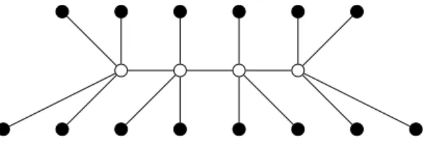
In the partner units problem, we are given a set of sensors grouped into zones. A sensor may be attached to several zones. Figure 3.1, for instance, shows a set of zones with 3 sensors attached to each of them. The goal is to connect the sensors and zones to a given number of control units and to define which pairs of control units are “partners,” so that two conditions are satisfied:

(i) if a sensor is attached to a zone, but the sensor and the zone are assigned to different control units, then these two control units are partners;

(ii) the number of sensors assigned to a unit, the number of zones assigned to a unit, and the number of partners of a unit do not exceed given upper bounds.

For example, the graph in Figure 3.2 shows a solution for the configuration in Figure 3.1 with 4 control units, assuming that each of the upper bounds (ii) equals 2. The horizontal edges represent the partnership relation between units.

A clingo program solving the partner units problem is shown in Listing 3.11, and Listing 3.12 is an input for that program corresponding to the example above.