Econometrics Lecture Notes – Fall 2012
Michael Malcolm
Unit 1: Introduction to Econometrics
Unit 2: Review of Probability and Statistics
2.1: Probability
2.2: Statistics
2.3: Hypothesis Testing and Confidence Intervals
Unit 3: Single-Variable OLS Regression
3.1: Estimation
3.2: Inference
3.3: Theoretical Properties
Unit 4: Multiple Regression
4.1: Estimation
4.2: Inference
4.3: Multicollinearity, Omitted Variables and Irrelevant Variables
4.4: Model Selection
Unit 5: Specification
5.1: Dummy Variables
5.2: Nonlinearities – Polynomial Expansions
5.3: Nonlinearities – Log Specifications
5.4: Nonlinearities – Interactions
Unit 6: Extensions and Modifications of OLS
6.1: Instrumental Variables – Motivation and Research Examples
6.2: Instrumental Variables – Estimation and Inference
6.3: Limited Dependent Variables
6.4: Panel Regression
Unit 7: Causal Inference
7.1: Causality
7.2: Validity
Unit 1: Introduction to Econometrics
Michael Malcolm
January 26, 2011
1
Origins and Nature of Econometrics
People often divide scholarly research into that which is theoretical and that which is empirical. Theoretical work uses deductive reasoning – it advances premises and then formulates conclusions that follow from the premises. By contrast, empirical work uses data to answer questions inductively – it is based on drawing generalizations from observation and evidence. Some scholars are fervent theorists or empiricists and view the two as being in conflict with each other. By contrast, the guiding theme of econometrics is that theory and empiricism can be complementary to each other. It’s good to have evidence and data to investigate theoretical claims, but it’s also important to have a strong enough grasp on theory to understand empirical evidence.
Econometrics is the application of statistical techniques to economic problems. The term seems to have been coined by Ragnar Frisch in 1933; what is important is that it emphasizes the unification of economic theory and empirical work. Econometrics encompasses both the development of techniques for analyzing data and the application of those techniques to actual data.
2
Framing Econometric Questions
An econometric question is typically framed as the response of one variable to changes in another variable. Here are a few examples of econometric research.
• What is the impact of income taxes on labor supply? (This question is particularly interesting because economic theory gives an ambiguous answer – higher tax rates could cause people to work more or to work less because the income and substitution effects pull in opposite directions.)
• How does rigorous enforcement of antitrust laws for doctors affect the quality of medical care? • Do pegged exchange rates lead to a more stable currency value?
Again, the key is that in all cases there is a nexus of theory and empiricism: between economic theory and analysis of data.
3
Econometrics and Statistics
Since its inception, econometrics has emphasized a few things that distinguish it from statistics, and in particular from the way in which other disciplines use statistics.
rather than a demand curve. This is a classic problem in econometrics and illustrates an important point: statistically, my analysis is perfectly valid. The problem is in the interpretation. Econometrics stresses that data alone is not enough – one needs to understand theory in order to make sense of data. • Econometrics emphasizes the need to choose the statistical model carefully depending on the nature of the problem. The most popular statistical model for studying the relationship between two variables is simple linear regression. The problem is that the linear model is inappropriate in many cases. Consider the relationship between education and wages – many people do not work at all and so their recorded wages are zero, which makes a simple linear relationship between wages and education inappropriate. As an example with macroeconomic data, GDP tends to grow exponentially rather than linearly. • Econometrics considers alternative explanations that could have generated the same statistical
relation-ship
– Suppose I want to study how much police presence lowers crime. When you look at the data and estimate the relationship, you may be surprised when you find that places with more police have more crime. Do police cause crime? Probably not – it seems more likely that high crime is the reason that lots of police are in these places. So we have two different explanations that would cause the same observed results. Whether police cause crime or whether high crime brings in more police, the statistical relationship is going to show that higher police presence is associated with more crime.
– Does graduating from a top-10 university raise wages? Statistically, it is unquestionable that people who graduate from higher-ranked schools earn higher wages. However, is attending a high-ranked school thecause of higher wages? People from top-ranked schools also have a higher IQ and come from wealthier families with more connections. Maybe the reason that people from top universities have higher wages is because of their higher IQs and more family connections, so that the degree itself is not thecause of higher wages. Again, we have two explanations that would both be consistent with the same data.
– People with friends who smoke are significantly more likely to start smoking themselves. Some might immediately see this as evidence of ”peer effects”. But there could be another explanation for the same results – maybe kids who are inclined to start smoking for whatever reason also tend to make friends with other kids who are inclined to start smoking. Again, either explanation would generate the same observed statistical relationship
In summary, there is a strong tradition of solid empirical work in economics. Not only are economists at the forefront of new techniques, but the discipline is well-known for being skeptical about the interpretation of statistical results. In the absence of theory, statistical results can easily be misleading and misinterpreted. There is a difference between thestatistical validity of a result and having a validinterpretationof the result.
4
Econometric Data
There are three types of data in econometrics.
• Cross-section data is data collected on multiple entities in a single time period. For example, I might conduct a survey of students and ask them about their GPAs, their gender and the number of hours that they sleep; each student is an entity. I might collect data on 2009 GDP per capita and 2009 immigration rates for many different countries; each country is an entity. These are both examples of cross-sectional data – the observations are different entities in the same time period.
• Panel data is data collected on multiple entities for multiple time periods. For example, I might survey the same people every year for 30 years about their income and their family status. I might collect data on governmental structure and economic growth for several years for many different countries. Here, multiple entities are each observed for multiple time periods.
While this is a generalization, microeconometrics tends to use more cross-section data and macroecono-metrics tends to use more time-series data. Panel data is used regularly by both. This class is more microeconometric and focuses on cross-section data, with some coverage of panel data towards the end. Economic forecasting deals more with macroeconometric data and covers time-series analysis in detail.
5
Different Kinds of Models
The simplest kind of statistical model of the relationship between two variables is the univariate linear model. We are interested in how Y responds to changes in X. Y is called the dependent variable or theleft-hand variable. Xis called theindependent variableor theright-hand variable. For example, we might be interested in how wagesY depend on educationX. If the relationship is linear, then we have the ”true model”:
Y =β0+β1X+u
So β0 is the intercept and β1 is the slope. Here,u is the error. There are probably other things that determineY besidesX, even if it’s just random noise.
The idea is to make many observations, which we index withi, and to collect many data points (xi, yi). For example, we ask many individuals i about their education levels and their wages. The idea of linear regression is to find the line that best fits the data points (we will talk about procedures and what is meant by ”best fit” later). See figure 1. We then have theestimated regression line:
ˆ
Y = ˆβ0+ ˆβ1X
It is important to note the difference betweenβ0andβ1, which are the intercept and slope from the true population regression line and ˆβ0 and ˆβ1, which are theestimated intercept and slope from the sample. The true population regression line is unobservable, whereas the estimated regression line is estimated from the sample.
In this case, ˆβ1 is the estimated slope – the change in Y resulting from a one-unit change inX. Note that this definitely does not say that an increase inX causes a change in Y. Using our earlier example, places with more police tend to have more crime, but it is wrong to interpret this to mean that increases in police presencecausecrime to rise.
One might also have a multivariate linear model, with many independent variables that are associated withY. For example, ifY is wage, thenX1=education,X2=age, X3=experience andX4=gender could all be factors that are associated with wages. The true population model is then:
Y =β0+β1X1+β2X2+β3X3+β4X4+u
Notice, for example, thatβ3is apartial effect. It is the estimated change in wage resulting from one more year of experiencewhile holding all other variables constant. We can use multiple regression to estimate the line that best fits the data and to obtain the estimated regression line:
ˆ
Figure 1: Fitting a regression line
Linear regression isn’t always the appropriate way to model the relationship between two variables. For example, the relationship between firm output and labor is nonlinear since it is subject to diminishing marginal returns. Education and economic growth tend to grow together exponentially, not linearly.
Unit 2.1: Probability Review
Michael Malcolm
January 26, 2011
1
Random Variables
Arandom variable is a numerical summary of a random outcome.
A discrete random variable takes on a discrete number of values. The number of accidents at an inter-sections, the outcome of the toss of a die or the gender of a baby (using, for example 0 for female and 1 for male) are all discrete random variables.
A continuous random variable takes on a continuum of values. Height or time spent waiting in line are continuous random variables.
2
Discrete Random Variables
Aprobability distribution describes the possible values of a random variable and the probability with which those values occur. For example, consider the random variable X measuring the number of children born to a pregnant woman. Standard notation is that capital X refers to the variable itself, while lower-casex refers to a realization of the variable. Here is an example of a probability distribution
x P r(X=x)
1 0.91
2 0.07
3 0.02
Theexpected value of a random variable is the average (mean) value of the variable across many trials. The expected value of the random variableX is denotedE(X) or with the Greek letterµ. The definition is:
E(X) =XP r(X=x)∗x For our example above:
E(X) = 0.91(1) + 0.07(2) + 0.02(3) = 1.11
So, on average, the number of children born to a pregnant woman is E(X) = 1.11.
The variance of a random variable is the expected value of the squared distance from the mean. The variance of a random variableX is denoted V ar(X). The definition is:
V ar(X) = 0.91(1−1.11)2+ 0.07(2−1.11)2+ 0.02(3−1.11)2 = 0.1379
Thestandard deviationof a random variable is the square root of its variance. The standard deviation of a random variableX is denotedsd(X). Alternatively, the Greek letterσis used for the standard deviation of a random variable, withσ2denoting its variance.
For our example above:
sd(X) =√0.1379 = 0.3713
3
Example: The Bernoulli Distribution
A frequently encountered discrete probability distribution is theBernoulli distribution. A Bernoulli random variable X is equal to 1 with probabilityp and is equal to 0 with probability 1−p. This is often used to describe qualitative outcomes; for example, a random variableX might be equal to 1 if a person is employed and 0 if a person is unemployed. Summarizing a Bernoulli random variable in the table below:
x P r(X=x)
0 1−p
1 p
A simple formula that describes the probability distribution is:
P r(X =x) =px(1−p)1−x To see why this formula holds:
P r(X = 1) =p1(1−p)1−1 =p
A similar calculation would give thatP r(X= 0) = 1−p. The mean of a Bernoulli random variable is:
E(X) =XP r(X =x)∗x = (1−p)∗0 + (p)∗1 =p
The variance of a Bernoulli random variable is computed as follows. Remember that E(X) = p for a Bernoulli variable.
V ar(X) =XP r(X =x)∗(x−E(X))2 = (1−p)(0−p)2+p(1−p)2 = (1−p)(p2) +p(1−2p+p2) =p2−p3+p−2p2+p3 =p−p2
Figure 1: Probabilities for a continuous random variable
For example, takeX= 1 for an employed person andX = 0 for an unemployed person. The probability of being employed isp= 0.75. Then the expected value and variance ofX are:
E(X) =p= 0.75
V ar(X) =p(1−p) = 0.1875
4
Continuous Random Variables
For a continuous random variable, the probability of any particular value is equal to 0. We can, however, describe probabilities over a range of outcomes. For example, the probability that a person’s height is 198.58373 cm exactly is zero. However, we could find the probability that a person’s height falls between 190 and 200 cm.
Probabilities for a continuous random variable are described with a probability density function, which we will denotef(x). For a discrete random variable, to find the probability that xtakes on certain values, we simply add the probability for each possible outcome. For example, to find the probability that there are 2 or 3 children born to a pregnant woman, we simply add upP r(X = 2) +P r(X= 3).
The analogue for finding probabilities associated with a continuous random variable is to integrate over the range of outcomes we’re interested in (since each individual outcome has zero probability). For example, the probability that height falls between x= 190 and x= 200 centimeters is shown in figure 1 – the area under the probability density function. We would calculate this asP r(190≤X ≤200) =R200
190 f(x)dx. Recall that the expected value (mean) of a discrete random variable is E(X) =PP r(X =x)∗x. The concept is the same for a continuous random variable except that we integrate rather than sum:
E(X) = Z
supp
f(x)∗x dx
Where the limits of the integration are determined by the range over which the range over which the random variable has a nonzero density. This is sometimes called thesupport of a random variable.
Figure 2: Probabilities for a continuous random variable
V ar(X) = Z
supp
f(x)∗(x−E(X))2dx
5
Example: The Exponential Distribution
The probability density function (pdf) for an exponential distribution is:
f(x) = 1 λe
−x λ
Here, λis a parameter of the distribution. xtakes on values from 0 to∞. The exponential distribution is used, among other things, to model waiting times and intensity of earthquakes.
For example, suppose that X measures the time waiting in line, which is modeled by an exponential distribution withλ= 5. Then the pdf of X is:
f(x) =1 5e
−x 5
Then the probability that you will wait in line for between 4 and 7 minutes is calculated as:
P r(4≤x≤7) = Z 7
4 1 5e
−x
5 dx= 0.203 This probability is shown in figure 2.
Using the formulae above, we can calculate the expected value for any exponential distribution:
E(X) = Z
supp
f(x)∗x dx
= Z ∞
0 1
λe −x
λ
And the variance:
V ar(X) = Z
supp
f(x)∗(x−E(X))2 dx
= Z ∞ 0 1 λe −x λ
∗(x−E(X))2 dx
= Z ∞ 0 1 λe −x λ
∗(x−λ)2 dx =λ2
6
Joint, Marginal and Conditional Distributions
Suppose thatX is a random variable measuring the number of children born to a woman andY is a random variable measuring the number of days that the woman stays in the hospital. We assume that each takes a value from the set{1,2,3}. The following table gives the joint probability distribution ofX andY. Notice that there are 9 possibilities. The probability thatX takes on the valuexand thatY takes on the valuey is denotedP r(X =x;Y =y) As usual, the probabilities must sum up to 1.
Y = 1 Y = 2 Y = 3
X = 1 0.83 0.07 0.01
X = 2 0.05 0.01 0.01
X = 3 0.01 0.005 0.005
Suppose that we have this table, but that we are interested only in the number of children born irrespective of hospital stay. Themarginal distributionofX is the probability thatXtakes on various values, irrespective of the value ofY. Formally, it is given by the formula:
P r(X=x) =X i
P r(X =x;Y =yi)
For example, the probability thatX is equal to 1 is 0.83 + 0.07 + 0.01 = 0.91 after adding up all the cases whereX = 1. The rest of the marginal distribution can be calculated similarly. The table below shows the marginal distribution ofX:
x P r(X=x)
1 0.91
2 0.07
3 0.02
Notice that this is given by the sums of the entries in therows of the joint probability distribution, since the rows account for the various values ofX.
Suppose instead that we are interested in the length of the hospital stay irrespective of the number of children born. The marginal distribution ofY is the probability thatY takes on certain values, irrespective of the value of X. For example, the probability thatY = 1 is 0.83 + 0.05 + 0.01 = 0.89, after summing up all the cases whereY = 1. Calculating other probabilities similarly, the marginal distribution ofY is:
y P r(Y =y)
1 0.89
2 0.085
Notice that this is given by the sums of the entries in the columns of the joint probability distribution. Suppose now that we are interested in the distribution of the hospital stay givena particular number of children. Theconditional distributionofY given thatX =xis the probability distribution ofY conditional on the random variableX being equal tox. This is denotedP r(Y =y|X =x) and is given by the formula:
P r(Y =y|X =x) = P r(Y =y;X=x) P r(X =x)
Where P r(X =x) denotes the marginal probability that X =x. For example, to find the conditional distribution ofY given thatX = 1 (i.e. the distribution of days in the hospital given that the woman who has one child).
P r(Y = 1|X = 1) = P r(Y = 1;X= 1) P r(X= 1) =
0.83
0.91 = 0.9121 P r(Y = 2|X = 1) = P r(Y = 2;X= 1)
P r(X= 1) = 0.07
0.91 = 0.0769 P r(Y = 3|X = 1) = P r(Y = 3;X= 1)
P r(X= 1) = 0.01
0.91 = 0.0110
However, the marginal distribution of Y conditional on X taking a value of 3 (i.e. the distribution of days in the hospital given that a woman has three children) is given by:
P r(Y = 1|X = 3) = P r(Y = 1;X = 3) P r(X = 3) =
0.01 0.02 = 0.5 P r(Y = 2|X = 3) = P r(Y = 2;X = 3)
P r(X = 3) = 0.005
0.02 = 0.25 P r(Y = 3|X = 3) = P r(Y = 3;X = 3)
P r(X = 3) = 0.005
0.02 = 0.25
We can compute conditional expectations and variances using a conditional distribution in the same way that we compute expected value and variance for any other distribution. For example:
E(Y|X = 1) =X i
P r(Y =yi|X =x)∗yi = 0.9121(1) + 0.0769(2) + 0.0110(3) = 1.0989
This is the expected number of days in the hospitalgiventhat a mother gave birth to one child. We can compute the conditional variance similarly:
V ar(Y|X = 1) =X i
P r(Y =yi|X =x)∗(yi−E(Y))2
7
Covariance and Correlation
The covariance between two random variablesX andY is defined as:
Cov(X, Y) =E[(X−E(X))(Y −E(Y))]
=X
i X
j
P r(X =xi;Y =yj)∗(xi−E(x))∗(yi−E(Y))
For our earlier example, E(X) = 1.11 and E(Y) = 1.135. So, using the joint distribution from the previous section,
Cov(X, Y) =0.83(1−1.11)(1−1.135) + 0.07(1−1.11)(2−1.135) + 0.01(1−1.11)(3−1.135)+ 0.05(2−1.11)(1−1.135) + 0.01(2−1.11)(2−1.135) + 0.01(2−1.11)(3−1.135)+ 0.01(3−1.11)(1−1.135) + 0.005(3−1.11)(2−1.135) + 0.005(3−1.11)(3−1.135) =0.045
Intuitively, if two random variables tend to move together, then they are more likely to fall above or below the mean jointly. In this case, the covariance between them will be positive. If both are above or below the mean, then the product (x−E(X))(y−E(Y)) is positive. Rainfall and crop yield are random variables with a positive covariance. One tends to be high when the other is high.
If one tends to be high (above the mean) while the other one is low (below the mean), then the product (x−E(X))(y −E(Y)) is negative. Random variables that are more likely to follow this pattern have a negative covariance with each other. Cigarette consumption during pregnancy and birthweight have a negative covariance. One tends to be low when the other is high.
The magnitude of the covariance is affected by the units chosen. By contrastcorrelation is a measure of the relation between two random variables that is unit-free. That is, the correlation between two variables is the same regardless of the units with which either variable is measured. The definition of correlation is:
Correl(X, Y) = p Cov(X, Y) V ar(X)V ar(Y) =
cov(X, Y) sd(X)sd(Y)
For our example,Cov(X, Y) = 0.045,V ar(X) = 0.1379 andV ar(Y) = 0.1668. Thus,
Correl(X, Y) =√ 0.045 0.1379∗0.1668 = 0.2967
This indicates a moderate direct relationship between the two. Correlations always lie between -1 and 1. A correlation close to 1 indicates a strong direct relationship – variables that move together (in fact, the correlation is exactly 1 when the relationship between the two is linear and positively sloping). A correlation close to -1 indicates a strong inverse relationship – variables where one tends to go up as the other goes down. A correlation close to 0 indicates two variables that do not have a strong linear relationship with each other.
8
Independence
P r(Y =y;X =x) =P r(Y =y)∗P r(X =x) Observe that this implies that:
P r(Y =y|X =x) = P r(Y =y;X=x) P r(X=x)
= P r(Y =y)∗P r(X=x) P r(X =x) =P r(Y =y)
What this means intuitively is that information about the value ofX tells us nothing about the value of Y. If P r(Y =y|X =x) =P r(Y =y), then knowing the value ofX doesn’t give us any information about the value ofY. Also, when two random variables are independent,Cov(X, Y) = 0 and soCorrel(X, Y) = 0.
As an example, suppose thatX andY had the marginal distributions shown below: x P r(X=x)
0 0.5
5 0.2
10 0.3
y P r(Y =y)
2 0.8
3 0.1
4 0.1
IfX andY are independent, then the joint distribution is:
Y = 4 Y = 5 Y = 6
X = 0 0.4 0.05 0.05
X = 5 0.16 0.02 0.02
X= 10 0.24 0.03 0.03
As illustrated by the definition of independence, the joint probability of any realization (xi, yi) is the product of the marginal probabilities ofxiandyi. Intuitively, knowing the marginal distributions is enough to construct the joint distribution.
Also, notice that the marginal probabilityP r(Y = 4) = 0.4 + 0.16 + 0.24 = 0.8. This should be equal to the conditional probability
P r(Y = 4|X = 0) = P r(Y = 4;X = 0) P r(X = 0) = 0.4
0.5 = 0.8
It is straightforward to show thatP r(Y = 4|X = 5) andP r(Y = 4|X = 10) are also equal to 0.8. Again, the intuition is that knowing the value of X tells you no additional information about the probability that Y takes on certain values – the two are independent of each other.
9
Transformations and Combinations of Random Variables
Suppose we have information about a random variableX but that we are interested in a transformation of X. For example, suppose thatX measures GDP in dirhams, but you want information on GDP in dollars. One thing you could do is to reconstruct the entire distribution and recalculate the mean and variance. Luckily, this is unnecessary – there are simple formulas for calculating the mean and variance of a variable that is a linear transformation of a variable for which the mean and variance are already known.
Suppose that we knowE(X) andV ar(X), but that we are interested in the transformed variablea+bX.
E(a+bX) =a+bE(X) V ar(a+bX) =b2V ar(X)
sd(a+bX) =b·sd(x)
Note that expected value is a linear operator. AS for variance, the parameterajust shifts the distribution, which doesn’t affect the variance. The parameterb rescales the variable, which does change the variance.
There are also formulas for combinations of random variables. Consider a random variable X with expected valueE(X) and varianceV ar(X) and a random variableY with expected valueE(Y) and variance V ar(Y). The covariance between the two isCov(X, Y).
Now suppose we are interested in a new random variable that is acombination of the two. For example, many economists study indices which combine many variables. Again, we could construct all possible values of the combined variable to calculate its mean and variance, but there are simple formulas that relate the properties of the combined variable with the known properties of the original variables.
E(a+bX+cY) =a+bE(X) +cE(Y)
V ar(a+bX+cY) =b2V ar(X) +c2V ar(Y) + 2bc·Cov(X, Y) E(XY) =E(X)E(Y) +Cov(X, Y)
Cov(a+bX, c+dY) =bd·Cov(X, Y)
An often-used special case of the first two formulas sets a= 0 andb=c= 1.
E(X+Y) =E(X) +E(Y)
V ar(X+Y) =V ar(X) +V ar(Y) + 2Cov(X, Y)
In particular, while the expected value ofX+Y is the sum of the expected value ofX and the expected value of Y, this is not generally true of the variance. The variance of X+Y also involves the covariance between the two. However, ifX andY are independent then theCov(X, Y) = 0 and so some of the formulas above simplify as follows. Again, note that the following holdonly ifX andY are independent:
Figure 3: P r(Z≤1)
10
The Normal Distribution
The most important and often-used distribution in econometrics is the normal distribution. The easiest way to find probabilities associated with the normal distribution is to use a table that tabulates these probabilities. A normal distribution is described by its mean and its standard deviation. We writeX ∼N(µ, σ) to denote
thatX is normally distributed with meanµand standard deviationσ. Normal distributions are symmetric, bell-shaped and centered around the mean. All normal random variables take on positive values from−∞to ∞, although the probability declines almost to zero if you move more than a couple of standard deviations away from the mean.
The standard normal distribution is the normal distribution with mean 1 and variance 0. A standard normal random variable is usually denoted Z so that Z ∼N(0,1). TheZ distribution is centered about 0 and is symmetric, so that probability 0.5 lies below 0 and probability 0.5 lies above 0. Tables that tabulate standard normal probabilities are easily available. They normally give the probability thatZ islower than a certain value z. For example P r(Z ≤ 1) = 0.8413 can be read directly from the table. The relevant probability is shown in figure 3.
To calculate P r(Z ≥0.83) using the table, observe that this is 1−P r(Z ≤ 0.83). This probability is illustrated in figure 4. Using the table:
P r(Z≥0.83) = 1−P r(Z ≤0.83) = 1−0.7967 = 0.2033
To calculate P r(−0.1≤Z ≤1.32), observe that this is P r(Z ≤1.32)−P r(Z ≤ −0.1). This probability is illustrated in figure 5. Using the table:
P r(−0.1≤Z ≤1.32) =P r(Z≤1.32)−P r(Z≤ −0.1) = 0.9066−0.4602
Figure 4: P r(Z ≥0.83)
An extremely useful property of the normal distribution is that any normal random variableX can be converted to a standard normal random variableZ using the following transformation:
Z =X−µ σ
In other words, calculating probability foranynormal random variable only requires knowing the standard normalN(0,1) distribution. For example, suppose thatX measures IQ score, which is normally distributed with mean 100 and standard deviation 15. Using our notation,X ∼N(100,15). To calculate any probability,
simply use the z-transformation above. For example:
P r(X ≥130) =P r
Z≥ 130−100 15
=P r(Z ≥2) = 0.0228 As another example:
P r(90≤Z≤110) =P r
90−100 15 ≤Z≤
110−100 15
=P r(−0.67≤Z≤0.67) = 0.4792
Sometimes we need to work with normal probabilities in reverse. For example, suppose we are interested in finding the value z0 such that P r(Z ≥ z0) = 0.10. We need to hunt on the z-table for the value of z0 such that 0.1 of the distribution lies to the right of z0 (i.e. where 0.9 lies to the left ofz0.) This occurs at z0= 1.28, i.e.
P r(Z ≥1.28) = 0.10 This probability is illustrated in figure 6.
As another example, suppose that we are interested in finding the IQ score x0 such that only 1% of students’ scores lie abovex0, i.e. P r(X ≥x0) = 0.01.
First observe from the z-table that:
P r(Z ≥2.33) = 0.01
Now, simply convert the relevant z-score back to the distribution of IQs X using the z-transformation:
Figure 6: P r(Z≥1.28) = 0.1
Unit 2.2: Statistics Review
Michael Malcolm
January 26, 2011
1
Sampling and Sample Statistics
Suppose that Y is a random variable describing a person’s height in centimeters. Each person’s height is randomly drawn from this distribution. This distribution can be described with the usual properties, with mean E(Y) = µ and variance V ar(Y) = σ2. Note that these are properties of the true population distribution and are generally unknown.
Statistics is about taking asampleand using this sample to draw inferences about the population. Taking a sample of sizenfrom the population, we denote our sample{y1, y2, ..., yn}. We typically assume that our sample isindependent andidentically distributed, often abbreviatediid.
• An independent sample means that knowing y1, for example, gives no information about any other member of the sample. One observed member of the sample is not dependent on any other member of the sample. If we sampled heights of fathers and sons, this might violate independence.
• An identically distributed sample means that all members of the sample are drawn from the same distribution. That is, before the observation is actually made, any member of the sample faces the same probability distribution of having various heights.
In econometrics, we virtually always assume that our samples are iid (Time-series data are an exception. For example, the unemployment rate in 2009 will typicallynot be independent of the 2008 unemployment rate).
Now, given an iid sample, we can construct statistics based on this sample. For example, the sample mean is:
Y = 1
n
n X
i=1
yi
Thesample variance is:
s2= 1
n
n X
i=1
(yi−Y)2
Thesample standard deviation is:
s= v u u t 1
n
n X
i=1
(For technical reasons, the sample variance and sample standard deviation are sometimes calculated using 1
n−1 instead of 1
n to normalize. Notice that if the sample sizenis large, it doesn’t make much of a difference). Suppose now that we have a paired sample, collecting both xi andyi from a sample with sizen. Then thesample covariance is:
sxy= 1
n
n X
i=1
(xi−X)(yi−Y)
And thesample correlation is:
r= sxy
sxsy
Sample statistics have the same transformation and combination properties as their population equiv-alents. For example, the sample mean is linear: if you double the value of each samples, then the sample mean doubles. However, if you multiply the value of each sample byb, then the sample variance is scaled up byb2.
2
Properties of Estimators
Suppose that we are using a sample statistic ˆθto estimate a population parameterθ. For example, we might be using the sample mean ¯Y to estimate the unknown population parameterµ. There are three desirable properties of such estimators:
• θˆis anunbiased estimator ofθifE(ˆθ) =θ. That is, the estimator – on average – is equal to the value of the parameter being estimated.
• θˆis aconsistent estimator ofθif ˆθ converges asymptotically toθas the sample size rises. That is, the estimator should get better and approach the true value of the parameter as the sample size rises.
• θˆis anefficient estimator ofθif ˆθhas the lowest variance among any possible unbiased estimator ofθ. Estimators are never perfect, and always have some variance around the true value of the parameter, but the efficient estimator is the one with thelowest variance among all unbiased estimators.
3
Properties of the Sample Mean
Consider using the sample mean ¯Y to estimate the true population meanµ. Let us calculate the expected value of ¯Y. Remember in doing this calculation that each member of the population is drawn from a population distribution whose mean height isµ.
E( ¯Y) =E
1
n(y1+y2+...+yn)
= 1
nE(y1) +
1
nE(y2) +...+
1
nE(yn)
= 1
nµ+
1
nµ+...+
Summarizing,E( ¯Y) =µ, meaning that – on average – the sample mean is equal to the population mean. Using the terminology just developed, ¯Y is anunbiased estimator of the population meanµ.
Now, let us calculate the variance of ¯Y.
V ar( ¯Y) =V ar
1
n(y1+y2+...+yn)
=V ar
1
ny1+
1
ny2+...+
1
nyn
=V ar
1
ny1
+V ar
1
ny2
+...+V ar
1
nyn
This last line follows only because the sample {y1, y2, ..., yn} is independent. Otherwise, the variance of this sum would also include covariance terms. In continuing with the calculation, recall that scaling random variables bybscales their variance byb2.
V ar( ¯Y) = 1
n2V ar(y1) + 1
n2V ar(y2) +...+ 1
n2V ar(yn)
Now, note that V ar(yi) =σ2 for all isince all members of the sample are drawn from the same distri-bution.
V ar( ¯Y) = 1
n2σ 2+ 1
n2σ
2+...+ 1
n2σ 2
= 1
n2(σ
2+σ2+...+σ2)
= 1
n2(nσ 2)
= σ 2
n
The key point is that, as the sample sizen increases, the variance of ¯Y falls. That is, the sample mean tends to bunch up around the population mean with less variance in the possible values that ¯Y could take. If the sample size is small, there is lots of variance in the sample mean – although itsexpected value is equal to the population mean, there is a lot of dispersion in the values ¯Y could take. However, as the sample size gets larger, this variance falls and ¯Y collapses to its expected value ofµ.
In fact, the variance falls to 0 as the sample size rises. This means that ¯Y is aconsistent estimator ofµ. ¯
Y approachesµ asymptotically as the sample size rises. The result that ¯Y is a consistent estimator ofµis known as theweak law of large numbers (WLLN).
Although we will not prove it here, it turns out that ¯Y is also theefficient estimator ofµ. That is, there is no other unbiased estimator ofµwith a lower variance.
In summary, the sample mean ¯Y is an unbiased, consistent and efficient estimator of the population mean
µ.
4
The Central Limit Theorem
Figure 1: Distribution of Sample mean forn= 50 andn= 500
Thecentral limit theorem (CLT) states that, as the sample size increases, the distribution of the sample mean approaches a normal distribution with meanµand standard deviation √σ
n. With notation:
Y →N
µ,√σ
n
Intuitively, the distribution of ¯Y is always centered correctly around µ, with the distribution getting tighter (i.e. a smaller variance) as the sample size rises. Note that this is an asymptotic limit result and the approximation is only good if the sample sizenis reasonably large. This is hardly ever an issue in economics, but can be an issue in other disciplines where it is routine to use very small sample sizes.
Consider a population where the true mean isµ= 7. Figure 1 shows the distribution of the sample mean ¯
Y when the sample size isn= 50 and also when the sample size is n= 500. The distribution is centered correctly in either case, but there is much more dispersion when the sample size is lower. The variance shrinks as the sample size rises.
The amazing thing about the central limit theorem is that it holds regardless of the population distribu-tion. That is, no matter what kind of distribution the original population comes from – it might be discrete or heavily skewed – the distribution of a sample mean drawn from this population always approaches a normal distribution.
5
Using the Central Limit Theorem: Example 1
Consider a random variable measuring birthweightsY. Birthweights are not normally distributed; they are skewed left because of premature births. Suppose that the mean birthweight is µ = 7 and the standard deviation of birthweights isσ= 2. Figure 2 shows the distribution of birthweights.
Although the distribution of birthweights is not normal, the distribution of thesample mean taken from a sample of birthweights is approximately normal, according to the central limit theorem.
For example, suppose that the sample size is n= 30 and we are interested in the probability that the average birthweight in this sample exceeds 7.5 pounds, i.e. P r( ¯Y ≥ 7.5). According to the central limit theorem, ¯Y is normally distributed with mean 7 and standard deviation √2
Figure 2: Left-Skewed Distribution of Birthweights
P r( ¯Y ≥7.5) =P r Z ≥7.52−7 √
30 !
=P r(Z≥1.37) = 0.0853
Now suppose instead that we take a sample size ofn= 100, then according to the central limit theorem, the sample mean ¯Y is normally distributed with mean 7 and standard deviation √2
100. In this case:
P r( ¯Y ≥7.5) =P r Z ≥7.52−7 √
100 !
=P r(Z≥2.50) = 0.0062
As the sample size rises, the sample mean is more likely to be around the true mean µ= 7. Thus, the probability that the sample mean will exceed 7.5 falls as the sample size gets larger.
6
Using the Central Limit Theorem: Example 2
Consider a Bernoulli random variable Y that equals 1 for a smoker and 0 for a nonsmoker. This random variable is certainly not normally distributed since the only possible values it can take are 0 or 1. However, the central limit theorem tells us that asample meantaken from this distribution will be normally distributed – it will be centered around the true population mean, with a normal distribution around this mean, and collapsing variance as the sample size rises.
Suppose that the probability P r(Y = 1) = 0.4 for any member of the population. Recall from our discussion of Bernoulli random variables in the previous unit that the mean value ofY isµ=p= 0.4. The variance ofY isσ2=p(1−p) = 0.4(1−0.4) = 0.24, so that the standard deviation ofY isσ=√0.24 = 0.49.
Suppose we take a sample n= 100. The CLT tells us that ¯Y is distributed N(0.4,√0.49
100). So if we are interested in finding the probability that more than 0.3 of our sample are smokers:
P r( ¯Y ≥0.3) =P r Z≥ 0.30.49−0.4 √
100 !
Figure 3: n= 5
7
Simulating the Central Limit Theorem
A good way to check large-sample results generally is to simulate a large number of random samples and determine whether their properties obey what theory would predict. Consider the following random variable
X:
x P r(X=x) 0 0.92 1 0.005 2 0.005 3 0.005 4 0.005 5 0.005 6 0.005 7 0.005 8 0.005 9 0.04
It is straightforward to calculate that E(X) = 0.54. Notice that this is not even close to a normal distribution. Not only is it discrete, but it is heavily skewed. However, the central limit theorem tells us that, as long as the sample size is sufficiently large, that thesample mean should be approximately normally distributed around a meanµ= 0.54. That is, if we take a sample mean many times, the sampling distribution should be centered around 0.54 and with an approximately normal distribution about this mean.
First, let’s try n = 5. We create 1000 random samples from the distribution of X, with each sample consisting of 5 observations. Now we calculate the sample mean of each of the 1000 samples. Figure 3 shows the distribution of those sample means. It’s not even close to normal – clearlyn= 5 is not a large enough sample to apply the central limit theorem.
Let us now try a bunch of samples withn= 25. Again, we simulate 1000 samples with n= 25 in each sample. Figure 4 shows the distribution of those sample means. It’s still pretty asymmetric, with a long right tail.
Increasing the sample size ton= 100, we again simulate 1000 samples. Taking the sample mean of each of these samples, the distribution is closer to normal. It is shown in figure 5.
Figure 4: n= 25
Figure 6: n= 800
Unit 2.3: Hypothesis Testing and Confidence Intervals
Michael Malcolm
January 26, 2011
1
Principle of Hypothesis Testing
The principle of hypothesis testing is to start with a null hypothesis (denoted H0) and an alternative hy-pothesis (denoted Ha). The null hypothesis is what is assumed to be true before the test, whereas the alternative hypothesis is normally what the researcher is investigating or trying to find evidence for. For example, suppose that the average IQ in a school is 110, but a researcher is investigating whether smaller class sizes raise IQ test scores. Then the null is the starting supposition that the average IQ in the smaller class sizes is still 110, whereas the alternative is that average IQ is higher than 110. The null hypothesis in a trial is that the accused person is innocent. The alternative hypothesis is that the accused person is guilty – which is what the prosecutor tries to assemble evidence to demonstrate.
Hypothesis testing then applies a pre-specified test, typically using available data, to determine whether or not the null hypothesis is rejected in favor of the alternative hypothesis. A note on terminology: statisticians do not refer to ”accepting” the null hypothesis. If there is not enough evidence to rejectH0in favor ofHa, then we are not technically acceptingH0, but rather finding that there is not sufficient evidence to reject it. With this in mind, the chart below shows the results of the hypothesis tests and the corresponding ”true” state of the world, which is unknown.
True State: H0 is false True State: H0 is true
Test Result: RejectH0 Correct Result Type I error
Test Result: Do not RejectH0 Type II error Correct result
IfH0 is false and our test rejectsH0or ifH0is true and our test does not rejectH0, then the hypothesis test has reached the correct result.
2
Size and Power
If the true state of the world is that H0 is true, but our test rejectsH0 anyway, this is known as a Type I error. The probability of a type I error, usually denotedα, is known as thesizeof the test.
Size =P r(Type I Error) =α
The size is the probability of rejecting H0 when it is actually true. The ideal size for a test isα= 0. By contrast, if the true state of the world is that H0 is false, but our test does not reject H0, this is known as aType II error. The power of a test, usually denotedβ, is the probability of rejectingH0when it is false. Thus, the power is 1−P r(Type II Error).
Power = 1−P r(Type II Error) =β
There is generally a tradeoff between size and power. Suppose that the null is that average IQ is 110 but you are investigating the alternative that a new program raised IQ above 110. Suppose that your test is extremely strict, for example you don’t reject the null hypothesis unless the sample mean IQ in the classroom is greater than 150. It is highly unlikely that the null is true but that the sample mean IQ will be higher than 150. Thus, the size of this test is very close to 0. The problem is that, even ifH0 is false, it would be very difficulty to reject it with such a strict test. The power of this test is quite low.
On the other hand, suppose that we had a less strict test: we will reject the null as long as the sample mean in the classroom is higher than 112. In this case, there is a large risk that – even ifH0is true and the mean IQ is actually 110 – that we will rejectH0anyway because of random sampling issues. In other words, even if mean IQ is actually 110, it is not too unlikely that our sample mean may end up being higher than 112 just because of random sampling. In other words, the size of this test is rather high. Even when H0 is true, there is a high probability of rejecting it anyway. By contrast, the power of the test is quite high – if
H0 is false and the mean IQ is actually higher than 110, then it will be rather easy for our test to pick this up.
A strict test for rejectingH0has a low size but also has a low power. An test that makes it easy to reject
H0will have a high power, but also has a high size. The generally accepted method of resolving this tradeoff is to set the size at an acceptable level (oftenα= 0.05) and then use the test with the highest possible power given this size.
3
Statistical Logic of Hypothesis Testing
Hypothesis testing is basically just an application of the central limit theorem. The way hypothesis tests work in general is that we begin by assuming that the null hypothesis is true. For example, we assume that the true mean IQ in the classes with a smaller number of students isµ= 110. If this is true then, according to the central limit theorem, thesample meanfollows an approximately normal distribution centered around 110 and with standard deviation √σ
n. If the observed sample mean that we obtain is very unlikely under this distribution, then we reject the null hypothesis.
Graphically, see figure 1. This is the distribution of ¯xwhen the true population mean isµ= 110. The shaded region is the rejection region – if the observed sample mean is highly unlikely (usually probability less than 0.05) under the null hypothesis, then we will reject the null hypothesis. Notice that the probability associated with the rejection region is exactly the size of the test. When the null hypothesis is true, there is a probability 0.05 that the sample mean will fall in the rejection region, and thus that we will incorrectly reject the null.
Using the z-transformation, we usually express rejection regions in terms of z-statistics. For example, we know that there is a 0.05 probability that a z-statistic will exceed 1.64. Thus, in terms of z-statistics, the rejection region corresponding to the problem above isz > 1.64. See figure 2. Using the central limit theorem, ¯xis normally distributed with meanµand standard deviation √σ
n, so the relevant z-statistic is:
z= x¯−σ µ √
n
The specific steps to follow in constructing a hypothesis test are:
1. Set up the hypotheses.
2. Formulate the rejection region.
3. Calculate the test statistic.
Figure 1: Distribution of sample mean underH0 with rejection region
One important point. The hypotheses are always a function of unknown population parameters – the true meanµfor example. It is very wrong to state hypotheses in terms of sample statistics like ¯xbecause these are known statistics based on the data; there is nothing to hypothesize about.
4
Finding One-sided Rejection Regions
For a rejection region with 5% probability, we need z > 1.64. Using the normal table, the probability associated with this is 0.05, as desired. A standard notation isz0.05 = 1.64, meaning that 0.05 probability of the normal distribution falls to the right of 1.64.
A systematic way to go about finding these cutoff values is to use the ∞line of the t-table commonly available in statistics books. For a test with a 10% significance level (i.e. the size is 10%, meaning a 10% probability of falling into the rejection region under the null), the rejection region would bez >1.28. But for a test with a 1% significance level, the rejection region would bez >2.33. Alternatively,z0.1= 1.28 and
z0.01= 2.33.
If we were interested in the alternative that the mean is lower than some hypothesized value, then – since the normal distribution is symmetric – the rejection region for a 5% test would bez <−1.64 and for a 1% test would bez <−2.33, for example.
5
Hypothesis Test: Example 1
We are testing whether smaller class sizes raise average IQ above the assumed null valueµ= 110. We take a random sample ofn = 64 students and find that the sample mean IQ among these students is ¯x= 112 with a standard deviations= 9.3.
We want to test these hypotheses with a sizeα= 0.05.
1. Hypotheses H0:µ= 110
Ha:µ >110.
2. Rejection Region
RR:z >1.64
3. Test Statistic z= ¯x−µ√σ
n
= 112−110√9.3 64
= 1.72
4. Conclusion
Sincez >1.64, we reject the null hypothesis.
Since the test statistic falls in the rejection region, we reject the null hypothesis in favor of the alternative hypothesisµ >110.
6
P-Values
Thep-value is the lowest significance levelαfor which the null hypothesisH0would have been rejected. For the previous example, with our test statisticz= 1.72, note from the normal table thatP r(z >1.72) = 0.0427. This is the p-value.
Figure 3: 5% rejection region for a two-sided test
lowest significance level for which the null hypothesis can be rejected. We can reject the null for significance levels greater than 0.0427 and will not reject for significance levels less than 0.0427.
Another way to think about the p-value is that it is the probability of obtaining a sample mean of 112 or higher when the null hypothesis is true. That is, ifH0were true, and the mean IQ were reallyµ= 112, then we would only observe a sample mean IQ this high or higher 4.27% of the time, which is rather unlikely.
When the p-value is low, it is less likely to obtain the result under H0. In other words, it is more likely thatH0is false. Thus, we reject the null hypothesis for low p-values.
7
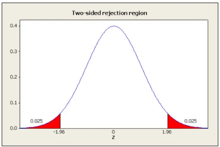
Two-Tailed Tests (two-sided tests)
Suppose that we have a hypothesized null value, but we are unsure about the direction of the alternative. We want to reject the null if the sample mean is significantly higheror lower than the hypothesized value. For a 5% rejection region, this would mean that we need 2.5% probability in each of the two tails. Again using the ∞line of the t-table corresponding to two-sided tests, the rejection region isz >1.96 andz <−1.96, which gives 5% probability. This is shown in figure 3. Using the notation from earlier, the 5% rejection region for a two tailed test isz > z0.025 orz <−z0.025.
8
Hypothesis Test: Example 2
We are interested in whether a new set of school policies has changed the number of days that students are absent. The null is that the true mean is equal to the hypothesized value ofµ= 10. We are interested in the alternative that the mean is loweror higher than this, i.e. a two-sided alternative.
We samplen= 50 students and find a sample mean ¯x= 12.3 and a standard deviations= 12.44.
1. Hypotheses H0:µ= 10
Ha:µ6= 10
2. Rejection Region
Figure 4: p-value = 0.1902 for a two-sided test
3. Test Statistic z= ¯x−µ√σ
n
= 12.3−1012.44√ 50
= 1.31
4. Conclusion
Since the test statistic does not fall in the rejection region, we do not rejectH0.
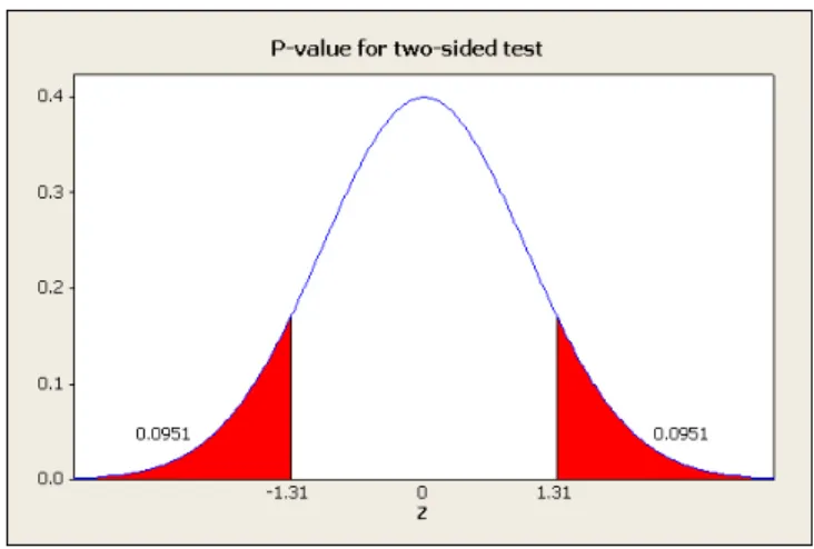
Now, the test statistic isz= 1.31 andP r(z >1.31) = 0.0951. However, notice that to reject, we would have needed this probability in both tails since it is a two-sided test. Thus, the p-value is twice this, or
p= 0.1902. See figure 4.
This means that the null hypothesis can only be rejected at significance levels above 19.02%. In other words, we cannot rejectH0at conventional significance levels like 1% or 5%. The way to think about this is that, ifH0were true, we would observe a sample mean this far or farther from the hypothesized value 19.02% of the time anyway. Thus, this is not very good evidence in favor of rejectingH0. We cannot conclude that
H0 is false with these data.
9
Hypothesis Test: Example 3
We can test hypotheses involving proportions using exactly the same logic. Just remember that the standard deviation isσ =pp(1−p) using results from unit 2.1. Thus, if the true population proportion is pthen, according to the central limit theorem, the sample proportion ˆpis normally distributed with mean p and standard deviation
√ p(1−p)
√
n . The appropriate z-statistic, therefore, is:
z= √pˆ−p p(1−p)
√ n
A new smoking prevention program has been initiated among n = 200 students. The null is that the proportion who become smokers isp= 0.2. The researcher is investigating the alternative that the program results in lower smoking rates. Among the sample 36 students, or ˆp= 0.18 become smokers. We want to test the hypothesis at a 5% significance level.
H0:p= 0.2
Ha:p <0.2
2. Rejection Region
RR:z <−1.64
3. Test Statistic z= √p−pˆ
p(1−p) √
n
= √0.18−0.2 0.2(1−0.2)
√ 200
=−0.71
4. Conclusion
Since the test statistic does not fall in the rejection region, we do not rejectH0.
10
Power of Tests (Sensitivity)
Thesize of a test is the probability of rejecting the H0 whenH0 is true. The sizeαis set before the test. 5% is a typical size.
Thepower of a test is the probability of rejectingH0 whenH0 is false. For example, if our null is that mean IQ is µ= 110 but the reality is that the mean IQ has risen has risen toµ >110, then the power is the probability that we will be able to reject the null hypothesis. As such, the power depends on how farµ
has risen. If the true mean IQ has risen toµ= 111, thenH0is false and we should reject it but – unless the sample size is very large – it will probably be difficult to pick up a difference this small. On the other hand, if IQ has risen toµ= 140, then the power of the test will be quite large – it will be easier to reject the null thatµ= 110.
11
Calculating Power for Example 1
To calculate power, we need to first find the rejection region explicitly in terms of the sample mean ¯x. For example 1, the rejection region was:
z >1.64 ¯
x−110 9.3 √
64
>1.64
¯
x >111.91
The power, then is the probability that the sample mean will fall in this rejection region for a particular value of µ. Suppose that the mean IQ has risen to µ = 113, so that the null is false. The power is the probability that the sample mean will fall into the rejection region whenµ= 113. Using the central limit theorem:
P r(¯x >111.91|µ= 113) =P r z > 111.919.3−113
√ 64
!
=P r(z >−0.94) = 0.8264
What if, however, the mean IQ had risen toµ= 130? Then the probability of falling into the rejection region is:
P r(¯x >111.91|µ= 130) =P r z > 111.919.3−130
√ 64
!
=P r(z >−15.56) ≈1
If true IQ has risen toµ= 113, then the probability that our test will reject the null thatµ= 110 is only 0.8264. However, if true IQ has risen toµ= 130, then it is virtually certain that our test is sensitive enough to pick this up; the power is nearly 1.
12
Calculating Power for Example 2
The rejection region contains two tails in this example. Calculating it explicitly, the rejection region is:
z <−1.96 orz >1.96
⇒x¯12.44−10 √
50
<−1.96 or x¯12.44−10 √
50
>1.96
⇒¯x <6.55 or ¯x >13.45
Suppose that the true mean days of absence has fallen toµ= 8. Then the probability of falling into the rejection region (i.e. the power of the test) is:
P r(¯x <6.55|µ= 8) +P r(¯x >13.45|µ= 8)
=P r z < 6.5512.44−8
√ 50
!
+P r z > 13.12.4445−8
√ 50
!
=P r(z <−0.82) +P r(z >3.10) = 0.2061 + 0 = 0.2061
In other words, even if the true mean has fallen toµ= 8, the probability of rejecting the null hypothesis is only 0.2061 under these circumstances. The only real solution here is to raise the sample size.
13
Confidence Intervals
We want an interval that contains µ with probability 1−α. Using notation from earlier, 1−α of the z-distribution falls between−zα
2 andz α
2. For example, since 2.5% falls above 1.96 and below -1.96, it follows that 95% of the z-distribution is contained in−zα
P r −zα
2 ≤z≤zα2
= 1−α
P r −zα 2 ≤
¯
x−µ
s √ n
≤zα 2
!
= 1−α
P r
¯
x−zα 2
s
√
n ≤µ≤x¯+zα2
s
√
n
= 1−α
Therefore, the following interval contains µwith probability 1−α
¯
x−zα 2
s
√
n,x¯+zα2
s
√
n
Statistical puritans would say that a more correct way to say this is that, in repeated sampling, this confidence interval would containµin fraction 1−αof the samples.
Since z0.025 = 1.96, a 95% confidence interval for µ is therefore h
¯
x−1.96√s
n,x¯+ 1.96 s √ n
i
. And since
z0.005 = 2.58, a 99% confidence interval for µ is h
¯
x−2.58√s
n,x¯+ 2.58 s √ n
i
. Importantly, as the confidence level rises, the interval becomes wider. If we want to be more certain thatµis contained within the interval, we are not going to be able to give as tight of an interval.
There is a connection between hypothesis tests and confidence intervals. Using the data from example 2 above, a 95% confidence interval for the true meanµis:
¯
x−1.96√s
n,x¯+ 1.96 s √ n =
12.3−1.96 12.44
√ 50
,12.3 + 1.96 12.44
√ 50
= [8.85,15.75]
Since the 95% confidence interval containsµ= 10, then we cannot reject the null hypothesis thatµ= 10. In other words, given our data, with 95% confidence it is possible that the mean isµ= 10.
Confidence intervals for proportions are almost the same. Simply replace the standard deviation with the appropriate standard deviation for a binary random variable. A 1−αconfidence interval is, therefore:
" ˆ
p−zα 2
p ˆ
p(1−pˆ) √
n ,pˆ+zα2 p
ˆ
p(1−pˆ) √
n
#
14
Simulating the Size of a Hypothesis Test
Generate 10,000 samples of size 100 from a random variable that has meanµ= 0.5. For each of the 10,000 samples, compute the mean and standard deviation.
Now suppose that we construct a hypothesis test for the null that µ= 0.5. Compute the z-statistic for each of the 10,000 samples:
z= x¯−s0.5 √
100
Unit 3.1: Single-Variable OLS Regression – Estimation
Michael Malcolm
January 26, 2011
1
Terminology and Setup
For single-variable linear regression, we are interested in the relationship between adependent variableyand anindependent variable x. For example, we might be interested in the relationship betweeny = wage and x= education. Here, there should be a direct relationship – increases in xare associated with increases in y. Or we might be interested in the relationship betweeny= unemployment andx= GDP. Here, we would expect an inverse relationship – increases inxare associated with decreases iny.
In linear regression, the true population relationship betweeny andxis linear. Specifically,y is a linear function ofx.
yi=β0+β1xi+ui
This is known as thepopulation regression line.
• i= 1, ..., ndenotes a member of the population.
• yi is the dependent variable, also called theregressand or theleft-hand variable
• xi is the independent variable, also called theregressor or theright-hand variable
• β0 is the intercept. If y is wage and x is education, then it represents the expected wage with no education.
• β1is theslope. This is the change inyresulting from a 1-unit increase inx. Mathematically, we could write this as dyi
dxi. Whenyis wage andxis education, then it represents the expected increase in wage
associated with one more year of education.
• uiis theerror. In general, other things determineyi besidesxi. It is possible that two people with the
same educationximight have different wagesyi. Some of these other factors might be age, experience,
gender, location or even just random noise.
Importantly, β0 andβ1 are the parameters of the true population regression line. These are unknown. We are trying to estimate them. This is like estimating the population mean – the true population meanµ is an unknown parameter, and ¯xis an estimator.
2
Estimating
β
0and
β
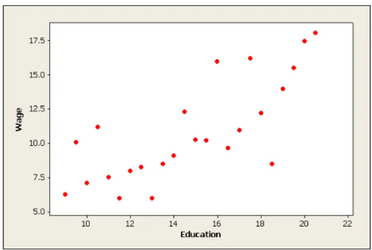
1Suppose that we have a random sample consisting ofn observations of the pair (xi, yi). The scatterplot is
shown in figure 1.
Figure 1: Random sample of data on education and wages
Figure 2: Regression residuals ˆui
ˆ
yi= ˆβ0+ ˆβ1xi
Theresidual uˆi is the difference between the true value of yand the value ˆy predicted by the regression
line.
ˆ
ui=yi−yˆi
Unless the data fit perfectly onto a straight line, there will always be some residual. Figure 2 shows a proposed regression line along with the residual for two observations. Observe that the residual can be positive, if the true yi is above that predicted by the regression line, or it can also be negative, when the
trueyi is below the value predicted by the regression line.
It is very important to be clear on the distinction between the residual ˆui and the errorui The error is
Now, in estimating ˆβ0and ˆβ1, we want to find an estimated regression line that keeps the residuals as low as possible. Obviously, if we just added the residuals, the positives and negatives would cancel. Thus, our objective is to minimize the sum of thesquared residuals. That is, for each observation, we take the square of the difference between the actual yi and the ˆyi predicted by the regression. We then sum the squared
residuals for each observation. The sum of squared residuals is:
SSR=
n
X
i=1
(yi−yˆi)
2
Now, the predicted ˆyi is determined by the estimated regression line ˆyi= ˆβ0+ ˆβ1xi.
SSR=
n
X
i=1
yi−
ˆ
β0+ ˆβ1xi
2
The ordinary least squares (OLS) estimates ˆβ0 and ˆβ1 are those that minimize the sum of the squared residuals. The problem is to choose the ˆβ0 and ˆβ1 that solve:
min
n
X
i=1
yi−β0ˆ −β1xˆ i
2
To solve this minimization problem, take derivatives with respect to ˆβ0 and ˆβ1and set them equal to 0.
∂SSR
∂βˆ0 =−2
n
X
i=1
yi−β0ˆ −β1xˆ i
= 0
∂SSR
∂β1ˆ =−2
n
X
i=1 xi
yi−βˆ0−βˆ1xi
= 0
This is two equations in two variables. After some algebra, one can solve these equations for ˆβ0 and ˆβ1.
ˆ β1=
1
n
Pn
i=1(xi−x) (y¯ i−y)¯
1
n
Pn
i=1(xi−x)¯
2
ˆ
β0= ¯y−βˆ1x¯
Notice that the numerator of our estimator ˆβ1 is just the sample covariance between xand y, and the denominator is the sample variance ofx. Thus, an even cleaner way to write the estimator is:
ˆ β1=
sxy
s2
x
The slope of the true population regression line would be β1= σxy
σ2
x. But the true population covariance
3
Numerical Properties of the Regression Line
Estimating ˆβ0 and ˆβ1 using the OLS formulation above, then the predicted value ofyi, given xi is:
ˆ
yi= ˆβ0+ ˆβ1xi
The residual is the difference between the actual value ofyiand the value ofyipredicted by the regression
line:
ˆ
ui=yi−yˆi
There are a few numerical properties of the estimated regression line and residuals that hold by definition.
1. Pn
i=1uˆi = 0. In words, the positive and negative residuals cancel each other out. If you sum up the
residuals under the OLS regression line, they always sum to 0.
2. Pn
i=1uˆixi= 0
3. The regression line passes through (¯x,y).¯
To see why these hold, recall from the previous section the first-order conditions for the minimization problem:
∂SSR
∂β0ˆ =−2
n
X
i=1
yi−β0ˆ −β1xˆ i
= 0
∂SSR
∂βˆ1 =−2 n X i=1 xi
yi−β0ˆ −β1xˆ i
= 0
Dividing both sides by−2 and substituting in the definition ˆyi= ˆβ0+ ˆβ1xi.
n
X
i=1
(yi−yˆi) = 0
n
X
i=1
xi(yi−yˆi) = 0
Butyi−yˆi is just the residual ˆui.
n
X
i=1 ˆ ui= 0
n
X
i=1
xiuˆi= 0
This verifies properties (1) and (2) above. They just come from the first-order conditions of the OLS minimization problem. These two equations are sometimes called thenormal equations.
ˆ
β0= ¯y−β1ˆ x¯
Rearranging this expression:
¯
y= ˆβ0+ ˆβ1x¯
In other words, (¯x,y) is on the OLS regression line.¯
4
Goodness of Fit
R2 is the percentage of variation in y that is explained by x. For example, we know that there is some variation in wagesy. What percentage of this variation is explained by differences in educationx?
Thetotal sum of squares (TSS) is the total (squared) variation inyabout its mean.
T SS=
n
X
i=1
(yi−y)¯ 2
Theexplained sum of squares (ESS) is the variation about ¯y explained by the regression line.
ESS=
n
X
i=1
(ˆyi−y)¯
2
Then the proportion of the variation iny explained by the regression line is:
R2= ESS T SS
Note that R2 always falls between 0 and 1. R2 = 1 if the data fit on a perfectly straight line, when the regression line explains all the variation in y. R2 = 0 is the regression line cannot explain any of the variation iny.
To expand this idea further, recall that the sum of squared residuals (SSR) is the sum of the squares of the residuals – the difference between the actualyi and the ˆyi predicted by the regression line.
SSR=
n
X
i=1
(yi−yˆi)
2
The following identity gives the relationship between the three:
T SS=ESS+SSR
The way to interpret this is thatT SSrepresents all of the variation iny. ESS is the part of the variation that is explained by x, while SSR is the part of the variation that is not explained by the regression line. Using the formula above, it follows then that an alternative way to write outR2is:
R2=T SS−SSR T SS = 1−
SSR T SS
Another numerical property is thatR2 is actually the square of the sample correlation betweenxandy.