Mathematical Modeling of One Wheel Robot Stabilized by Reaction Wheel Principle using Kane’s Method

(1)

3740

Abstract— One wheel robot was developed for the first time

by IIT technocrats. various principles have been applied till date to stabilized the one wheel robot, such as Gyrover, Gyrobot, etc. few researchers was developed Mathematical modeling of one wheel robot through Lagrangian constrained generalized formulation.

In this work, mathematical modeling of a OWR which is subjected to nonholomics constrains was derived by using Kane’s method. The movement OWR balance through reaction wheel principle, the assumption made while deriving equations of motion is that robot moves on level (flat) surface without slipping. Numerical simulation has also been presented to behavior of robot with different initial condition.

Index Terms— Kane’s method. OWR-One Wheel Robot,

INTRODUCTION

One wheel Robot which is also called Rectobot is class of portable robot. It is an enclosed single-wheel robot with an internal reaction wheel which gives mechanical stabilization and guiding capability. The robot is balanced by inciting an internal reaction wheel suspended from the focal point. By pitching the suspended mass inside the wheel forward or in reverse, the robot can be made to accelerate forward and backward, respectively. Turns are executed by tilting the robot to one side while it is in movement.

Fig.1: Solidworks Model of OWR

Since most recent two decades, huge numbers of specialists are working over wheeled mobile robot. They have watched that numerous wheeled vehicles gives great

static security keeping gravity vector through its focal point of mass inside the polygon of support. But during dynamic locomotion, latency powers get to be noteworthy as compare with gravitational powers. At higher rates dynamic aggravations particularly in rough territory get to be huge. More measure of vitality data is needed for controlling system momentum. Regularly endeavor to increase static stability causes dynamic insecurity in such circumstances. Consider the case of four wheel vehicle. It has wide polygon of bolster and is statically steady. Yet, when it disregards knocks, dynamic unsettling influence in the driver's seat makes expansive torque to topple the vehicle. Along these lines, dynamic stability is an imperative issue in fast portable robots. Dynamic stability requires effective absorption of energy and can be improved by properly designed vehicle suspension. Consider another case, for example, a bike It is statically unsteady in move heading. However, it has great element strength at fast, with gyroscopic activity and fitting directing of front wheel. Controlling strength increments with velocity because of the gyroscopic impact. An element power in the driver’s seat ground contact point follow up on or close to the sagittal (vertical) plane, in this way delivers huge move unsettling influences. Likewise, bikes can stay upright when going on slants and it can consequently change itself. Bicycle with static instability has good dynamic stability.

OWR uses the reaction wheel inverted pendulum concept for stabilization. Reaction wheel is driven by a motor. Forward/backward motion is implemented by another motor mounted within the wheel. Steering of wheel can be done by changing roll and pitch movements of the wheel. There are several motivations for developing a one wheel robot such as the OWR. First, this construction allows the robot to travel over obstacles more easily than other vehicles of similar size. Second, this entire structure is enclosed within one shell and there are no protruding parts outside the shell. If the seals are made watertight then we may be able to use this robot on wet surfaces. Full drive traction is available because all the weight is on the single drive wheel. Finally, dynamically stabilizing this unusual system is an interested problem in itself.

KANE’S METHOD

Basically all techniques for acquiring mathematical statements of movement are proportional. Then again, the usability of the different techniques varies; some are more suited for multibody elements than others. The Newton-Euler strategy is thorough in that a complete answer for

Mathematical Modeling of One Wheel Robot

Stabilized by Reaction Wheel Principle using

Kane’s Method

(2)

3741

gotten, however it is inefficient. Applying the Newton-Euler system obliges that compel and minute equalizations be connected for everybody taking in thought each intuitive and requirement power.

Kane's technique offers the benefits of both the Newton-Euler and Lagrange routines without the inconveniences. With the utilization of summed up powers the requirement for looking at intelligent and imperative strengths between bodies is wiped out. Since Kane's technique does not utilize the utilization of vitality capacities, separating is not an issue. The differentiating needed to figure velocities and accelerations can acquired through the utilization of calculations in light of vector product. Kane's method gives an exquisite intends to build up the progress mathematical statements for multibody system that itself robotized numerical calculation.

The Derivation of Kane’s Equations Using the Principle of Virtual Work

Consider an open-chain multibody system of N interconnected rigid bodies each subject to external and internal force. The external forces can be transformed into an equivalent force and torque (Fk



and Mk 

) passing through , the mass center of the body k (k = 1,2…N). Similar to the external forces, the internal forces may be written as

c k F and c k M

. Applying d’Alembert’s principle for the force equilibrium of body k, the following is obtained:

0 



 c k k k

F



where Fk mkak  

is the inertia force of body k. The concept of virtual work may be described as stated for a system of N components with 3N degrees of freedom. The systems configuration can be described using qr (r = 1,2,…3N) generalized coordinates with force F1, F2,…, F3N applied to the components along the corresponding generalized coordinates. The virtual work is then defined as:



   N i i i r F W 1



 Where

F

i



the resultant is force acting on the ithcomponent and

r

i_{is the position vector of the}

component in the inertial reference frame.



r

i_{is the virtual}

displacement, which is considering in the sense that it is assumed to occur without the passage of time.

Presently applying the technique for virtual work to our multibody system accepting just the work because of the foeces on the system we get:

0 ) (       k c k k k F F r F W      (k = 1,2,…,N)

The limitations that are regularly experienced are known as workless requirements so,

0 



_k c k

r

F





This improves the virtual work comparison to;

0 ) (      k k ki F r F W



  _{(k = 1,2,…,N)} or 0 ) (        r r k k k q q r F F W      (r = 1,2,…,3N) The positions vector may also be written as:-

)

,

(

q

t

r



_k





_k _r t r q q r k r r k         

Taking the partial derivative

r

k



of with respect to

q

r_yields

r k r k q r q r         Or r k r k q r q v        

Since the virtual displacement



q

r_{is arbitrary without}

violating the constraints we can write * as:





0

 r r

f

where

f

r_and  r

f

_{are the generalized active and inertia} forces respectively and are defined as follows:

r k k r

q

v

F

f











And r k k r

q

v

F

f











 

In a similar fashion it can be shown using virtual work that the moments can be written as:

0 



 r r

M

where

M

r_and  r

M

_{are the generalized active and inertia} moments respectively and are defined as follows:

r k k r q T M         and r k k k k r q I I M                  _ _ _  ) (

By superposition of the force and moment equations we arrive at Kane’s equations:

F

r



F

r



0

Where, r r r

f

M

F





  

_

_

r r r

f

M

F

(Adapted from Amirouche 2004)

3.3 General Procedure for using Kane’s Method

3.3.1 Notes important points (important points being defined as all center of mass locations, and locations of applied forces with the exception of conservative constraint forces).

3.3.2 Select generalized coordinates (qr) and generalized speeds (ur), then generate expressions for angular velocity and acceleration of all bodies and velocity and acceleration of the important points.

(3)

3742

where the generalized active force, Fr, is defined as:







        r B r N B B r N B A r N A A r N A r F v T F v T F        

and the generalized inertia force, Fr*, is defined as:











_                           r B r N B N B N B N B r N B N A r N A N A N A N A r N A N r I I v a m I I v a m F                        

MATHEMATICAL MODELING OF OWR

The movement of a mechanical system can be liable to different geometric and kinematics imperatives which will limit the allowable positions or speeds of the system. Holonomic originates from the Greek word that implies "whole‟ or whole number. A system, whose requirements, if any, are all holonomic, is known as a holonomic system. The holonomic imperatives are the requirements that can be incorporated as normally presented by mechanical interconnections between the different bodies of the system. Then, a non-holonomic framework is a mechanical system with non-integrable kinematics limitations which can't be lessened to geometric imperatives. Integrable kinematics imperatives are vital geometric requirements . Movement is restricted in kinematic imperative by restricting the arrangement of generalized velocities The nonholonomic imperatives can't be coordinated to the positions. Therefore momentary portability that a system can perform is limited to (n 1) dimensional invalid space of the requirement network Aq. For a system with n generalized co-ordinates and p nonholonomic imperatives, then velocities are confined to np dimensional space. The worldwide controllability in the design space is still feasible. These imperatives generally emerge because of moving of two surfaces against each other. Moving without the slipping is an instance of a haggle street. These can also arise due to conservation laws, pertinent to the system or from the way of the control inputs physically connected to the system.Along these lines nonholonomic limitations permit the worldwide development of the system in the arrangement space while in the meantime confining or reducing the degrees of freedom or movement performed by regional standards by the system. Nonholonomic imperatives emerge in various routes and in different mechanical system and applications. A percentage of the normal illustrations of the nonholonomic system can be summarized

 Space robots.

 Wheeled mobile robots.  Underwater vehicles.  Satellites.

 Multi-fingered hands manipulators.  Hopping robots.

Nonholonomic constraints:

Rolling Moving without slipping is an illustration of a nonholonomic system In such cases, some constrained mathematical statements for the system are nonintegrable. Reactobot is a nonholonomic system. A few strategies for breaking down nonholonomic system have been produced. we utilize it for inferring the dynamic model,

Let,

𝑛

₁1

_{, 𝑛}

2 1

_{, 𝑛}

3 1

_{, 𝑛}

12

, 𝑛

22

, 𝑛

32

, 𝑛

13

, 𝑛

23

, 𝑛

33

, 𝑛

14

, 𝑛

24

, 𝑛

34

𝑎𝑛𝑑(𝑛

₁5

_{, 𝑛}

25

, 𝑛

35

)

Frames containing the unit vector set as indicated. A transformation matrix relating this unit vector as below,

Fig2: Free Body Diagram of OWR

𝑛1_{= −} cos 𝜙 sin 𝜙 0 sin 𝜙 cos 𝜙 0 0 0 1 𝑛2 𝑛2₌ 1 0 0 0 cos 𝜃 sin 𝜃 0 − sin 𝜃 cos 𝜃 𝑛3 𝑛3₌ cos 𝜓 0 − sin 𝜓 0 1 0 sin 𝜓 0 cos 𝜓 𝑛4 𝑛4₌ cos 𝛼 0 − sin 𝛼 0 1 0 sin 𝛼 0 cos 𝛼 𝑛5 𝑛5₌ 1 0 0 0 cos 𝛽 sin 𝛽 0 − sin 𝛽 cos 𝛽 𝑥 cos 90 0 −sin 90 0 1 0 sin 90 0 cos 90 𝑛 or R Generalized Speeds ( ur ) A r N_v B r N_v A r N



 B r N



 r = 1 r = 2

(4)

3743

Using addition theorem given by equation for body 1, we can write angular velocity for the single wheel robot main wheel D in R to be.

(𝑅_𝜔𝐷_{) = 𝜙 𝑛} 3 1_{+ 𝜃 𝑛}

13+ 𝜓 𝑛23………..(1)

Body 1, Angular velocity in an 𝑛3_{reference frame is,}

(𝑅_𝜔𝐷_{) = 𝜙 [𝐶 𝜃 𝑛} 2 3_{+ 𝑆 𝜃 𝑛} 33] + 𝜃 𝑛13+ 𝜓 𝑛23…….(2) (𝑅_𝜔𝐷_{) = 𝜃 𝑛} 13+ [𝜙 𝐶 𝜃 + 𝜓 ]𝑛23+ 𝜙 𝑆 𝜃 𝑛33…….(3)

From above equation we can derive following the expression for 𝑢1, 𝑢2, 𝑢3;

𝑣1= 𝜃

𝑣2= 𝜙 𝐶 𝜃 + 𝜓

𝑣3= 𝜙 𝑆 𝜃

Body 1, Angular acceleration in an 𝑛3_{reference frame is}

(𝑅_𝛼𝐷_{) = 𝑣}

1 𝑛13+ 𝑣2 𝑛23+ 𝑣 𝑛33……….(4)

Body 1, mass center velocity in a 𝑛3_{reference frame}

(𝑅_v m𝐺) = (𝑅vm𝐶) + (𝑅𝜔𝐷)𝑥𝑅𝑛33 (𝑅_v m𝐶) = 0 (𝑝𝑜𝑖𝑛𝑡 𝐶 𝑖𝑠 𝑙𝑖𝑒𝑠 𝑖𝑛 𝑤ℎ𝑒𝑒𝑙 𝑐𝑒𝑛𝑡𝑒𝑟) (𝑅_v m𝐺) = 0 + (𝑣1 𝑛13+ 𝑣2 𝑛23+ 𝑣 𝑛33)𝑥𝑅𝑛33……….(5) (𝑅_v m𝐺) = 𝑅(−𝑣3𝑛13+ 𝑣1𝑛33) ………..…….(6)

Body 1, mass center acceleration in a 𝑛3_{reference frame}

(𝑅_𝑎𝐺_{) =} 𝑑 𝑑𝑡( 𝑅_v m𝐺) + (𝑅𝜔𝐺)𝑥(𝑅vm𝐺) ……..…….(7) (𝑅_𝑎𝐺_{) = 𝑅[ 𝑣} 3 + 𝑣1𝑣2 𝑛13+ 𝑣12− 𝑣32 𝑛23+ (𝑣1 − 𝑣3𝑣2)𝑛33………....….(8)

Body 1, construct partial velocity equations Partial angular velocity

(𝑅_𝜔𝐷_)𝑣 1= 𝑛13…………(i) (𝑅_𝜔𝐷_)𝑣 1= 𝑛23…………(ii) (𝑅_𝜔𝐷_)𝑣 1= 𝑛33…………(iii)

Partial linear velocity (𝑅_v m𝐺)𝑣1= 𝑅𝑛33……….…(i) (𝑅_v m𝐺)𝑣2= 0…………..…(ii) (𝑅_v m𝐺)𝑣3= −𝑅𝑛13…………(iii)

Body 2,(Reaction Wheel) Kinematic Equation

Using addition theorem given by equation for body 2, we can write angular velocity for the single wheel robot main wheel D in R to be. (𝑅_𝜔𝐷_{) = (}𝑅_𝜔𝑅1_{) + (}𝑅1_𝜔𝑅2_{) + (}𝑅2_𝜔𝐷_{) + (}𝐷_𝜔𝑆_).….(9) (𝑅_𝜔𝐷_{) = 𝜙 𝑛} 3 1_{+ 𝜃 𝑛} 13+ 𝜓 𝑛23+ 𝛽 𝑛13……….(10)

Body 2, Angular velocity in a 𝑛3_{reference frame is,}

(𝑅_𝜔𝐷_{) = 𝜙 𝐶 𝜃 𝑛}

23+ 𝑆 𝜃 𝑛33 + 𝜃 𝑛13+ 𝜓 𝑛23+ 𝛽 𝑛14..(11)

From above equation we can derive following the expression for 𝑢1, 𝑢2, 𝑢3;

𝑣1= 𝜃

𝑣2= 𝜙 𝐶 𝜃 + 𝜓

𝑣3= 𝜙 𝑆 𝜃

𝑣4= 𝛽

Body 2, Angular acceleration in an 𝑛3_{reference frame is}

(𝑅_𝛼𝐷_{) = (𝑣}

1 + 𝑣4 )𝑛13+ 𝑣2 𝑛23+ 𝑣 𝑛33……….(12)

Body 2, mass center velocity in a 𝑛3_{reference frame}

(𝑅_v m𝑆) = (𝑅vm𝐶) + (𝑅𝜔𝐷)𝑥𝑅𝑛33+ (𝑅vm𝑆) + (𝑅𝜔𝑆)𝑥𝑅𝑛23 .(13) (𝑅_v m𝐶) = 0 (𝑝𝑜𝑖𝑛𝑡 𝐶 𝑖𝑠 𝑙𝑖𝑒𝑠 𝑖𝑛 𝑠𝑖𝑛𝑔𝑙𝑒 𝑤ℎ𝑒𝑒𝑙 𝑐𝑒𝑛𝑡𝑒𝑟) (𝑅_v m𝑆) = 0 (𝑝𝑜𝑖𝑛𝑡 𝑆 𝑖𝑠 𝑙𝑖𝑒𝑠 𝑖𝑛 𝑟𝑒𝑎𝑐𝑡𝑖𝑜𝑛 𝑤ℎ𝑒𝑒𝑙 𝑐𝑒𝑛𝑡𝑒𝑟) (𝑅_v m𝐺) = −𝑅 𝜙 𝑆𝜃 + 𝜓 + 𝑟 𝛽 𝐶𝜓 + 𝜃 𝑛13+ 𝑅𝜃 𝑛23 + 𝑟(𝛽 𝑆𝜓 − 𝜙 𝐶𝜃)𝑅𝑛33……….(14)

Body 2, mass center acceleration in a 𝑛3_{reference frame}

(𝑅_𝑎𝐺_{) =} 𝑑 𝑑𝑡( 𝑅_v m 𝐺_{) ………..….(15)} Or (𝑅_𝑎𝐺_{) = (}𝑅_𝑎𝐷_{) +} 𝑑 𝑑𝑡( 𝑅_v m𝐺) + (𝑅𝜔𝐺)𝑥(𝑅vm𝐺)…(16) (𝑅_𝑎𝐺_{) = (𝑅 + 𝑟)[ 𝑣} 3 + 𝑣1𝑣4𝑣2 𝑛13+ 𝑣12− 𝑣32+ 𝑣42 𝑛23+ (𝑣1 + 𝑣 4− 𝑣3𝑣2)𝑛33}……….(17)

Body 2, construct partial velocity equations Partial angular velocity:

(𝑅_𝜔𝐷_)𝑣 1= 𝑛13……….……....(i) (𝑅_𝜔𝐷_)𝑣 2= 𝐶 𝜃 + 𝜓 𝑛23………..(ii) (𝑅_𝜔𝐷_)𝑣 3= 𝑆 𝜃 𝑛33……….……..(iii)

(5)

3744

4= 𝑛13……….………..(iv)

Partial linear velocity: (𝑅_v m𝑆)𝑣1= −𝑅𝑆𝜃𝑛13+ 𝐶𝜃𝑅𝑛33………..(i) (𝑅_v m𝑆)𝑣2= 𝑟𝑛13+ 𝑅𝑛23………..………..(ii) (𝑅_v m𝑆)𝑣3= −𝑅𝑛13………..…………..(ii) (𝑅_v m𝑆)𝑣4= −𝑟𝐶𝜓𝑛13+ 𝑟𝑆𝜓𝑛23;;………..(iv)

Dynamic Modeling of one wheel robot using Kane’s Equation:

𝐹𝑟+ 𝐹𝑟∗= 0………..…(18)

The generalized inertia force, Fr*, is

𝐹𝑟∗= − 𝐼_𝑅11𝑣 1𝑛13+ 𝐼_{𝑅 22}𝑣 2𝑛23+ 𝐼_{𝑅 33}𝑣 3𝑛33 . (𝑅𝜔𝐷) − {𝑀𝑐𝑅[ 𝑣3 + 𝑣1𝑣2 𝑛13+ 𝑣12− 𝑣32 𝑛23 + (𝑣1 − 𝑣3𝑣2)𝑛33}. (𝑅vm𝐺) − 𝐼_{𝑟 11}𝑣 1𝑛13+ 𝐼_{𝑟 22}𝑣 2𝑛23 + 𝐼_{𝑟 33}𝑣 3𝑛33 . (𝑅𝜔𝑆) − {𝑀𝑐(𝑅𝑟)[ 𝑣3 + 𝑣1𝑣4𝑣2 𝑛13 + 𝑣12− 𝑣32+ 𝑣42 𝑛23+ (𝑣1 + 𝑣 4 − 𝑣3𝑣2)𝑛33}. (𝑅vm𝑆) 𝐹1∗= −𝐼_𝑅11𝑣 1− 𝑀𝑐𝑅2 𝑣1 − 𝑣3𝑣2 − 𝐼_{𝑟 11}𝑣 1+ 𝐼_{𝑟 33}𝑣 3 − 𝑚𝑐𝑅𝑟( 𝑣3 + 𝑣1𝑣4𝑣2 + (𝑣1 + 𝑣 4 − 𝑣3𝑣2) 𝐹2∗= −𝐼_{𝑅 22}𝑣 2− 𝐼_{𝑟 22}𝑣 2− [𝑚𝑐𝑅𝑟 𝑣3 + 𝑣1𝑣4𝑣2 + 𝑣12− 𝑣32+ 𝑣42 𝐹3∗= −𝐼_{𝑅 33}𝑣 3− 𝑀𝑐𝑅2 𝑣1 − 𝑣3𝑣2 − 𝐼_{𝑟 33}𝑣 3 − {𝑀𝑐(𝑅2𝑟)[ 𝑣3 + 𝑣1𝑣4𝑣2 ]

The generalized active force, Fr, is 𝐹4∗= −𝐼_{𝑟 11}𝑣 1− {𝑀𝑐(𝑅2𝑟)[ 𝑣3 + 𝑣1𝑣4𝑣2 + 𝑣12− 𝑣32+ 𝑣42 ] 𝐹𝑟= 𝑀𝑐𝑔[𝐶𝜃𝑛23+ 𝑆𝜃𝑛33](𝑅vm𝐶) + 𝑚𝑐𝑔[𝐶𝜃𝑛23 + 𝑆𝜃𝑛33](𝑅vm𝑆) 𝐹1= 𝑀𝑐𝑔𝑅𝑆𝜃 + 𝑚𝑐𝑔𝑟𝑆𝜃 𝐹2= 0 + 𝑟𝑚𝑐𝑔𝐶𝜃 𝐹3= 0 + 0 𝐹4= 𝑟𝑆𝜓𝑚𝑐𝑔𝐶𝜃

Combine to mass matrix of complete OWR. 𝐹𝑟+ 𝐹𝑟∗= 0







































4

3

2

1

4

3

2

1

44

43

42

41

34

33

32

31

24

23

22

21

14

13

12

11 S

S

v

M



𝑀11 = −𝐼_𝑅11+ 𝑀𝑐𝑅2+ 𝐼_{𝑟 11}+ 𝑚𝑐𝑅𝑟 𝑀12 = 0 𝑀13 = 0 𝑀14 = 0 𝑀21 = 0 𝑀22 = −𝐼_{𝑅 22}+ 𝐼_{𝑟 22}+ 𝑚𝑐𝑔 𝑀23 = 0 𝑀24 = 0 𝑀31 =0 𝑀32 = 0 𝑀33 = −𝐼_{𝑅 33}+ 𝑀𝑐𝑅2+ 𝐼_{𝑟 33}+ 𝑚𝑐𝑔 𝑀34 = 0 𝑀41 = 0 𝑀42 = 0 𝑀43 = 0 𝑀44 = 𝐼_{𝑟 33}𝑚𝑐𝑔 𝑆1 = 𝑀𝑐𝑅2 −𝑣3𝑣2 − 𝑀𝑐𝑅2𝑔𝑆𝜃 − 𝑚𝑐𝑅𝑟 𝑣4𝑣2 − 𝑚𝑟𝑔𝑆𝜃 𝑆2 = 0 𝑆3 = −𝑀𝑐𝑅2 −𝑣1𝑣2 − 𝑚𝑅2 −𝑣3𝑣2 𝑆4 = 𝑚𝑐𝑅𝑟 𝑣3 + 𝑣1𝑣4𝑣2 − 𝑚𝑐𝑅𝑟 𝑣4𝑣2 SIMULATION OF OWR

A simulation is the imitation of the operation of true process or system over time. It is an apparatus to assess the execution of a system, existing or proposed, under distinctive designs of interest and over long periods of real time. The behavior of a system that advances after some time is mulled over by adding to a simulation model. Simulation consists of Building a computer model describes

(6)

3745

to reach conclusions that support decisions It Use the numerical model to focus the reaction of the system in different situations. Objective in simulation is for given external torque/forces obtain motion of robot. Simulation can be used as an Analysis apparatus for predicating the impact of changes and in addition Design device to predicate the execution of new system. It is ideal to do simulation before Implementation.

With a specific end goal to set up the kinematic and the dynamic model of the single wheel robot, both the mechanical properties of every one of its parts, for example, mass and inertia, as well as its servos dynamic behavior, must be known to a certain degree of accuracy. These dynamic properties will be utilized as a part of Matlab with a specific end goal to get a precise recreation for the genuine reaction wheel robot going for a decent control. Element model of the single wheel robot is gotten in light of the physical properties of their parts. Ordinarily, by knowing the mass, center of mass and the inertia tensor of every component of the robot it is conceivable to get scientific model. The centroid of every mass was then found by utilizing the Solid Works programming package, At long last, the inertia tensor of every component was resolved through the Solid Works software

Simulation and Results for OWR Numerical Simulations

A one-wheel robot motion with a leaning angle , θ =20 degree and a rolling generalized speed , ψ ̇ =15 rad is simulated.

Parameters: g = 9.81; M = 1.81; m=1.5; r=0.65; R=0.215 Initial conditions: ϕ =0, θ =20 deg, α =0, ϕ ̇ =0,ψ ̇ =15 rads, The robot is move in a circular path while its lean angle, θ is gradually increased

.

Fig 3:X-Y Trajectory Graph

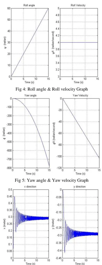
Fig 4: Roll angle & Roll velocity Graph

Fig 5: Yaw angle & Yaw velocity Graph

Fig 6:OWR X &Y positionwrt time Graph

The robot is falling according to friction affect as see in Figure 5.1.2.,Figure 5.1.3 shows the change of heading angle ϕ leaning angle ψ and robot position X and Y . Figure 5.1.4 shows time derivative of generalized coordinates, and the generalized speeds,Figure 5.1.1 shows position of a contact point of the robot on X-Y Plane. In leaning motion, the reaction wheel within a one-wheel robot produce momentum large enough to stabilize the robot. The gravity torque is also cancel and the robot is in dynamic equilibrium. Both the rolling disk and the

(7)

one-3746

behavior has been analyzed.

In order to formulate the equations of motion of a single wheel robot, we use assumptions appeared in as follows:

1) L2=0, so the mass center of the reaction wheel is coincident with the mass of the driving mechanism.

2) α = 0,Observed that the motion of the mass m, is too small and can be neglected at the steady state.

3) L1 = 0, such the mass center of the reaction wheel is coincident with the mass center of the disk.

4) Refer to assumption 3, driving torque from the mass m, will be absent. Such we assume that there is a Fictitious driving torque, T applied to the disk.

5) The spinning rate of reaction wheel β is set to be constant. Because of the momentum of the reaction wheel is too large, it is difficult to change or control its speed.

6) θ is control directly by tilt motor and can be treat as new input, θ ̇

CONCLUSION

We have solved the nonlinear numerical equation utilizing Matlab and graphically simulated the dynamic conduct of the Reactobot for differential initial conditions. The robot moves in a round way while its incline point progressively diminishes. In view of recreation, we found that the property of Reactobot is like moving plate if its response wheel is not turning. In examination with moving plate, all the more wobbling is seen in Reactobot. This is a result of pendulum development of Reactobot about pitch pivot. With some beginning speed along move hub, and some incline heavenly attendant and no torque, kinetic energy of Reactobot increments and potential energy diminishes. This is because, kinetic energy of falling object increases and potential energy decreases due to gravity. Reactobot trajectory shows circular path while falling on ground. By pivoting reaction wheel, the robot can direct to where it plans to go. On the off chance that consistent negative torque is connected then it moves round way towards its privilege and if steady positive (inverse) torque is connected, then it moves inverse i.e. towards its left.

Non-linear dynamical equation of movement of wheel robot were determined utilizing Kane’s method and Simulink model of system was produced taking into account the nonlinear numerical mathematical equation simulation were completed to examine the nonlinear independent conduct of wheel robot.reproduction result demonstrates that the robot falls in bearing of tilt point, come about additionally demonstrated that the Kane’s is alternative method in modelling of one wheel robot

Future Work

Complete nonlinear dynamic model of Reactobot is ready and verified that it is accurate. Nonlinear model is derived considering roll, pitch and yaw effects. We designed linear controller to stabilize it for vertical equilibrium position. Developed linear controller can be applied on Reactobot to stabilize it. After stabilizing it can be moved forward by applying torque to drive motor. Configuration of nonlinear controller is very prescribed for future examination. That

way, oscillatory developments of the robot while adjusting can be disposed of, hence exact direction control and waypoint route can be executed.

Nomenclature

Roll axis Axis parallel to the motion of wheel robot in horizontal plane

Pitch axis Axis perpendicular to the motion of wheel robot in horizontal plane

Yaw axis Axis perpendicular to the motion of wheel robot in vertical plane.

ϕ Yaw angle or precession angle of one wheel

θ Lean angle of wheel

ψ Spin angle of wheel about its axis ϕ ̇ Angular velocity about yaw axis θ ̇ Angular velocity about roll axis ψ ̇ Angular velocity about pitch axis α Rotation angle of reaction wheel α ̇ Angular velocity of reaction wheel R Radius of one wheel robot. r Radius of reaction wheel

IR Moment of inertia of one wheel robot about X,Y,and Z direction

Ir Moment of inertia of the reaction wheel about x,y and z axis

M Mass of one wheel.

m Mass of internal pendulum with reaction wheel

ACKNOWLEDGMENT

I give my true and sincere gratitude to Prof.S.N.Kadamand Prof.DivyaM.V.Padmanabhanfor his dedication and encouragement. Their passion and broad knowledge in robotics nourished my growth. I would like to thank them for giving me his ideas to do this work as well as for his guidance, support and inspiration throughout the course. To sum up, I would like to thank my friend with whom I had with. Of course, I don't have words to describe the support I received from my parents, My Father Prakash R.Borkar and My Mother DeeplaxmiP.Borkar.

.

REFERENCES

[1] S. N. Kadam and B. Seth, “LQR controller of one wheel robot stabilized by reaction wheel principle,” 2nd International Conference on Instrumentation Control and Automation ,Badung, Indonesia, no. November, pp. 299-303, 2011.

[2] Muhammad, Sbuyamin “Dynamic modeling and analysis of a two wheeled inverted pendulum robot”, IEEE, 2011

[3] J. Biswas and S. Bhartendu, “Dynamic Stabilisation of a Reaction-Wheel Actuated Reaction-Wheel-Robot,” International Journal of Factory Automation, Robotics and Soft Computing,no. 4, pp. 135-140, 2008 [4] W-nukulwuthiopas, “Dynamic Modeling of one wheel robot by using