CONSUMPTION SMOOTHING AND PORTFOLIO REBALANCING:
THE EFFECTS OF ADJUSTMENT COSTS
Yosef Bonaparte
Russell Cooper
Guozhong Zhu
Working Paper 16957
http://www.nber.org/papers/w16957
NATIONAL BUREAU OF ECONOMIC RESEARCH
1050 Massachusetts Avenue
Cambridge, MA 02138
April 2011
We are grateful to the National Science Foundation for supporting this research. We thank the Federal
Reserve Bank of Dallas for hosting us during the final stages of this project. The views expressed herein
are those of the authors and do not necessarily reflect the views of the National Bureau of Economic
Research.
NBER working papers are circulated for discussion and comment purposes. They have not been
peer-reviewed or been subject to the review by the NBER Board of Directors that accompanies official
NBER publications.
Consumption Smoothing and Portfolio Rebalancing: The Effects of Adjustment Costs
Yosef Bonaparte, Russell Cooper, and Guozhong Zhu
NBER Working Paper No. 16957
April 2011
JEL No. E21,G11
ABSTRACT
This paper studies the dynamics of portfolio rebalancing and consumption smoothing in the presence
of non-convex portfolio adjustment costs. The goal is to understand a household's response to income
and return shocks. The model includes the choice of two assets: one riskless without adjustment costs
and a second risky asset with adjustment costs. With these multiple assets, a household can buffer
some income fluctuations through the asset without adjustment costs and engage in costly portfolio
rebalancing less frequently. We estimate both preference parameters and portfolio adjustment costs.
The estimates are used for evaluating consumption smoothing and portfolio adjustment in the face
of income and return shocks.
Yosef Bonaparte
Robert Day School of Economics and Finance
Claremont McKenna College
500 East Ninth Street
Claremont, CA 91711-6400
yosef.bonaparte@claremontmckenna.edu
Russell Cooper
Department of Economics
European University Institute
via della Piazzola, 43
Firenze, 50133
ITALY
and University of Texas
and also NBER
russellcoop@gmail.com
Guozhong Zhu
Guanghua School of Management
Peking University
Beijing, China
The Effects of Adjustment Costs
∗
Yosef Bonaparte
†and Russell Cooper
‡and Guozhong Zhu
§April 10, 2011
Abstract
This paper studies the dynamics of portfolio rebalancing and consumption smoothing in the presence of non-convex portfolio adjustment costs. The goal is to understand a household’s response to income and return shocks. The model includes the choice of two assets: one riskless without adjustment costs and a second risky asset with adjustment costs. With these multiple assets, a household can buffer some income fluctuations through the asset without adjustment costs and engage in costly portfolio rebalancing less frequently. We estimate both preference parameters and portfolio adjustment costs. The estimates are used for evaluating consumption smoothing and portfolio adjustment in the face of income and return shocks.
1
Introduction
This research studies household saving and portfolio choice in the presence of non-convex portfolio adjustment costs. We ask: how do households respond to income and return shocks when portfolio adjustment is costly? The household optimization problem we study has two assets: one riskless without adjustment costs and a second risky asset with adjustment costs. This allows us to look at consumption smoothing and portfolio rebalancing separately. That is, the household could rebalance its portfolio, holding consumption fixed, or adjust consumption through a wide variety of asset trades. The costs of asset trading along with the preference parameters have not been estimated in a setting with multiple assets. These parameters are important for understanding the response of households to shocks to income and asset returns.
∗We are grateful to the National Science Foundation for supporting this research. We thank the Federal Reserve Bank of
Dallas for hosting us during the final stages of this project.
†Robert Day School of Economics and Finance, Claremont McKenna College, ybonaparte@cmc.edu
‡Department of Economics, European University Institute and Department of Economics, University of Texas at Austin and
NBER, russellcoop@gmail.com
1 INTRODUCTION
We consider the implications of an opportunity cost of asset trading and model it as a fraction of (stochastic) labor income. To match observed inaction of stock holdings, trading costs have a non-convex component. We estimate the opportunity cost of trading stocks, along with two other key parameters – the coefficient of relative risk aversion and the rate of time preference – via simulated method of moments.
Our study of how return shocks impact consumption is closely related to the estimation of inter-temporal elasticity of substitution (EIS). Traditionally EIS estimation is based on an Euler equation approach. Results from early studies, such as Hall (1988), conclude that the response of aggregate consumption to interest rate movements is near zero. More recently, Vissing-Jorgensen (2002), following Mankiw and Zeldes (1991), shows that it is imperative to distinguish between stockholders and non-stockholders in the estimation, because the Euler equation that links consumption growth to stock returns holds only for stockholders. However, in the presence of non-convex adjustment costs, as in our model, the standard Euler equation does not hold even for stockholders.
In terms of responses to income shocks, our model has the distinctive features of the buffer-stock saving model, as in Deaton (1991), Carroll (1992), Carroll (1997) and others. Households are impatient and accumulate wealth out of pre-cautionary motives. Consumption changes in response to income shocks, but is less volatile than income; while liquid wealth exhibits high volatility. However, in the traditional buffer-stock saving model, there exists only one asset – a risk-free bond. This makes it impossible for the traditional model to study the impact of income shocks on consumption smoothing and asset rebalancing jointly. The extension to multiple-asset model turns out to be difficult, as demonstrated in Heaton and Lucas (1997), because the return to risky asset is so high that the calibrated model generates near-zero bond holdings.
The portfolio choice literature offers extensive discussions on how labor income risks affect asset allocation. Empirical studies generally find that labor income risk reduces the share of risky assets in households’ financial wealth, as in, for example, Guiso, Jappelli, and Terlizzese (1996) and Angerer and Lam (2009). Theoretical studies by Koo (1995) and Heaton and Lucas (1997) find that investors hold most of their financial wealth in stocks, despite its riskiness. Koo (1995) and Elmendorf and Kimball (2000) show that an increase in the variance of permanent income shocks leads to a reduction in both the optimal portfolio allocation to stocks and the consumption-labor income ratio.
Simulation of the estimated model produces a number of interesting results. We do generate a positive demand for bonds. In an otherwise similar model without a non-convex opportunity cost of stock trading, Heaton and Lucas (1997) find it extremely difficult to explain the observed bond holdings in the data. Households hold bonds for two purposes, both are related to the infrequent adjustment of stock holdings due to adjustment costs. First, when households refrain from stock adjustment, bonds are used to smooth consumption. Secondly, when households make large scale changes to their stock account, bond holdings are adjusted to complement the stock adjustment. For example, after periods of inaction in adjusting its stock account, a household may find it optimal to reduce its stock holdings. In this case the household typically increases bonds on a large scale.
Buffer stock behavior is evident in our multiple asset model. The estimated discount factor is well below 0.80, so households hold financial assets for consumption smoothing purposes. The median wealth-income ratio is 2.14 in the model, which is the buffer stock for a typical household in the estimated model. Both stocks and bonds are used to buffer against income shocks. For small income shocks, a household will respond with variations in bond holdings, without incurring a costly stock adjustment. But, for large enough income shocks, stock holdings and bond holdings are jointly adjusted. Generally speaking, income shocks generate a negative co-movement between stock and bond holdings, for which we find empirical support.
We match the response of consumption growth rate to return shocks from the model to that in the data well. The response rate is 0.223 in our baseline model. The effects of return shocks on asset holdings are evident. At the household level, due to inaction in stock account, the correlation between bond and stock holdings is slightly negative. At the aggregate level, however, bond and stock holdings are clearly positively correlated. That is, a positive return shock increases both stock and bond holdings, and vice versa. Much of the impact of return shocks is absorbed by changes in asset holdings rather than consumption.
2
Model
We study the intertemporal consumption and portfolio choice of a household.1 The household’s portfolio consists of two assets. The first is an asset which is riskless and has a relatively low trading costs, such as money and bonds. We set this trading cost to zero. The second asset is stocks which have a higher return on average, are riskier and more costly to trade. Throughout we refer to the first asset as bonds and the second as stocks.
A household faces both income risk and variations in the return on stocks. Thus the household has a desire to both smooth consumption and adjust its portfolio in response to shocks.
The key aspect of the model comes from the costs of adjusting the household’s portfolio. If we assume that trades in bond are costless, then the agent can smooth consumption through this asset. But in some states, the agents will choose to adjust its holdings of stocks as well. This will generally lead to both portfolio adjustment as well as a change in the household consumption.
We look at an infinite horizon stochastic optimization problem.2 Letv(y, A−1, R−1) be the value of the
household’s problem. The state vector includes current household income y, the existing portfolio of A−1
and the return vector from the previous periodR−1. HereA−1= (Ab−1, As−1) is the vector of asset holdings
from the previous period, where Ab
−1 andAs−1 are the holdings of bond and stock respectively. The return
vector forR−1= (R−b1, R−s1) provides information about returns over the next period. Total financial wealth
equalsP
i=b,sR i
−1Ai−1.
1The model extends the household optimization problem studied in Bonaparte and Cooper (2010) by considering multiple
assets.
2To the extent that portfolio shares and asset market participation have life-cycle patterns, a life-cycle considerations may
2 MODEL
The value of the household’s problem is given by the maximum over the options of adjusting,va(y, A
−1, R−1),
or not,vn(y, A
−1, R−1), which is
v(y, A−1, R−1) = max{va(y, A−1, R−1), vn(y, A−1, R−1)} (1)
for all (y, A−1, R−1). Here adjustment refers to trading of stocks since trading of bonds is not costly.
If the household opts to adjust its stock account, the valueva(y, A−1, R−1) is given by
va(y, A−1R−1) = max
Ab≥Ab,As≥0u(c) +βER,y 0|R
−1,yv(y
0, A, R). (2)
The consumption level is given by
c= X
i=b,s
R−i1Ai−1+y×ψ− X
i=b,s
Ai−C(s−1, s). (3)
HereAiis the purchase of shares of asseti.
There are two costs of adjustment in this problem. The first, represented by the functionC(·), captures the direct cost of portfolio adjustment through payments to an intermediary. The second cost of adjustment, parameterized byψin (3), is meant to capture the total time cost of making an optimal choice about stock holdings. This cost occurs whenever a household make additions or reductions to stock accounts.3
If there is no adjustment of stock holdings, the value of the problem is:
vn(y, A−1, R−1) = max Ab≥Abu(c) +βER,y 0|R −1,yv(y 0, A, R). (4) where c=R1−1A−b1+y−Ab. (5) A= (Ab, As−1×Rs−1) (6)
When there is no adjustment of the risky asset, the household optimally adjusts its bond holdings. This is seen in (5), where consumption depends on the interest earnings on bonds as well as the purchases of bonds. The evolution of shares reflects the adjustment of bonds as well as no adjustment in stock holdings. Since we assume that dividends on stocks are reinvested without the payment of any adjustment cost, the transition forAis given in (6).
Notice that the choice of next period’s bond holdings is bounded below byAbwhile the holdings of stocks must be non-negative.4 IfAb <0, the household is able to borrow. We allow for borrowing in the model and discuss the estimation ofAb below.
3Thus, in contrast to the related literature on rational inattention, eg Abel, Eberly, and Panageas (2007) and Alvarez, Guiso,
and Lippi (2010), we study costs of trading rather than costs of becoming informed about the current state.
This problem includes both consumption smoothing and portfolio adjustment. It allows the household to partially smooth consumption through adjustment in their holdings of bonds. In addition, households can adjust their portfolio composition at a cost. We return to a discussion of the properties of these policy functions after estimating our model.
3
Parameterization and Estimation
This section discusses the parameterization of our problem. This includes the processes we use for income and returns to form the conditional expectations underlying the value functions in (1). We then discuss our estimates of key parameters.
3.1
Exogenous Processes and Financial Trading Costs
The Appendix provides a detailed discussion of the data used in our study. We take from the data the stochastic processes for income and returns as well as the moments used for our estimation. In addition, we estimate direct trading costs for stocks.
Income and Returns The income process for stockholders is estimated directly from the Panel Study of Income Dynamics (PSID). The persistence of income shocks is estimated at 0.842 with a standard deviation of the innovation to an AR(1) process of 0.29. We estimate the income process for stockholders because our model abstracts from stock market participation and every household is a stockholder.
The stock return comes from Shiller(http://www.econ.yale.edu/~shiller/data.htm). This return in-cludes both dividends and capital gains. The estimated serial correlation of annual returns is not significantly different from zero. We use two return states,−9.17% and 21.83%, with equal probabilites to approximate the stock return process. This implies an average annual return of 6.33% with a standard deviation of 15.5%. The non-stochastic return on bonds was set at 1.02. We discuss below the implications of allowing stochastic bond returns.
Trading Costs We allow the direct costs of trading stocks to vary depending on whether stocks are bought or sold:
Cb(As−1, As)) =ν0b+ν1b(As−As−1) +ν2b(As−As−1)2 (7) if the household buys stock so thatAs> As
−1. If instead the household sells stock, then
Cs(As−1, As)) =ν0s+ν1s(A−s1−As) +ν2s(As−As−1)2. (8) We take the estimates for these parameters from Bonaparte and Cooper (2010) who use monthly house-hold account data to estimate these transactions costs for the buying and selling of common stocks. Their estimates are summarized in Table 1. As noted by Bonaparte and Cooper (2010), only the fixed costs of
3.2 Estimation 3 PARAMETERIZATION AND ESTIMATION
trade are economically significant. Moreover, as these costs were estimated from the 1991-96 time period which preceded the PSID data, the actual fixed costs of traders may be less than that estimated here.
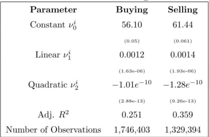
Table 1: Estimated Trading Costs Parameter Buying Selling Constant νi 0 56.10 61.44 (0.05) (0.061) Linearνi 1 0.0012 0.0014 (1.63e-06) (1.93e-06) Quadraticν2i −1.01e−10 −1.28e−10 (2.88e-13) (9.26e-13) Adj. R2 0.251 0.359 Number of Observations 1,746,403 1,329,394
3.2
Estimation
We estimate the preference parameters, (γ, β), along with the opportunity cost of stock adjustment, ψ, using simulated method of moments. We also use the estimates of trading costs from Table 1 as well as the stochastic processes for income and returns in this estimation. Finally, we discuss the procedure used to determine the borrowing limit,Ab.
3.2.1 Moments
We match four moments. The data appendix provides detailed information about the sources and calculation of these moments. These moments are for stockholders only which is consistent with our model.
The first moment is the adjustment rate for shareholders of 47% biannually. This moment is particularly informative about the opportunity cost of stock trading, one of the key elements in our model. We calculate it from five waves of the PSID survey, 1999-2007. The survey asked stockholders whether they bought or sold any non-IRA stocks since the previous interview. Within our sample, the percentage of stockholders that had positive answers ranged between 53% and 68% over the sample. This represents the gross adjustment rate. For these gross-adjustors, PSID further asked whether they put money into stocks, or took money out of them, or put about as much in as they took out. About 16.2% of the gross-adjustors reportedly put about as much in as they took out. On net, 47% of the stockholders either increased or decreased stock holdings, annually from 1999-2007. This net adjustment is consistent with the definition of stock adjustment in our model. In contrast, the gross adjustment includes rebalance between different stocks which is not considered in our model.5
It should be noted that the 47% biannual adjustment rate is not convertible into a 23.5% annual adjust-ment rate, unless totally different households undertake stock adjustadjust-ment in the two years. It might be, for example, that the same set of households adjust in both years, implying that the annual adjustment rate from PSID should also be 47%. We take this time aggregation into account in our estimation.
Bonaparte and Cooper (2010) calculate an adjustment rate of 71% from the Survey of Consumer Finance (SCF). The survey asks stockholders who own a brokerage account how many times they bought or sold stock over the past year. In Bonaparte and Cooper (2010), a stockholder is said to make stock adjustment if she bought/sold stocks at least once. The 71% annual gross adjustment rate is significantly higher than the 47% biannual gross adjustment rate in PSID. Notice that the SCF adjustment rate is for stockholders that own brokerage accounts, while the PSID adjustment is for all non-IRA stock holders. A higher adjustment rate in the SCF implies that stock holders that own brokerage accounts are more active traders.
The second moment is the portfolio composition of shareholders. We interpret bonds as the sum of deposits in transaction account and CDs, directly held bonds and saving bonds in the SCF. The data counterpart of stocks in the model is the amount invested in stocks (directly and indirectly) reported by SCF stock holders.
The fraction of stocks relative to the sum of stocks and bonds is 69%. This moment contains information on households’ degree of risk aversion (γ) and the opportunity cost of stock trading (ψ). The existing literature has found that a large coefficient of relative risk aversion is required in order to induce households to hold bonds due to the equity premium. We show that a smallerγcoupled with a modest portfolio adjustment cost,ψ near unity andC(·) small, induces sizable bond holdings, bringing the portfolio composition in the model closer to that in the data.
For the third moment, we follow the literature on intertemporal consumption and study the response of consumption growth to interest rate movements. This moment, termed the “EIS”, is computed from the consumption of shareholders, as in Vissing-Jorgensen (2002), with a point estimate of 0.2984.
The fourth moment is the median wealth to income ratio and is 2.127 in the data. This moment is important for estimating the discount factorβand relative risk aversionγ.6. Intuitively a highβis associated
with a high wealth-income ratio because households value future consumption. Similarly a highγ leads to high buffer-stock saving, hence a high wealth-income ratio.
To estimate the parameters, we solve
Γ =min(γ,β,ψ)(Ms−Md)0W(Ms−Md). (9)
Here Md are the moments from the data and Ms are the simulated values of those moments for a given set of parameters, (γ, β, ψ). The weighting matrix,W, is the inverse of a matrix with the variances of the moments along the diagonal. Since our moments come from different data sources, we are unable to calculate covariances directly.
3.2 Estimation 3 PARAMETERIZATION AND ESTIMATION
The simulated moments are obtained by solving the household’s dynamic optimization problem through value function iteration. The solution method is described in the Appendix. Through simulation, a panel with 500 households and 800 time periods is created. The simulated moments are calculated from this panel in exactly the same manner as they are calculated in the actual data. In particular, the adjustment rate is calculated bi-annually in the simulated data as it is in the PSID.
Throughout this analysis, we focus on financial wealth, ignoring housing and other durables. Further, the portfolio share relates to financial assets alone. The consumption measure includes the service flow from housing. This is consistent with a model in which housing is rented by households who hold a portfolio of financial assets. This is also the outcome of a model in which the housing stock is held by households and is costlessly adjusted.
3.2.2 Results
The results are presented in Table 2. The first row in the table summarizes the data moments. The second row contains our results.
These results are for the case ofAb= 0 so that households are unable to borrow on their bond accounts. The restriction ofAb = 0 comes from estimating this lower bound along with the other parameters of the model. In the end, the best fit was with the tightest borrowing constraint ofAb= 0.
The baseline results are indicated by the “Est. Model” row. The moments are presented first followed by the parameter estimates. The standard errors for the baseline estimates are indicated as well. These are computed from the matrix of numerical derivatives of the moments with respect to the parameters combined with the variance matrix used as weights following Adda and Cooper (2003). Table 7 of the Appendix shows the elasticities of the moments with respect to the parameters which is an input into the computation of the standard errors. This table is also informative about identification as it indicates which moments are particularly sensitive to variations in each of the parameters.
The simulated moments are all reasonably close to the actual data moments. The adjustment rate and median wealth-income ratio are met almost exactly. In contrast to Heaton and Lucas (1997), our model generates positive demand for low return riskless bonds. The share of bonds in total financial wealth is about 26%. The major reason for the increased demand for bonds is the opportunity cost of stock trading.
The parameter estimates indicate that a low discount factor of 0.7048 is necessary to match these mo-ments. As noted earlier, the median ratio of wealth to income is particularly sensitive to the discount factor. The role of stochastic labor income is important here. As in Deaton (1991) and Carroll (1992), with such a low discount factor, neither stocks nor bonds would be demanded in the absence of uninsurable income risk. The estimate ofγindicates a curvature of about 6.4, which is not the same as the inverse of the estimated EIS from the data. In the model with adjustment costs, there is no direct link between the inverse of the EIS and preference parameters. As we discuss below, the response of aggregate consumption growth to variations in the return depend on both the extensive (the choice of adjusting or not) and the intensive margins.
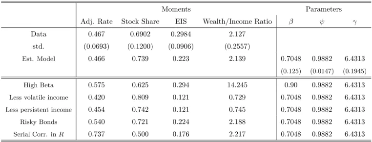
Table 2: Estimation Results and Robustness
Moments Parameters
Adj. Rate Stock Share EIS Wealth/Income Ratio β ψ γ
Data 0.467 0.6902 0.2984 2.127
std. (0.0693) (0.1200) (0.0906) (0.2557)
Est. Model 0.466 0.739 0.223 2.139 0.7048 0.9882 6.4313
(0.125) (0.0147) (0.1945)
High Beta 0.575 0.625 0.294 14.245 0.90 0.9882 6.4313
Less volatile income 0.420 0.809 0.121 0.729 0.7048 0.9882 6.4313
Less persistent income 0.454 0.742 0.121 0.745 0.7048 0.9882 6.4313
Risky Bonds 0.540 0.721 0.224 2.188 0.7048 0.9882 6.4313
Serial Corr. inR 0.737 0.500 0.176 2.217 0.7048 0.9882 6.4313
The point estimate of the adjustment costs is 1−ψ= 0.012. With average income of about $72,000 in the data used to estimate the trading costs reported in Table 1, this part of the adjustment cost is about $850. Combined with the estimated fixed cost of financial trades, the total fixed cost is around $905.
The fit of the model, Γ, is 0.8675. We have three parameters and four moments. With one degree of freedom, the p-value is 0.352 and thus Γ is not significantly different from zero at a 5% level. The model is not statistically rejected. But, keep in mind that the weighting matrix assumes that covariances are all zero.
3.2.3 Robustness
The bottom rows of Table 2 show the results from some additional experiments. These are intended to explore the robustness of our results. There is no additional estimation involved here, just simulations with different parameterizations.
In the first experiment, β is increased to a more traditional level of 0.90. Given how low our estimate is relative to other studies, it is important to know why such a low value is needed to match our moments. As shown in the table, the higher value ofβ generates a wealth/income ratio much higher than in the data. While the other moments are also affected by this largeβ, it is clear that matching the data wealth/income ratio requires more discounting than usual.
The procedure used to generate our approximation of the household income process is outlined in the Appendix. The process we use is more persistent and more volatile than in some other studies. For example, Heaton and Lucas (1997) assume a serial correlation of 0.53 and standard deviation of income innovations equal to 0.24.
Our second and third experiments study how the simulated moments change with alternative income processes. The “Less volatile income” case replaces the income process estimated in the PSID with one in
4 RESPONDING TO SHOCKS
which the innovation to the income process is 0.20 rather than 0.29 in the baseline. The portfolio choice literature has both empirical evidence and theoretical argument that less risky labor income should be associated with less saving and more investment in risky assets. This is also found in our model – from the baseline case, wealth-income ratio decreases from 2.139 to 0.729, and stock share rises from 0.739 to 0.809. So while we can still generate bond holdings, it is clear that this share is sensitive to the volatility of the income process due to the presence of portfolio adjustment costs.
The “Less persistent income” case replaces the income process estimated in the PSID with one in which the persistence of the innovation to the income process is 0.60 rather than 0.842 in the baseline. This has very similar effects as the experiment with less volatile income innovations. This is partly by construction since the reduction in the serial correlation induces less volatile income, given the standard deviation of the income innovations. Still, in this case the stock share remains close to that in the estimated model as does the adjustment rate. But the wealth income ratio is quite low.
The “Risky Bonds” case allows the return on bonds to be stochastic. The bond process is estimated from Shiller data for the sample period of 1947 to 2007. The mean return is 2%, the standard deviation of the innovation is 0.0266 and the serial correlation is 0.57. This contrasts with the zero serial correlation of stocks. The moments change very little in response to adding these shocks to the model.7
The final experiment allows households to believethat return shocks are positively serially correlated. As discussed in Bonaparte and Cooper (2010), the higher serial correlation can be interpreted as household’s placing excessive weight on current realizations of returns, a form of overconfidence. To be clear, in this case, we modify household beliefs so that the perceived serial correlation in returns is 0.30, though actual returns that underlie the simulated data are iid.8
As indicated in the “Serial Corr.” row, households are more prone to adjust their portfolios since the gains to adjusting are higher the more persistent are the shocks. With this higher perceived serial correlation and hence higher variability in returns, the stock share is lower.
4
Responding to Shocks
Given these estimates, we turn to a main point of our study: how do households respond to income and return shocks? This is a traditional question of the consumption and portfolio choice literature. Our answer differs because of the presence of portfolio adjustment costs.
We first present and discuss the policy functions of our estimated model. We then turn to simulation results to display the properties of these policy functions.
0
0.5
1
1.5
2
0
0.5
1
1.5
2
policy functions (low income)
bond
stock
0
1
2
3
4
0
1
2
3
4
policy functions (median income)
bond
stock
0
2
4
6
0
2
4
6
policy functions (high income)
stockholding
bond
stock
Figure 1: Policy functions.
This figure shows the policy functions for three different income states. Current stock holdings (including current returns) are shown along the horizontal axis. Future stock and bond holdings are indicated along the vertical axis.
4.1 Policy Functions 4 RESPONDING TO SHOCKS
4.1
Policy Functions
Figure 1 shows the decision rules (policy functions) for future stock and bond holdings as a function of current stock holdings. Here, the measure of current stock holdings includes the realized return on stocks: in the notation of the model this isAs
−1Rs−1. The decision rules are shown for three different realizations of
income. Current period’s bond holdings are fixed at the average of the simulated panel (about 26% of mean income) and the return state is at its mean of 6.33%.
The decision rules are plotted together with the 45 degree line. Given the inaction in stock adjustment created by the non-convex adjustment costs, future stock holdings can be the same as current stock holding, indicated by decision rules which coincide with the 45 degree line.9
The upper panel is for a household whose income realization is at low level, one standard deviation below the mean. The middle panel is for a household whose income realization is at the mean. The lower panel is for a household whose realized income is one standard deviation above the mean.
As indicated in these policy functions, there is a sizable inaction region for stock adjustment for all three income states. It is only in the tails of the current stock holdings that adjustment in this margin occurs. Over these regions of inaction, in which the stock return is re-invested automatically, bond holdings are a decreasing function of the stock holdings. As the value of the stock account increases, households will consume at a higher level. This is financed by lower bond holdings. Thus bond holdings are valuable even though the bond return is much lower than the stock return.
The size of the inaction region also depends on the income shock: in the low income state, the inaction range is narrower and the critical values of current stockholdings defining the inaction region are lower. This is partly reflecting the interaction of adjustment costs with income: the opportunity cost of trading is lower when income is low. Further, the gains to adjustment are larger in the low income state since households want to smooth consumption by drawing upon their stock holdings.
When adjustment of the stock account does occur, the bond holdings move in the opposite direction. So, for example, high income households with very large stock holdings will reduce their stock accounts in order to finance higher consumption. They also increase bond holdings so that consumption can be smoothed out of bonds in the future inaction periods.
As indicated in Figure 1, the bond policy function is very non-linear even though the adjustment costs only apply to stocks. Of course, once the adjustment cost is paid for stocks, then the choice of bond holdings is quite different from the states of no adjustment in stocks.10
7Estimating the model with this additional state variable is very time consuming. Hence the baseline estimation and all of
the following exercises assume a constant bond return.
8We also re-estimated the model with these beliefs and could not improve upon the baseline model.
9For these figures, the current stock holding includes return. Hence inaction is represented when the policy function coincides
with the 45 degree line.
10This type of spillover is found in other optimization problems in which a non-convex adjustment cost applies to only a
subset of the choice. For example, in a dynamic capital adjustment problem with no adjustment costs of labor, the nonlinearity in the capital decision rule will induce a nonlinearity in the labor decision rule.
4.2
Simulation Results
To illustrate the choice problem of agents, we study some simulation results. This enables us to see the response to households to income and return shocks. These responses indicate how households use their portfolios to smooth consumption as well as portfolio rebalancing in response to income and return variations. The figures, which summarize the simulations, show stock and bond holdings as control variables over time. Further, the stock holdings series has diamonds to indicate periods of inaction.
4.2.1 Response to income shocks
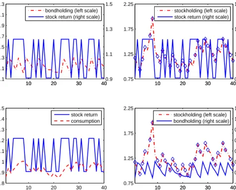
Given the presence of the fixed adjustment costs, the response to income shocks is nonlinear. Accordingly we distinguish the response of the household to relatively small income shocks, as shown in Figure 2, from the response to larger income shocks, as shown in Figure 3.
5 10 15 20 25 30 0 0.16 0.32 0.48 0.64 0.8 5 10 15 20 25 30 1 1.16 1.32 1.48 1.64 1.8 5 10 15 20 25 30 0.8 0.9 1 1.1 1.2 1.3 periods 5 10 15 20 25 30 1 1.16 1.32 1.48 1.64 1.8 periods 5 10 15 20 25 300.8 0.9 1 1.1 1.2 1.3 bondholding (left scale) income (right scale)
5 10 15 20 25 300.8 0.9 1 1.1 1.2 1.3 stockholding (left scale) income (right scale)
income consumption 5 10 15 20 25 300 0.16 0.32 0.48 0.64 0.8 stockholding (left scale) bondholding (right scale)
The figure plots the dynamics of stock holdings, bond holdings and consumption in response to a small income shock. The stock return is fixed at the average level (6.33% per year). Diamonds mark inaction of stock account.
Figure 2: Small income shock.
As indicated in the top left panel of Figure 2, a household’s bond holdings increase with an income shock. From the bottom left panel, there is also an increase in consumption at the time of the shock. Since the income shock is relatively small, stock holdings do not instantly change, as indicated by the top right panel. Instead, stock holdings build through the reinvestment of dividends without any adjustment (as indicated
4.2 Simulation Results 4 RESPONDING TO SHOCKS
by the diamond). After a few periods, the stock account has grown enough to warrant an adjustment. At the time of adjustment (periods 5, 10, etc.), the stock account falls and the bond account grows, as shown in the bottom right panel.
Thus these figures combine two effects. The first is the response to the temporary income shock. The second is the ongoing interaction between the stock and bond accounts. Due to the fixed cost, there is a natural dynamic of infrequent adjustment from the stock account to the bond account (portfolio rebalancing) along with the financing of consumption from the bond account (consumption smoothing). These dynamics are akin to those found in the literature on money demand associated with Baumol and Tobin.
The response to a larger income shock is somewhat different. Looking at the top right panel of Figure 3, the larger income shock induces an immediate response of stock adjustment. The increase in the stock account implies that the bond account does not increase proportionately as much with the larger income shock, than it did with the smaller income shock. This is seen by the top left panel. Consumption responds to the income shock as before. Once the response to the income shock is over, the usual dynamic of portfolio rebalancing occurs again, as shown in the bottom right panel.
5 10 15 20 25 30 0 0.4 0.8 1.2 1.6 2 2.4 5 10 15 20 25 300.6 1.1 1.6 2.1 2.6 3.1 bondholding (left scale) income (right scale)
5 10 15 20 25 30 0.8 1.8 2.8 3.8 4.8 5 10 15 20 25 300.6 1.1 1.6 2.1 2.6 3.1 stockholding (left scale) income (right scale)
5 10 15 20 25 30 0.5 1 1.5 2 2.5 3 periods income consumption 5 10 15 20 25 30 0.8 1.8 2.8 3.8 4.8 periods 5 10 15 20 25 300 0.4 0.8 1.2 1.6 2 2.4 stockholding (left scale) bondholding (right scale)
The figure plots the dynamics of stock holdings, bond holdings and consumption in response to a large income shock. The stock return is fixed at the average level (6.33% per year). Diamonds mark inaction of stock account.
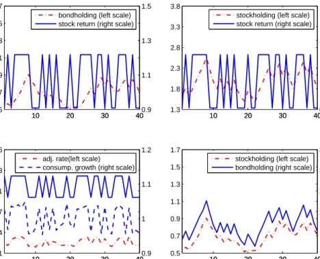
4.2.2 Response to Return Shocks
We now study the response of households to return shocks. This is illustrated in Figure 4. For this simulation, income is held at its mean and initial stock holdings and bond holdings are both the averages of the simulated path of 500 households for 800 periods.
Households generally increase (decrease) their stock holdings, bond holdings and consumption in response to a positive (negative) shock to stock return. Nevertheless, the adjustment in asset holdings is of a very large scale, while consumption adjustment is relatively small. This response shows both consumption smoothing and portfolio rebalancing at work.
However, the co-movement of return with either stock or bond holdings is complex. The upper-right panel shows that stock adjustment is very infrequent. During the inaction, bond account is adjusted, either in the same direction as return or the opposite. For example, suppose stock holdings are high and there is a high stock return. If a household decides not do adjust its stock account, it is optimal for the household to reduce bond holdings to finance consumption. In this case, bond holdings and stock return move in the opposite direction. Due to this kind of portfolio rebalancing, there is a negative correlation of -0.103 between stock and bond holdings at the individual level.
10 20 30 40 −0.1 0.1 0.3 0.5 0.7 0.9 1.1 1.3 10 20 30 40 0.75 1.25 1.75 2.25 10 20 30 40 0.8 0.9 1 1.1 1.2 1.3 1.4 1.5 periods 10 20 30 40 0.75 1.25 1.75 2.25 periods 10 20 30 400.9 1.1 1.3 1.5 bondholding (left scale) stock return (right scale)
10 20 30 400.9
1.1 1.3 1.5 stockholding (left scale) stock return (right scale)
stock return consumption 10 20 30 40−0.1 0.1 0.3 0.5 0.7 0.9 1.1 1.3 stockholding (left scale) bondholding (right scale)
The figure plots the dynamics of individual stock holdings, bond holdings and consumption in response to shocks to stock return. Income is fixed at its mean level.
Figure 4: Return shocks and individual decisions
4.2 Simulation Results 4 RESPONDING TO SHOCKS
at the bottom right panel, at the aggregate level the correlation between stock and bond holdings is clearly positive. In fact, it equals 0.94 in contrast to the negative correlation found at the individual level. The aggregate correlation is a different sign since the aggregation smooths over the lumpy portfolio adjustment at the individual level.11
Second, as seen in the bottom left panel, the correlation between consumption growth and the stock return (also shown in that panel) is evident as well. Both the correlation of the adjustment rate with consumption growth and the correlation of the adjustment rate with the stock return are positive. The comovement of consumption growth and stock returns, amplified by the adjustment decision, underlies the regression results used as a moment in Table 2.
10 20 30 40 0.5 0.7 0.9 1.1 1.3 1.5 1.7 10 20 30 400.9 1.1 1.3 1.5 bondholding (left scale) stock return (right scale)
10 20 30 40 1.3 1.8 2.3 2.8 3.3 3.8 10 20 30 400.9 1.1 1.3 1.5 stockholding (left scale) stock return (right scale)
10 20 30 40 0.1 0.4 0.7 1 1.3 1.6 periods 10 20 30 400.9 1 1.1 1.2 adj. rate(left scale)
consump. growth (right scale)
10 20 30 40 0.5 0.7 0.9 1.1 1.3 1.5 1.7 periods 10 20 30 401.3 1.8 2.3 2.8 3.3 3.8 stockholding (left scale) bondholding (right scale)
The figure plots the dynamics of aggregate stock holdings, bond holdings and consumption in response to shocks to stock return. Income is fixed at its mean level.
Figure 5: Return shocks and aggregate decisions
4.2.3 Regression Results
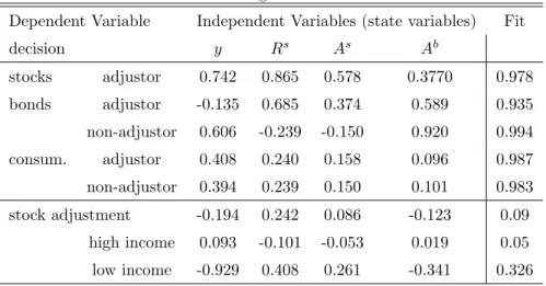
For further evidence on the structure of household decision rules, we study the state-dependence of bond holdings, stock holdings and consumption as well as the adjustment decision through a regression structure. Although the regressions are only coarse approximations, they are illustrative of the forces at work. Our
11A similar result is reported for the correlation between hours and employment at the plant-level and in aggregate by Cooper,
results are shown in Table 3.
The first five rows report the regressions of decisions regarding stock holdings, bond holdings and con-sumption on current state variables: income, stock return, stock holdings and bond holdings. These regres-sions are run at the household level from the same simulated panel used to calculate our moments.
Each regression yields a very high R-squared, indicating highly linear decision rules. These are intensive margin decisions because we split households into adjustors and non-adjustors. It is noteworthy that these decisions are so linear though there is a nonlinear dimension to the problem associated with the adjustment decision.
Adjustors and non-adjustors have quite different decision rules. Bond holdings of adjustors is negatively correlated with income due to the substitution between stocks and bonds as shown in the impulse response figures – when stock adjustment occurs, it is accommodated by bond adjustment in the opposite direction. For non-adjustors, higher current income leads to higher future bond holdings in order to smooth consump-tion. However, stock return and current stock holdings are negatively correlated with future bond holdings. Due to wealth effect, high stock return and current stock holdings induces more consumption which is fi-nanced by reduced bond holdings. The marginal effect of state variables on consumption decisions are about the same for adjustors and non-adjustors, implying good consumption smoothing.
The last three rows report linear regressions of the state-dependent adjustment decision. The first line shows the results of a pooled regression indicating that adjustment is reduced by an income shock and is increased by a return shock. This is consistent with the findings from the simulated data which highlighted the dependence of the inaction region on income. The adjustment rate is lower when bond holdings are higher since the bond holdings are adequate for buffering income shocks.
Given the discussion in Section 4.2.1, it is interesting to look for asymmetries in the decision rule. This is illustrated by splitting the sample into high income (above average) and low income (below average) states. The results are reported in the last two rows of the table. The results for the low income sub-sample have the same signs as those from the pooled data. An income shock reduces the likelihood of adjustment since the household uses that additional income to smooth consumption. This effect is quite strong. By a similar logic, in the low income state, if there is a return shock, then adjustment is more likely since the household can take funds from the stock account and use them for consumption smoothing.
For the high income sub-sample, the signs switch on all of the state variables, indicating the asymmetric response. Further, the responses are muted, compared to the low income sub-sample. When income is above average, the household is looking to smooth consumption by saving more. Thus an income shock makes the household more likely to adjust. But, in the high income state, the high return on the portfolio is not needed for consumption smoothing and thus the adjustment probability is lower. The same argument holds for the coefficients on the stock and bond accounts in the high and low income states.
4.2 Simulation Results 4 RESPONDING TO SHOCKS
Table 3: Regression Results
Dependent Variable Independent Variables (state variables) Fit
decision y Rs As Ab stocks adjustor 0.742 0.865 0.578 0.3770 0.978 bonds adjustor -0.135 0.685 0.374 0.589 0.935 non-adjustor 0.606 -0.239 -0.150 0.920 0.994 consum. adjustor 0.408 0.240 0.158 0.096 0.987 non-adjustor 0.394 0.239 0.150 0.101 0.983 stock adjustment -0.194 0.242 0.086 -0.123 0.09 high income 0.093 -0.101 -0.053 0.019 0.05 low income -0.929 0.408 0.261 -0.341 0.326
4.2.4 Substitution Between Stocks and Bonds – Data Evidence
One of the most notable phenomena in the simulation results is the substitution between stock and bond holdings, which is a direct result of the infrequent adjustment of the stock account due to non-convex adjustment costs.
Specifically, when the stock account is not adjusted, bond holdings is adjusted for consumption smoothing purposes. This typically results in a negative correlation between changes in stock holdings and bond holdings, because the stock return is positive on average and non-adjustment means an increase in the stock account. The negative correlation also arises when stock holdings are too high and adjustment takes place. In this case stock holdings are reduced, while bond holdings are replenished.
We look at PSID data and find evidence supporting this negative correlation. Since 1999, the PSID provides wealth supplements bi-annually. Thus we employ the panel structure of data on stock holdings, bond holdings and income to study their correlations. Data description and sample selection criteria are given in the appendix.
We pool data from different years and regress income, bond holdings and stock holdings on age, age-squared, education dummies and sex-of-head dummy. The residuals, denotedyi,t,Bi,t andSi,t respectively,
are income, bond holdings and stock holdings with demographics controlled for, and thus are comparable with simulated data. Define ∆Bi,t=Bi,t-Bi,t−1, then ∆Bi,t is the change in bond holdings, which can be
obtained from PSID data. We also obtain ∆yi,tand ∆Si,t from the data, and calculate correlations between ∆yi,t, ∆Bi,t and ∆Si,t. The same correlations are also calculated from simulated data. Notice that t
represents two years because surveys take place every two years.
Table 4 reports the correlations both in the data and the model, together with bootstrapped standard errors. The correlation between changes in stock holdings and bond holdings is negative – -0.338 in the data and -0.467 in the model, both are statistically significant. The correlations between ∆ytand ∆St are
Table 4: Correlations data model ∆yt ∆Bt ∆St ∆yt ∆Bt ∆St ∆yt 1 1 ∆Bt -0.062 1 0.005 1 (0.036) (0.002) ∆St 0.117 -0.338 1 0.357 -0.467 1 (0.015) (0.072) (0.002) (0.003)
Correlation between income, bond holdings and stock holdings. ∆Yt, ∆Bt and ∆St are changes
in income, bond holdings and stock holdings respectively. In parenthesis are bootstrapped standard errors.
positive both in the data and model. Correlation between ∆ytand ∆Btis slightly negatively in the data, but slightly positive in the model. Overall, the correlations in the data are consistent with the argument that adjustment costs lead to the substitution between stock and bond holdings.
5
Conclusion
This study asked how households respond to income and return shocks when there are portfolio adjustment costs. We estimate the opportunity cost of stock trading, along with discount factor and curvature in preference via simulated method of moments.
We find that this response comes in two forms: portfolio rebalancing and consumption smoothing. The response is highly nonlinear. The stock account is adjusted in response to large income shocks while the bond account buffers consumption from smaller shocks. Our simulation results reveal a strong negative correlation between stock and bond holdings at the household level. When households refrain from adjusting stock accounts to avoid costs, their stock account is increased due to the re-invested dividend, but the bond account is run down to finance consumption. On the other hand, when stock adjustment occurs, the bond account is replenished. We find data evidence in PSID supporting such substitution.
Variation in stock returns leads to mild variation in consumption, but large-scale changes in both bond and stock holdings. Due to inaction in stock trading, household stock holdings and bond holdings exhibit slightly negative correlation when return shocks are present but income shocks are shut down. At the aggregate level, stock and bond holdings have a correlation close to unity. In summary, both consumption smoothing and portfolio rebalancing are evident in response to return shocks.
6 APPENDIX
6
Appendix
6.1
Data Appendix
Exogenous processes We calculate the stock return process from Robert Shiller’s online data ofS&P500 for the period 1947-2007. The return is defined as pt+1+dt
pt whereptisS&P500 index anddtis the dividend. The return is then deflated by the CPI. We run an AR(1) regression on stock return, and we find that the persistence is not statistically different from zero. So we represent stock return as an i.i.d. process. The mean and standard deviation of return are 6.33% and 15.5% in our sample period.
The income process is calculated from the Panel Study of Income Dynamics (PSID) for the period of 1968-1997. Income is defined as salary plus other source of labor income such as commission, overtime, labor part of business income, labor part of farm income and others. Totally there are 78 households who have complete income information during the 30 years and satisfy the following criteria (i) non-SOE sample12
(ii) full information on age, gender, marital status, and education attainment (iii) stockholders. The survey does not provide stock holdings information except in years 1984, 1989 and 1994 during the sample period. So we drop all the households that are not stockholders during the three waves of survey in order to meet criterion (iii).
We take two steps to calculate the size and persistence of income shocks.
1. Pool all the observations together, and regress income on age,age2, education attainment, gender and marital status.
2. Take the residuals from the above regression, and use the residuals to run the AR(1) process
yt=ρyt−1+t.
The persistence of income shock is estimated to beρ= 0.84224, and standard deviation of the innovation is
σ= 0.29027.
Data moments We calculate data moments from 3 sources: Survey of Consumer Finance (SCF), Panel Study of Income Dynamics (PSID), and the consumption data complied and used in Vissing-Jorgensen (2002). We use multiple sources for two reasons. First, it is impossible to calculate all the moments in a single data. Secondly, each data source has its own strength and drawbacks, so we choose the best combination possible.
We calculate two moments from the SCF: the median of stock share in total financial wealth, and median wealth-income ratio, using 7 waves of the SCF (1989, 1992, 1995, 1998, 2001, 2004 and 2007). In each wave, we first calculate the ratios at the household level, then calculate the median of the household level ratios. Although the SCF provides a weight for each household, we use an un-weighted median. This is because our sample includes stockholders only, while the SCF weights are meant to make the whole
Table 5: Moments from SCF
1989 1992 1995 1998 2001 2004 2007 average median Stocks share 0.479 0.571 0.691 0.782 0.786 0.749 0.773 0.690 median Wealth/income 1.942 2.020 1.843 2.042 2.099 2.369 2.573 2.127
Table 6: Stock adjustment rate from PSID gross adjustment rate net adjustment rate
1999-2001 68% 57%
2001-2003 53% 44%
2003-2005 53% 44%
2005-2007 56% 42%
average 58% 47%
sample, including non-stockholders, nationally representative. The SCF is known for its excellent quality of information on household’s asset-holdings. In addition, it provides detailed information on labor force participation, liabilities, and other social demographic characteristics such as age, education and gender. The survey also collects information on total family earnings and wealth. The actual number of respondents in the survey is approximately 4,300 where for each observation there are another five imputed observations. Stock holdings in the SCF are defined as the sum of directly and indirectly held stock market investment. We define bond hooldings as the sum of investment in transaction accounts, CDs, directly-held bonds and saving bonds. Total financial wealth is defined as the sum of stock investment and bond investment. Income reported in the SCF is the total income from wage and salaries before deduction for taxes. Table 5 reports the moments for various years and the average over the years.
We calculate the moment of stock adjustment rate from PSID, using the 1999-2007 sample period. Start-ing from 1999, PSID surveys are conducted bi-annually, each wave provides wealth supplements which include information on the respondents’ holdings of non-IRA stocks. The survey asks three questions regarding stock adjustment: (i) whether the respondent buy stock since last survey, (ii) whether sell stock since last survey, (iii) whether buy more, sell more, or put as much in as took out. We define “gross adjustment rate” as the percentage of households who answered positively to either question (i) or (ii). The gross adjustors include the subset of households who report “put as much in as take out”. This subset of households did rebalance among different stocks, but didn’t use stock for consumption smoothing purpose. We exclude these house-holds from gross adjustors, and define the remaining as net adjustors. The adjustment rate consistent with our model definition is “net adjustment rate” – the percentage of households who are net adjustors. Table 6 shows the gross adjustment rates and net adjustment rates for the four intervals in our sample.
The response rate of aggregate consumption to stock return is calculated from data used in Vissing-Jorgensen (2002). The data are semi-annual, so we convert the consumption growth rate and return into
6.2 Computation Appendix 6 APPENDIX
annual data by taking geometric means. As in Vissing-Jorgensen (2002), we run two-stage least square to obtain the response of consumption growth to stock return, using the growth rate of dividend as the instrument. Changes in family size are also controlled for.
Dynamics of income and asset-holdings in PSID We study the dynamics of income asset-holdings empirically based on the PSID 1999-2007. The sample includes households that (i) have complete income information during the sampling period (ii) are stockholders (iii) have valid information on education attain-ment, age of head and sex of head in 1991 (iv) are aged 48 or less in 1991 so that they do not retire during the sampling period (v) have valid information on bond holdings and stock holdings. Totally there are 298 households in the sample.
Besides housing wealth, the PSID has three types of wealth: (i) non-IRA stock (ii) money in checking or savings accounts, money market funds, certificates of deposit, government savings bonds, or treasury bills (checking and saving) (iii) other savings or assets, such as bond funds, cash value in a life insurance policy, a valuable collection for investment purposes, or rights in a trust or estate (bond and insurance). In addition, the wealth supplements provide information on debt that does not include home or vehicle loans, such as credit card charges, student loans, medical or legal bills, or on loans from relatives. We group wealth into two categories: stocks and bonds. Stocks are simply the non-IRA stocks. Bonds are defined as “checking and saving + bonds and insurance - debt”.
6.2
Computation Appendix
The state space of the dynamic optimization problem in our model is (y, A−1, R−1). Here y is income of the
current period, A−1 = (Ab1, As−1) is the vector of beginning-of-period asset holdings, andR−1 = (Rb1, Rs−1)
is the vector of bond return and stock return.
The income process is represented by a 5-state Markov chain. The i.i.d. stock return process is approx-imated by two return states,−9.17% and 21.83% with equal probability, implying a mean return of 6.33% and a standard deviation of 15.5%. The bond return is fixed in the baseline case, and is not kept track of in the programming problem. In the robustness check we allow the bond return to be risky and persistent, and approximate the process by a two-state Markov chain.
The dynamic programming problem has 3 discrete state variables and 2 continuous state variables (stock holdings and bond holdings). There are 2 control variables – a household needs to decides how much stock and bond to hold in the beginning of each period. This is a high-dimensional programming problem which is computationally intensive. Furthermore we need to solve the model many times to find parameter values that best match model moments with data moments. In order to solve the model with good precision within a reasonable amount of time, we take the following strategy.
First, we combine stock return and stock holdings into one state variable. This is feasible because the stock return is i.i.d. That is, the current stock return contains no information about next period’s return.
Therefore we can simply treat stock holdings after the realization of return as a state variable, rather than keep track of both stock return and stock holdings before the realization of return. Notice that stock holdings as a control variable refers to the holding before the realization of return. In simulation, we solve for stock holdings as a control variable, then multiply it with the return to make it a state variable for the next period. Second, we use a mixture of grid search and spline interpolation to execute value function iteration. Specifically, we define two grids for the Cartesian space of stock holdings and bond holdings. The first one is a coarse grid with 25 points for stock holdings and 20 points for bond holdings, denotedAs
coarse×Abcoarse.
The second one is a fine grid with 400×150 grid points, denotedAs
f ine×Abf ine. We start with an initial
guess of value functionv(D, As
f ine×Abf ine) whereD stands for the product of discrete state variables. Then
we take the following steps to update the value function.
1. On the coarse grid, compute the value of the sub-optimal decision of not adjusting stock holdings, denoted vn(D, As
coarse×Abcoarse). The value of the sub-optimal decision of always adjusting stock
holdings, denotedva(D, As
coarse×Abcoarse), is also computed.
2. Usevn(D, Ascoarse×Abcoarse) andva(D, Ascoarse×Abcoarse) to interpolate the values on fine grid, denoted vn(D, Asf ine×Abf ine) andva(D, Asf ine×Abf ine). Due to the high non-linearity of the value functions, we using spline interpolation.
3. Compute the updated value function asv(D, As
f ine×Abf ine) = max{vn(D, Asf ine×Abf ine), va(D, Asf ine× Ab
f ine)}.
After the value function converges, we compute policy functions on the fine space, and use these policy functions to simulate artificial data. In the simulation, we draw random shocks to income and returns of 500 households for 800 periods, so the dimension of simulated data is 500×800.
Third, we design both coarse grid and fine grid carefully. The upper-bounds of asset holdings grid are important. Very high upper-bounds reduce the efficiency of the program, because a large area of the grid near the upper-bounds are never reached in simulation. On the other hand, when the upper-bounds are too low, households’ optimal decision rules are distorted. After many experiments, we find that the upper-bounds of 40 times of mean income for stock holdings and 20 times of mean income for bond holdings are efficient and non-binding. In addition, we put more points near the lower-bounds of the asset holdings grid.
6.3
Parameter Sensitivity
Table 7 summarizes the elasticity of the moments (cols) to variations in the parameters (rows). This matrix is an input into the computation of the standard errors. It also is informative about identification as it indicates which moments are responsive to variations in each parameter.
REFERENCES REFERENCES
Table 7: Elasticities of Moments to Parameters
parameter adjustment rate stock share α1 wealth income ratio
β 6.635 2.281 23.675 31.944
ψ 194.463 27.953 47.322 4.922
γ -7.584 -6.945 -1.976 20.255
References
Abel, A., J. Eberly,andS. Panageas(2007): “Optimal inattention to the stock market,”The American
Economic Review, 97(2), 244–249.
Adda, J., and R. Cooper(2003): Dynamic economics: quantitative methods and applications. The MIT Press.
Alvarez, F., L. Guiso,andF. Lippi(2010): “Durable Consumption and Asset Management with Trans-action and Observation Costs,” NBER Working Paper #15835.
Angerer, X., and P.-S. Lam(2009): “Income Risk and Portfolio Choice: An Empirical Study,”Journal
of Finance, 64(2), 1037–1055.
Bonaparte, Y., andR. Cooper(2010): “Costly Portfolio Adjustment,” NBER Working Paper #15227. Carroll, C.(1997): “Buffer-Stock Saving and the Life Cycle/Permanent Income Hypothesis,”The
Quar-terly Journal of Economics, 112(1), 1–55.
Carroll, C. D.(1992): “The Buffer-Stock Theory of Saving: Some Macroeconomic Evidence,”Brookings
Papers on Economic Activity, 23(1992-2), 61–156.
Cooper, R., J. Haltiwanger, and J. Willis (2004): “Dynamics of Labor Demand: Evidence From Plant-Level Observations and Aggregate Implications,” NBER Working Paper #10297.
Deaton, A.(1991): “Saving and Liquidity Constraints,”Econometrica, 59(5), 1221–48.
Elmendorf, D. W., and M. S. Kimball (2000): “Taxation of labor income and the demand for risky assets,”International Economic Review, 41(3), 801C832.
Guiso, L., T. Jappelli, and D. Terlizzese(1996): “Income Risk, Borrowing Constraints and Portfolio Choice,”American Economic Review, 86(1), 158–172.
Hall, R. (1988): “Intertemporal substitution in consumption,” The Journal of Political Economy, pp. 339–357.
Heaton, J., and D. Lucas(1997): “Market frictions, savings behavior, and portfolio choice,”
Macroeco-nomic Dynamics, 1(1), 76–101.
Koo, H.-K.(1995): “Consumption and portfolio selection with labor income I: Evaluation of human capi-tal,”Unpublished paper, Washington University.
Mankiw, N., and S. Zeldes (1991): “The Consumption of Stockholders and Nonstockholders,”Journal of Financial Economics, 29, 97–112.
Vissing-Jorgensen, A. (2002): “Limited Asset Market Participation and the Elasticity of Intertemporal Substitution,”Journal of Political Economy, 110(4), 825–853.