Frugal Forests : learning a dynamic and cost sensitive feature extraction policy for anytime activity classification

(1)

DISCLAIMER:

This document does not meet

the

current format guidelines

of

the

Graduate School at

The University of Texas at Austin.

It has been published for

(2)

The Thesis committee for Joshua Allen Kelle certifies that this is the approved version of the following thesis:

Frugal Forests: Learning a Dynamic and Cost Sensitive

Feature Extraction Policy for Anytime Activity Classification

APPROVED BY

SUPERVISING COMMITTEE:

Kristen Grauman, Supervisor

(3)

Frugal Forests: Learning a Dynamic and Cost Sensitive

by

Joshua Allen Kelle

Thesis

Presented to the Faculty of the Graduate School of the University of Texas at Austin

in Partial Fulfillment of the Requirements

for the Degree of

Master of Science

The University of Texas at Austin May 2017

(4)

Frugal Forests: Learning a Dynamic and Cost Sensitive

by

Joshua Allen Kelle, M.S.E. The Universityof Texas atAustin, 2017

Supervisor: KristenGrauman

Many approaches to activity classification use supervised learning and so rely on extracting some form of features from the video. This feature extraction process can be computationally expensive. To reduce the cost of feature extraction while maintaining acceptable accuracy, we provide an anytime framework in which features are extracted one by one according to some policy. We propose our novel Frugal Forest feature extraction policy which learns a dynamic and cost sensitive ordering of the features. Cost sensitivity allows the policy to balance features’ predictive power with their extraction cost. The tree-like structure of the forest allows the policy to adjust on the fly in response to previously extracted feature values. We show through several experiments that the Frugal Forest policy exceeds or matches the classification accuracy per unit time of several baselines, including the current state of the art, on two challenging datasets and a variety of feature spaces.

1

Introduction

Activity recognition is an active field of research with the goal of designing an algorithm than can automatically recognize activities being performed in a video. For example, a video might contain a person skiing or making a sandwich.

Many attempts to solve this problem take a supervised learning approach, where the typical pipeline is to extract some number of discriminative features from

(6)

the video and then supply them to a trained classifier. Examples of such features might be dense trajectories (Wang and Schmid, 2013), activation values from a Con-volutional Neural Network (CNN) (Krizhevsky et al., 2012), or a histogram of the objects present in the video (Pirsiavash and Ramanan, 2012, Jain et al., 2015). In-deed, recent work has shown promising results from supervised learning methods (Simonyan and Zisserman, 2014a, Pirsiavash and Ramanan, 2012, Ryoo et al., 2014, Jain et al., 2015, Wang and Schmid, 2013).

Improvement over the years is due in large part to more effective and complex features. Han et al. (2009) use a histogram of scene descriptors. Common CNN ap-proaches require computing CNN features densely in time, over every frame (Xu et al., 2015, Simonyan and Zisserman, 2014a, Zhaet al., 2015). Pirsiavash and Ramanan (2012) introduce the concept of the temporal pyramid, which triples the number of features to leverage the temporal relationship between them. Laptev et al. (2008) propose a multi-channel representation that uses both histograms of oriented gradi-ents (HOG) and histograms of optical flow (HOF) simultaneously. Similarly, Wang

et al.(2013) combine dense trajectories with motion boundary histograms (MBH) to achieve then-state-of-the-art performance. This trend in the literature suggests more features are better.

However, increasingly complex features demand ever more computation for feature extraction, a trade-off that is often overlooked in a literature that focuses on final classification accuracy. This is a problem because some applications have strict time requirements for classification at test-time. For example, robots must interact with the world in real time, companies that host videos online want to reduce the time between video upload and automatic content analysis and management, and patients wearing mobile cameras to monitor their health need real time assistance in the case of an emergency. The high computational complexity of feature extraction remains a pain point for those who attempt to deploy activity classification models in practice. The amount of wall-clock time required for feature extraction depends on the machine used and how the feature is parameterized. To give a rough sense of extrac-tion time, an efficient optical flow algorithm takes about 1 to 2 seconds per frame (Liu, 2009). A heavily optimized implementation of CNN extraction has achieved 76 frames per second (Nvidia, 2015). Though these times could be considered fast, conventional methods extract features from every frame of the video and thus scale

(7)

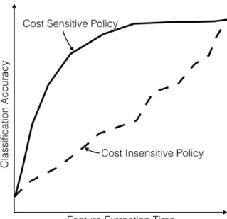
Figure 1: A notional plot highlighting the effect of cost sensitivity on anytime clas-sification accuracy. The solid curve corresponds to a cost sensitive policy, and the dotted curve a cost insensitive one. Both policies lead to the same accuracy once all features have been extracted, but the cost sensitive policy balances information with extraction cost to improve accuracy more quickly.

linearly with video length. For a 5 minute video recorded at 30 fps, computation can easily require an hour or more to extract flow-based features. Our method aims to reduce extraction time by only extracting features from the most important frames.

We ask the question, can we save time by extracting just a subset of the features while maintaining good classification accuracy? We answer this question by developing an anytime algorithm that sequentially extracts features. That is, for a given novel video that is to be classified, the algorithm dictates which feature to extract next during the sequential feature extraction process.

We refer to any such algorithm as a feature extraction policy. A policy thus implies an ordering over the features. The order in which features are extracted becomes important. For a given task, it is often the case that some features provide a larger boost to classification accuracy than others, whereas some features are less expensive to compute. Intuitively, a good policy should automatically manage the balance of these factors, selecting features in an order that increases classification accuracy most quickly. Figure 1 shows this idea graphically with a hypothetical Accuracy vs. Feature Extraction Time plot.

(8)

We formalize an abstraction for feature extraction policies and propose a novel implementation using a random forest variant, which we call a Frugal Forest. This policy is both cost-sensitive, meaning it takes into account how long each feature takes to extract; and dynamic, meaning it takes into account previously extracted feature values when estimating the usefulness of the remaining features.

Fundamentally, feature extraction policies are not new. Several works have investigated policies aimed at speeding up object detection and recognition in 2D im-ages (Gonzalez-Garciaet al., 2015, Alexeet al., 2012, Vijayanarasimhan and Kapoor, 2010, Karayevet al., 2012; 2014). In the video domain, Su and Grauman (2016) pro-pose a feature extraction policy for activity classification based on a Markov Decision Process (MDP), though it is not cost sensitive, and we show in several experiments that our Frugal Forest is empirically superior. The Feature-Budgeted Random Forest proposed by Nan et al. (2015) is both dynamic and cost sensitive but is fundamen-tally different from our model. The Feature-Budgeted Random Forest is not anytime, but instead learns a subset of features at training time and then extracts them all in batch at test time. The hope is that this subset will take less than the budgeted amount of time to extract, but this is not guaranteed. In contrast, our Frugal Forest has no notion of a budget at training time and will simply extract features at test time until it is stopped, allowing for anytime predictions.

We rigorously validate our model by subjecting it to a suite of six experiments. These experiments use two challenging datasets, one first-person and one third-person, that together contain more than 100 activity classes. The experiments also span a diverse set of feature spaces to further stress robustness. Our Frugal Forest policy surpasses or matches all baselines and the current state of the art for feature extraction ordering for activity classification, ultimately showing its effectiveness at balancing features’ predictive power with their cost.

2

Related Work

This section outlines previous work related to activity recognition and feature selection and is divided into four categories. Subsection 2.1 discusses activity recog-nition as a whole, without regard to feature extraction policies. Subsections 2.2 and 2.3 review works that aim to speed up computation on images for object localization

(9)

and recognition and on videos for activity detection and recognition, respectively. Lastly, subsection 2.4 looks at cost sensitive methods that include a notion of feature extraction cost.

2.1

Activity Recognition

Inferring a person’s action based solely on the frames of a video has proven to be quite challenging and has lead to a wide variety of approaches, as summarized in recent surveys (Turaga et al., 2008, Aggarwal and Ryoo, 2011). Several approaches use high level features such as objects or scenes for activity classification (Pirsiavash and Ramanan, 2012, Jain et al., 2015, Yao et al., 2011, Rohrbach et al., 2012, Han

et al., 2009). Other approaches use lower level features such as frame-level activation values from a CNN (Simonyan and Zisserman, 2014a, Xu et al., 2015, Zha et al., 2015).

There is a closely related problem called activity detection in which the video is not clipped to the extent of the activity, but rather the algorithm must localize the activity in space and time (Ke et al., 2005, Duchenne et al., 2009, Satkin and Hebert, 2010, Medioni et al., 2001, Yao et al., 2010, Kläser et al., 2010, Lan et al., 2011, Yu and Yuan, 2015, Jain et al., 2014, Gkioxari and Malik, 2015, Gemert et al., 2015, Chen and Grauman, 2012, Yuet al., 2011a). However, our method is restricted to recognition, and so we do not focus on detection works.

Activity recognition is a large field with many contributions, so we narrow our focus for the remainder of this subsection to Pirsiavash and Ramanan (2012), Soomro

et al. (2012) and Jain et al. (2015) which are most related to our work because we use their feature spaces and datasets.

Pirsiavash and Ramanan (2012) present the Activities of Daily Living (ADL) dataset, a collection of egocentric videos that show people performing activities of daily living. They propose a method for activity recognition that uses a bag-of-objects (BoO) histogram as features. They use the concept of a temporal pyramid which allows reasoning about the relative temporal distribution of objects. We also use this concept of dividing the video volume into regions.

Soomro et al. (2012) created the UCF101 dataset. With 101 activity classes and over 13,000 clips, it is larger and more realistic than most previous datasets. Jain et al.(2015) use the BoO feature space on this dataset with up to 15,000 object

(10)

classes. To our knowledge, Simonyan and Zisserman (2014a) achieve current state of the art classification accuracy on the UCF101 dataset by combining CNNs and dense trajectories.

Based on these recent successes, we evaluate our model in section 4 on two feature spaces: bag-of-objects histograms, and a “multi-feature” space comprised of combining multiple common feature types such as CNN activations, dense trajecto-ries, and more. In both cases, we extend the idea of the temporal pyramid and divide the video volume into a set of spatio-temporal regions, each of which contribute to the overall feature vector representation of the video clip to be classified.

Even though we draw inspiration from these closely related works, our work has a very different goal. The methods of these related works do not attempt to measure accuracy until all features have been extracted and therefore do not study a feature extraction policy. Our work is not a new approach to activity recognition, but to intelligent feature extraction.

2.2

Prioritizing Feature Computation in Images

There is a large body of work focused on reducing computation time for recog-nition in the image domain. Viola and Jones (2001) speed up object classification by extracting features in a cascade, quickly eliminating negatives. Pedersoli et al.

(2015) propose a coarse-to-fine approach for feature extraction for object detection in images. Others invent methods that operate only on small subsets of the image at a time (Gonzalez-Garcia et al., 2015, Alexe et al., 2012, Sadeghi and Forsyth, 2014, Dulac-Arnoldet al., 2013). Butko and Movellan (2009) design a method for searching for objects by maximizing expected information gain. Yu et al. (2011b) propose an active method for scene recognition. Vijayanarasimhan and Kapoor (2010) develop a dynamic feature prioritization method by applying a cost to each feature and estimat-ing the value of information (VOI) for each feature. Similarly, Gao and Koller (2011) develop a probabilistic method and assign costs to different classifiers. Karayev et al. (2012; 2014) present a cost sensitive reinforcement learning approach to anytime object recognition. We draw inspiration for a dynamic, cost-based system from these works in our extension to classification in the video domain.

(11)

2.3

Prioritizing Feature Computation in Video

An analogous body of work is concerned with reducing or prioritizing feature extraction in the video domain. Early detection or classification in video describes the problem of detecting or classifying an activity before the entire video is available. Methods from Ryoo (2011), Ryoo et al. (2014), Hoai and De la Torre (2014) are designed for streaming videos and involve collecting features before the video has completed. Our method also attempts to reason about the contents of the video before observing all features, but not in a streaming fashion. Rather, our method is designed for the batch setting, where it has access to the whole video and is free to jump forward and backward in time. Therefore our method does not attempt to solve early classification.

Yeunget al. (2016) propose an active method that selects the next frame of a video to analyze using a recurrent neural network in a batch setting, but this method is used for detection rather than recognition. Davis and Tyagi (2006) use an hidden Markov model (HMM) to determine a classification confidence and only continue to process frames until a desired confidence is achieved. Their method operates on sequential frames, though, which is different from an active policy like ours. Chen

et al. (2011) model a video using a chain graphical model and perform inference to determine which regions of the video deserve further computation. This model however, is not cost sensitive.

Su and Grauman (2016) develop a Q-learning approach that models the feature selection for activity classification problem as a Markov Decision Process (MDP). Their method learns a dynamic feature prioritization for activity recognition in both the streaming and batch domains. However, their method does not account for feature extraction costs and is not cost sensitive. While our idea could potentially also be implemented with an MDP, our random forest approach has the advantages of being quicker to train and easier to explain. That is, the tree structure makes it easy to understand why the model makes the choices it does. Furthermore, we demonstrate that our method competes well and improves over Su and Grauman (2016) when feature extraction costs vary.

(12)

2.4

Cost Sensitivity

Others have designed methods that take into account the cost of extracting features. The high level idea is to extract features that balance discriminative power with cost. Karasev et al. (2014) define the cost of evaluating a region of video to be proportional to its size. The overall score of the feature is its estimated predictive value minus its cost. This is similar our objective function. However, our method is different because we use random forests to learn a policy with the goal of activity classification whereas they take a VOI approach with the goal of video segmentation. Additionally, their method requires explicitly modeling conditional probability distri-butions and assumes objects to be spatially independent. Amer et al. (2012; 2013) use AND-OR graphs to evaluate videos in a cost sensitive way. This method also does not use random forests.

Nan et al. (2015) introduced feature budgeted random forests that also use a cost sensitive object function. Our method does not use the concept of a budget. Furthermore, their method fully traverses all trees at test time before providing a classification, and so is not anytime. Supplying a budget is a trade-off. Without a budget, the model greedily extracts features and allows the practitioner to stop the model and perform classification at any time. With a budget, however, the model can be less greedy and optimize for the specified budget. Additionally, a challenge with budgets, as noted by Nanet al. (2015), is training time only has expected costs of feature extraction and cannot guarantee it will meet the budget at test time.

Dredzeet al.(2007) develop a cost sensitive, mutual information-based method for quickly classifying email images as spam or not. Their MIt method sorts features

using a cost sensitive objective function for a fixed feature prioritization. Additionally, they invent a decision tree-based just-in-time (JIT) feature extraction policy that is both dynamic and cost sensitive. Their method, however, is not anytime, as the JIT feature extraction fully traverses the tree. Furthermore, the setting of email images provides metadata as features. Since metadata is far cheaper to compute than true visual features, their method ends up simply extracting metadata first. This makes sense for email image spam classification, but our activity recognition setting does not have this luxury.

(13)

3

Approach

This section describes our overall approach and details Frugal Forests. We first formalize feature extraction functions φj and spatio-temporal regions ri which

intuitively represent “what to look for” and “where to look for it in video space.” We then define the cost function which approximates the amount of time needed to extract a given feature φj over a region ri. We outline the anytime framework and

the general feature extraction policy abstraction it requires. We finish this section by describing our Frugal Forest policy and how it implements this general abstraction.

3.1

Augmented Feature Space

Let the unit cubeV represent the video we wish to classify to one activity class label ` ∈ L. Let φ be the function that maps V to its feature vector representation

f =φ(V), where f ∈_Rp_{. Let region} _r _{be a rectangular space-time volume where} _r

is a subset of V. Thus fi =φ(ri) is a feature vector representation of just the region

ri. Still, fi ∈ Rp. Let region set R = {ri : i = 0, ..., m} be a set of m regions. Let

the augmented feature vector f0 _∈

Rp·m _{be the concatenation of all} _f

i, i= 0, ..., m. A

classifierC :f0 _→_` _{maps an augmented feature vector to a single activity class label} `. The classifier is trained on a fully observed feature setf0_{. That is, all features have} been extracted.

Regions ri may vary in volume and shape, and may overlap with each other.

The intuition behind regions is they allow the classifier to leverage spatio-temporal correlations between features. Our method is agnostic to choice of feature space φ. Some concrete examples of features could be bag-of-object histograms (Pirsiavash and Ramanan, 2012, Jain et al., 2015), CNN activations (Krizhevsky et al., 2012), dense trajectories (Wang and Schmid, 2013), etc.

Note that φ might itself be logically composed of individual functions φj that

semantically extract different features. In the case of the BoO histogram feature space, the feature representation φ might be composed of one φj per object class,

each trained to detect a specific object. For example, a specific φj could correspond

to a “toothbrush” object detector, and φj(ri) means to run the toothbrush detector

(14)

3.2

Feature Extraction Cost

We model the cost of extracting a feature to be the amount of time required to compute the feature’s value. Since eachφj might intrinsically take a different amount

of time to compute, eachφj is associated with a respective cost factorcj. For example,

the feature space that is the combination of HOG features with HOF features, as in the approach of Laptev et al. (2008), might assign φ1 = HOG and φ2 = HOF with c1 < c2 because extracting optical flow-based HOF features is more expensive than extracting spatial gradient-based HOG features over the same region.

We reason that the cost of extracting a feature φj on some region ri is

pro-portional to the region’s volume Vol(ri) and the feature’s intrinsic cost cj. Many

common visual features (CNN activations, HOG, HOF, dense trajectories, etc.) rely on extraction techniques that require iterating over most or all pixels in the given region ri. The running time of such techniques increases with volume as they must

accommodate more pixels. Therefore, region volume is a good proxy for feature ex-traction time. One could extract features sparsely, only at space-time interest points. However, identifying the interest points requires operating over the whole image. Fur-thermore, dense features tend to give superior results to sparse, interest-point features (Wang et al., 2009).

During the process of extracting multiple features in sequence, it is possible to come upon a feature that has already been partially or totally computed. For example, suppose φj is an object detector with cj = 1, r1 is the full video volume, and r2 is

the first quarter of the video volume. That is, Vol(r1) = 1 and Vol(r2) = 0.25. If the system first invokes φj(r2), then it has already done 25% of the work of computing

φj(r1), and so Cost(φj, r1)should bediscounted to only the remaining 0.75. Likewise,

if instead φj(r1) was computed first, the cost of computing φj(r2) would be zero.

Formally, we define the discount factor d to be the percentage ofri that has already

been evaluated under φj.

(15)

3.3

Feature Extraction Policy

In general, a policy in our context is any algorithm that can supply to the system the “next” feature to extract. Thus the policy defines a sequential feature ordering.

In our framework, a generic policyπ has a training phase and a testing phase. During the training phase, the policy is allowed access to training data and the cost function. During the testing phase, the policy supports two operations: (1) the next

operation returns the feature index to be extracted next as an(i, j)tuple that specifies the desiredφj andri, and (2) theobserveoperation provides the policy an(i, j, φj(ri))

triple which can be recorded as part of the policy’s state and used by the policy to adapt to observed feature values on the fly. The testing phase framework is shown in algorithm 1. The loop condition is defined by the practitioner. Example conditions include a fixed amount of time, a fixed number of feature extractions, a classification confidence threshold, etc.

Algorithm 1 Testing phase framework

1: initialize f0 _←_{expected value}

2: repeat 3: (i, j)←π.next() 4: v ←φ_j(ri) 5: set(f0_{, i, j, v}₎ 6: π.observe(i, j, v) 7: yˆ←C(f0₎ 8: until < condition >

Feature values that have not yet been extracted are called missing. Initially, every feature value is missing. Missing values are temporarily assigned their respective expected value, as computed from training data. Once a feature’s true valuev =φj(ri)

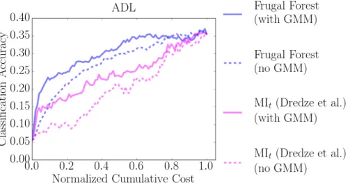
has been extracted, its entry inf0 _{is overwritten. Alternatively, missing values can be} imputed by more sophisticated models given the set of features extracted so far. We show that using a Gaussian Mixture Model (GMM) to impute missing values leads to higher classification accuracy. GMM imputation works as follows: Complete training data (no missing values) is clustered using ak-component GMM. At testing time, the missing values of an incomplete feature vectorf0_{are imputed to be a weighted average} of the GMM components where the weights are the normalized log probabilities that

(16)

the data pointf0

was generated by each component given the feature values extracted so far.

3.4

Frugal Forest Policy

We first describe the case of a single decision tree policy, then we describe how we extend to a forest policy.

A policy can be implemented as a binary1 _{decision tree where each node}

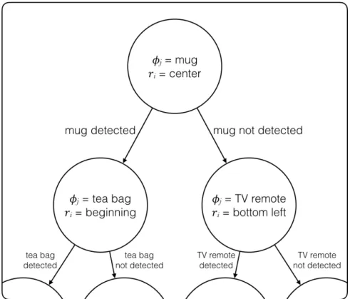
con-tains a feature index of the form(i, j), a scalar threshold t, a pointer to its left child, and a pointer to its right child. The feature ordering is defined by a traversal from the root node to a leaf node. Figure 2 shows an example decision tree that uses objects in the video as the features.

At training time, a node’s feature index (i, j) and threshold t are chosen to greedily maximize some objective function. For a traditional decision tree, this objec-tive function is information gain. We design a cost sensiobjec-tive objecobjec-tive function that accounts for feature extraction cost:

ObjFn(i, j, t) =InfoGain(i, j, t)−λCost(φj, ri) (2)

where λ∈_R is a scalar hyperparameter that governs the importance of cost relative to information gain and is chosen via validation data. This allows our policy to select features that balance predictive power with cost. For example, the feature with the highest information gain might be very expensive to compute, while a different feature might be cheap while still yielding decent information gain. The normal decision tree would simply always select the feature with highest information gain regardless of cost. We call trees trained with this modified objective function Frugal Trees.

At testing time, there is a notion of acurrent node nwhich is initialized to the root. When the next operation is invoked, the policy returns the feature index (i, j) of the current node n. When the observe operation is invoked with the argument

v =φj(ri), the policy compares v to the threshold t of the current node and updates

the current node to become its left child if v < t or its right child otherwise. This 1_{A tree of higher arity would work as well. Our binary tree logically accommodates non-binary}

features by allowing the same feature to be tested multiple times along a path from the root node to a leaf node.

(17)

Figure 2: Hypothetical portion of a decision tree policy where features are the presence or absence of objects in the video. Starting at the root node, the first feature selected is φj = “mug” at ri = the spatial center of the frames. If a mug is detected in this

region, the activity could likely be “making coffee” or “making tea,” as was learned during training. To reduce this uncertainty, the policy then selects to look for a tea bag near the temporal beginning of the video, having learned that tea bags usually appear at the start of the “making tea” activity. If instead a mug is not detected, it is likely the activity is one that does not involve a mug. The policy begins to investigate the plausibility of other activity classes by selecting to look for a “TV remote” in the bottom left region of the frames.

(18)

allows the policy to adjust the feature ordering as it gains information about the content of the video. Figure 2 shows an example decision tree policy that uses object presence or absence as features.

Our policy is implemented as a random forest, a collection of such decision trees. Following the usual random forest algorithm originally described by Breiman (2001), each tree is trained on a random sample of the training data and is restricted to a random sub-sample of the features. We call random forests that are composed of Frugal Trees as Frugal Forests.

With multiple trees, there are options when deciding how to traverse them at test time. We use a breadth-first traversal in which the forest maintains an array of

current nodes, one for each tree. Sequential calls to next cycle through the array of current node pointers, effectively letting the trees take turns. This is in contrast to a depth-first traversal in which the policy fully traverses one tree before moving on to the next. We choose to use the breadth-first traversal over depth-first because the experiments in subsection 4.6 show breadth-first as having a slight, if any, empirical edge over depth-first. We hypothesize this is because traversing deeper in the tree yields features that are more specific to the test instance at hand. Fitting to the test instance is precisely what we want at test time, but because of feature sub-sampling, the depth-first traversal begins fitting prematurely. The feature sub-sampling dur-ing forest traindur-ing encourages diversity among trees, and so a breadth-first traversal selects more general features first, allowing the policy to extract more general infor-mation about the test instance before diving deeper. In this sense, the depth-first traversal attempts to fit to the test instance too soon, whereas the breadth-first traversal immediately gets the benefits of feature sub-sampling.

It is worth reiterating that this forest policy does not perform classification, and so the trees do not vote or otherwise combine results. The forest only serves to order features during the sequential extraction process. A separate, potentially non-forest, classifier makes the activity class prediction. Our experiments use a logistic regression classifier, as described in section 4.

(19)

4

Results

This section is divided into 6 subsections. The first defines the baseline meth-ods to which we compare our model, and the rest present various experiments. Sub-section 4.2 defines the datasets and compares the anytime performance of our Frugal Forest policy to that of the baselines. Subsection 4.3 shows experiments that com-pare directly to the Q-Learning baseline of Su and Grauman (2016) by modifying the region setsR to match theirs. Since these region sets reduce cost variation, these ex-periments also serve as a stress test, introducing a situation where our method cannot benefit from cost sensitivity. Subsection 4.4 shows one experiment that mirrors one of the primary experiments but reduces the amount of cost variation available by using uniform cost factors cj. The experiments in subsection 4.5 explore the effects of

im-puting missing feature values. Finally, the experiments in subsection 4.6 investigate the differences in performance between depth-first and breadth-first forest traversals.

4.1

Baselines

1. Random Policy

The Random policy maintains a set S of unobserved features (i, j). The train

operation initializes S to be the set of all features. The next operation returns an element of S uniformly at random. The observe(i, j, v) operation removes element (i, j) from S and ignores v. This policy thus extracts features in a uniform random order.

2. MIt (Dredze et al.)

This is the MIt method proposed by Dredze et al. (2007) based on mutual

information. This policy maintains a queueQof unobserved features. Thetrain

operation initializes Q to be contain all features, sorted in ascending order of their score according to score(x) = (1−α)(1 −M I(x, y)) +α ×tx where x

is the feature, y is the label, M I is the mutual information function, tx is the

time required to extract featurex, and α is a hyperparameter that governs the trade off between mutual information and cost. Thenext operation returns the element (i, j) at the head of Q. The observe(i, j, v) operation pops the head element, which is enforced to be (i, j), fromQ and ignores v. This policy thus

(20)

extracts features in a meaningful and cost sensitive, but fixed order. 3. Vanilla Random Forest

The Vanilla Random Forest policy is a random forest whose trees are trained with the objective function that only maximizes information gain. The next

and observe operations are as defined in section 3.4. This policy thus extracts features in a meaningful and dynamic, but cost-insensitive order.

4. Q-Learning (Su et al.)

The Q-Learning policy of Su and Grauman (2016) models the problem as an MDP where each state s is a function of all observed feature values so far, and the action spaceA the set of all unobserved features(i, j). Thetrain operation implements Q-Learning to learn the Q function. The next operation returns the (i, j) action with the highest Q-value in the current state. The observe

operation implements the MDP transition from state s to the next state s0_. Similarly to the vanilla random forest policy, this Q-Learning policy extracts features in a meaningful and dynamic, but cost-insensitive order.

Our experiments vary in region set instantiation. Different region sets imply a different feature space f0_{. Therefore, models are not easily comparable across region} sets. The Q-Learning baseline was trained and evaluated using only the region sets of its original paper (Su and Grauman, 2016). Two of our experiments match these region sets. The others do not, and so the Q-Learning baseline is omitted there.

4.2

Primary Experiments

We validate our method against the baselines using three primary experiments. The first uses the Activities of Daily Living (ADL) dataset with a bag-of-objects his-togram (BoO) feature space where objects are detected using deformable parts models (DPM) (Pirsiavash and Ramanan, 2012). Activity classes are usually a function of the objects present, and more importantly, the objects interacted with. This is especially true for egocentric data because the camera does not observe most of the subject’s movements, and so common flow-based features are no longer effective. As shown by Pirsiavash and Ramanan (2012), the BoO feature space captures this object-centric relation well. The next experiment uses the UCF101 dataset (Soomro et al., 2012)

(21)

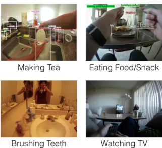
Figure 3: Example frames from the ADL dataset (Pirsiavash and Ramanan, 2012). In the top two frames, object classes and locations are annotated.

with a BoO feature space where objects are detected using a CNN (Jainet al., 2015). The last uses the UCF101 dataset with a “multi-feature” feature space that combines five common feature types, described in more detail later.

Experiment Setup

ADL: The ADL dataset (Pirsiavash and Ramanan, 2012) is a collection of egocentric videos from people wearing chest-mounted cameras performing activities of daily living. There are a total of 18 annotated activity classes, including “brushing teeth,” “doing laundry,” etc. There are 20 videos, each recorded by a different person, and each with multiple clips. Clips are pre-segmented to start and end with the activity. The authors of the dataset also provide DPM output for 26 object classes, including “microwave,” “tooth paste,” etc. Figure 3 shows example frames from the videos in this dataset.

Since each object class is extracted with a different DPM, we model each DPM as a function φj for j = 1, ...,26. We let costs cj = 1 for all j, assuming each DPM

takes roughly the same amount of time to run. Furthermore, following Yan et al.

(2014) we reason that about 30% of the computation of any DPM φj is low-level

image convolutions that can be shared across object classes j. The remaining 70% can only be shared within object classes.

(22)

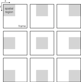
Figure 4: Nine of the ten spatial regions comprising S for the ADL dataset. Each white rectangle represents the full XY extent of a frame, and the gray rect-angle inside represents the extent of the spatial region si ∈ S. The one

spa-tial region not shown is the one that occupies the entire frame. This set of re-gions allows the policy to learn spatial correlations of objects at the granularity of {lef t, center, right} × {top, middle, bottom}. The regions overlap to prevent harsh boundaries between them that would prevent objects straddling such a boundary from being detected, essentially providing a small amount of spatial invariance, or “wiggle room.” The spatial region that covers the whole frame (not shown) is able to detect objects that are too large to fit within any of the other nine regions.

We define the region set R by first defining a spatial set S of 10 overlapping rectangles of varying size in the XY plane (see figure 4), and a temporal setT of seven overlapping intervals of varying size in the time dimension (see figure 5). The region setR is the cross product S×T. The total number of regions is|R|=|S| · |T|= 70, giving an overall augmented feature space of dimension dim(f0_{) = 26}_·_{70 = 1820.} Varying the size of the rectangles in S provides more information about the size and location of the object.

UCF (objects): The UCF101 dataset (Soomro et al., 2012) is comprised of 13320 YouTube clips, each belonging to one of 101 annotated activity classes. It is a challenging dataset for activity recognition with such a diverse set of activity classes. As with ADL, clips are pre-segmented to start and end with the activity. Figure 6

(23)

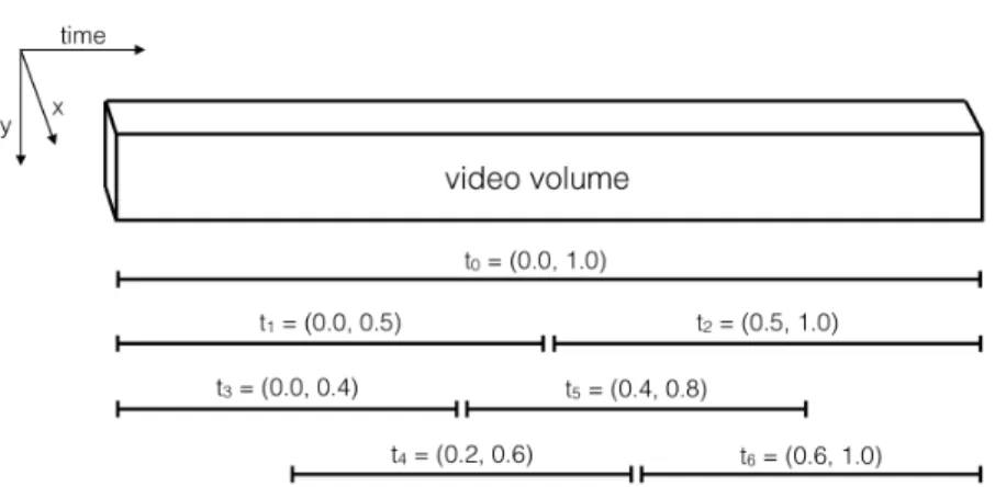
Figure 5: The seven temporal intervals comprising T for the ADL dataset. Values are in fractions of full video length. The first three intervals make up the temporal pyramid developed by Pirsiavash and Ramanan (2012). The four shorter intervals enable more fine grained temporal reasoning and allow the policy to reason about objects appearing only in the beginning, end, or middle of the video. For example, when the subject is making a sandwich, a “fridge” object might appear only at the beginning and end of the video when the subject gets out and puts away sandwich ingredients, but not during the middle of the video when the subject is making the sandwich. This pattern cannot be captured by the first three temporal intervals alone.

Figure 6: Example frames from the UCF101 dataset (Soomro et al., 2012). There is great diversity among activity classes.

(24)

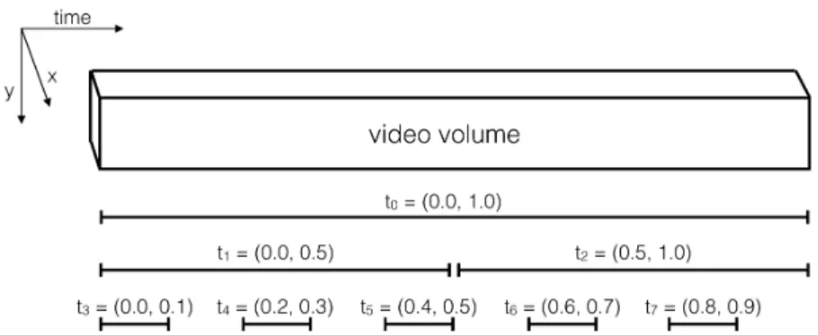
Figure 7: The eight temporal intervals comprisingR for the UCF101 dataset. Values are in fractions of full video length. As with the ADL dataset, we add to the temporal pyramid of Pirsiavash and Ramanan (2012) by including more fine grained temporal intervals. Here, the intervals are smaller than in the ADL case because videos of the UCF101 dataset are easier to classify correctly with fewer frames.

shows several example frames from this dataset.

Jainet al. (2015) present an activity recognition model trained on this dataset using the familiar bag-of-objects histogram feature space. They provide object detec-tor outputs for 15,000 object classes, but we use their method of identifying “preferred objects” to reduce this to only the 75 most preferred object classes. As described by Jain et al. (2015), the idea behind “preferred objects” is that not all 15,000 object classes are needed for a maximally discriminative representation. Instead, each ac-tivity class is associated with a subset of k object categories. For each activity class, its “preferred” objects are those that are most responsive. The total set of preferred objects is the union over activity classes of these subsets.

Unlike with the ADL dataset, here objects are detected with a CNN. Specifi-cally, we use the fc-7 layer activations of VGG-16 (Simonyan and Zisserman, 2014b). Since the CNN detects all objects simultaneously, there is only one feature extraction function φ, and we let its corresponding cost factor c be 1. Since the CNN operates on the whole image, all regionsri span the full XY extent of the video, and so regions

only vary along the temporal dimension. We use a region setR with 8 regions, again overlapping and of varying size (see figure 7). Thus dim(f0_{) = 75}_·_{8 = 600. But} each invocation ofφ yields 75 values (one per object class), so the policy only reasons about 8 actions(i, j).

UCF (multi-feature): This experiment uses the same UCF101 dataset but a different feature space that is a concatenation of fivefeature types:

(25)

1. CNN activations from the fc-7 layer of VGG-16 (Simonyan and Zisserman, 2014b), averaged over time (4096 dimensions). This feature type captures high-level features that are indicative of ImageNet object classes (because this net-work was trained on ImageNet).

2. Bag-of-HOG histogram (Laptev et al., 2008) (4000 dimensions). This feature type captures low-level spatial structure.

3. Bag-of-HOF histogram (Laptev et al., 2008) (4000 dimensions). This feature type captures low-level temporal motion.

4. Bag-of-MBH histogram (Wang and Schmid, 2013) (4000 dimensions). This feature type captures relative motion between entities in the video.

5. Bag-of- Dense Trajectories (DT) histogram (Wang et al., 2013) (4000 dimen-sions). This feature type captures mid-level spatio-temporal video dynamics.

To reduce dimensionality, we apply PCA to each of the five feature types in-dependently, keeping only the 100 largest components of each. Concatenation results in only 500 dimensions. We refer to this feature space as “multi-feature.”

We use the same 8 regions as in the previously described experiment, shown in figure 7 . Thus, dim(f0_{) = 500}_·_{8 = 4000. There is one feature extraction function} φj for each feature type. Each invocation of a function φj yields a vector of feature

values φj(ri) = v ∈R100. The action space of the policy thus has size 5·8 = 40.

Assigning values to the cost factors cj of the different feature types is not

straightforward, in part because the time required to extract such features depends on several hyperparameters (e.g. bin size for HOG). We use the relative ordering HOG < MBH < HOF < CNN < DT based on the following logic: HOF, MBH, and DT require expensive optical flow computation. HOF and MBH are similar in cost, while DT is the most expensive because it requires tracking post processing. HOG only requires a small number of convolutions per image, so it is the cheapest. A forward pass of VGG-16 incurs thousands of convolutions per frame (Simonyan and Zisserman, 2014b), expensive enough to surpass optical flow. Accordingly, we come up with a reasonable set of cost factors~c= (6,1,4,3,10) (order is the same as the ordered list above, i.e. HOG is the cheapest and dense trajectories are the most expensive).

(26)

Since cost sensitivity is an advantage for our Frugal Forest method, larger variance among the cost factors cj should be best handled by our method. We test

this theory, and the robustness of our method, with the experiment in subsection 4.4 in which all cost factors are set to cj = 1.

Implementation Details

Both the Vanilla Forest and the Frugal Forest were composed of 80 trees. When training the forests, each tree was exposed to a random subset of 160 features during the ADL and UCF (objects) experiments, and 2000 features for the UCF (multi-feature) experiment. The Frugal Forest was trained with λ = 0.4. The MIt model

was trained withα = 0.5. Missing feature values were imputed with a 10-component GMM for the ADL and UCF (objects) experiments, and a 100-component GMM for the UCF (multi-feature) experiment. All of these parameters were chosen via validation data. The classifier was a logistic regression model. The GMM and the classifier were trained on fully-observed training data (no missing values). We perform cross validation with splits recommended by the respective datasets. Accuracy is measured as the mean along the diagonal of the classification confusion matrix.

Results

Figure 8 shows the results of these three experiments in the form of Classi-fication Accuracy vs Normalized Cumulative Cost plots, where cost is a proxy for computation time. Notice that every curve starts and ends at the same points. These points correspond to when no features have yet been extracted, and when every feature has been extracted. In these cases, the classifier will give the same result regardless of policy.

The rest of this section is split into three parts, each evaluating the results of the respective three plots.

ADL: Figure 8a shows results for the ADL experiment. Our Frugal Forest has the fastest gain in accuracy. The Vanilla Forest has similar accuracy after a cumulative cost of around 0.2, but the Frugal Forest is more accurate at the very beginning. When the Frugal Forest attains an accuracy of 20%, the Vanilla Forest attains an accuracy of about 16%.

(27)

0.0 0.2 0.4 0.6 0.8 1.0 Normalized Cumulative Cost 0.00 0.05 0.10 0.15 0.20 0.25 0.30 0.35 0.40 Classification Accuracy ADL Frugal Forest Vanilla Forest MIt (Dredze et al.) Random

(a) Primary experiment with the ADL dataset and BoO feature space. This experiment emphasizes the importance of being dynamic.

0.0 0.2 0.4 0.6 0.8 1.0

Normalized Cumulative Cost 0.0 0.1 0.2 0.3 0.4 0.5 Classification Accuracy UCF (objects) Frugal Forest Vanilla Forest MIt (Dredze et al.) Random

(b) Primary experiment with the UCF101 dataset and BoO feature space. This experiment emphasizes the importance of being cost sensitive.

(28)

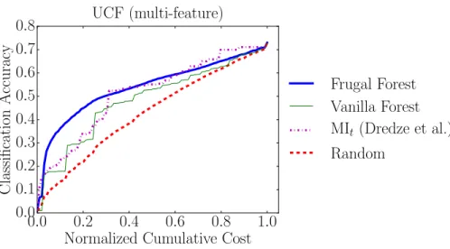
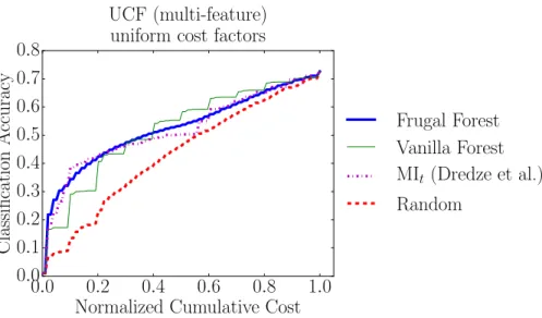
0.0 0.2 0.4 0.6 0.8 1.0 Normalized Cumulative Cost 0.0 0.1 0.2 0.3 0.4 0.5 0.6 0.7 0.8 Classification Accuracy UCF (multi-feature) Frugal Forest Vanilla Forest MIt (Dredze et al.) Random

(c) Primary experiment with the UCF101 dataset and multi-feature space. This experiment emphasizes the importance of being both dynamic and cost sensitive.

Figure 8: Results from primary experiments, spanning two challenging datasets and two different feature spaces. In all cases, our Frugal Forest policy exceeds or matches all baselines, showing the power of combining cost sensitivity with being dynamic.

A perhaps surprising result is that the Random policy is competitive with MIt.

This is caused by two reasons, both specific to the dataset. The first is that mutual information is not a good metric for selecting features on the ADL dataset because the same objects are commonly seen across different activity classes. Intuitively, detecting the object class “mug” is not enough to be certain of the activity class because many activities could feasibly include a mug, including “washing dishes,” “moving dishes,” “making tea,” “making coffee,” and “drinking coffee/tea.” Or perhaps the person is performing an unrelated activity and the mug happens to be visible in the background. The key to doing well on this dataset is effectively modeling the spatio-temporal relationship between objects. For example, if the mug is present in the center of the frame for the majority of the video while a tea bag is present only briefly near the beginning of the video, then it becomes more likely the person is “making tea.” The downfall of mutual information here is that it does not capture relationships between objects, but rather scores each object independently. A tree structure captures these relationships well, each node conditioning on the objects detected or not detected in its ancestor nodes, leading the two forest methods to their superior performance.

(29)

The second reason is that cost sensitivity only plays a minor role in perfor-mance with this dataset. On top of this, the Random policy happens to select cheap features more often than expensive ones because there are more cheap features avail-able than expensive ones, further reducing the cost sensitivity benefit the MIt policy

has over the Random policy. Indeed, the cost insensitive Vanilla Forest policy does nearly as well as its cost sensitive Frugal Forest counterpart, further supporting the claim that cost sensitivity does not play as important a role with this dataset as with others.

UCF (objects): Figure 8b shows the results for the UCF (objects) experi-ment. Our Frugal Forest method is again the best policy, but the plot overall looks quite different from the ADL experiment. The “step-like” shape of the curves show that classification accuracy remains constant until more features become available. The “steps” do not appear in the ADL experiment because it uses finer-granularity features and costs, a byproduct of its larger region set R and more feature extractor typesφj.

The Frugal Forest and MIt policies do particularly well here, balancing cost

with predictive power. These two models nearly match each other while the Vanilla Forest does quite poorly, suggesting cost sensitivity is more important than being dynamic for this particular dataset and feature space. This result is opposite the one observed in the ADL experiment and can likewise be explained by the nature of the datasets. The videos in the UCF101 dataset are short, and the activities are very distinct from one another, e.g. “lifting weights” vs. “surfing” vs. “haircut” etc. Here, detecting just one object can be enough to correctly infer the activity. For example, detecting the object class “barbell” in a single frame is likely sufficient to correctly classify the video clip as “lifting weights.” Moreover, the video settings are all different, so we don’t see extraneous objects in the background of the video like we see in the ADL dataset.

Notice that Random does much better than the Vanilla Forest. As in the previous experiment, there are more cheap features to choose from than expensive features. Consequently, the Random policy happens to select cheap features quite often. In this experiment, there are five “cheap” features (i, j) that each cost 0.1, meaning the volume of their region is Vol(ri) = 0.1; two “expensive” features that

(30)

very expensive feature that costs 1.0, where the region is the whole video volume. This leads the Random policy to outperform the more sophisticated Vanilla Forest policy, which selects the more expensive features due to their higher predictive power. Indeed, the Vanilla Forest curve remains near zero until normalized cumulative cost reaches 0.5, indicating the first feature extracted was expensive for most cross validation folds. UCF (multi-feature)Figure 8c shows the results for the UCF (multi-feature) experiment. Again, our Frugal Forest policy is the best, this time with a more pro-nounced lead over the baselines in the beginning. The MItbaseline catches up to our

Frugal Forest at around a normalized cumulative cost of 0.3, and even briefly exceeds it near the end.

This combination of dataset and feature space provides roughly equal benefit to cost sensitivity and to being dynamic. This claim is supported by the fact that the cost sensitive MIt policy roughly matches the dynamic Vanilla Forest. The Random

policy, which is neither cost sensitive nor dynamic, is the worst policy of the four, achieving the lowest classification accuracy per unit time. Our Frugal Forest realizes both benefits, exceeding all baselines by a clear margin in the beginning. Compared to the previous UCF (objects) experiment, this new feature space invalidates the “one feature is enough” property. Rather, the result of extracting one feature value v = φj(i, j) allows the policy to make important adjustments, as was the case with

the ADL experiment. However, the degree to which this is important is not as high as in ADL. This experiment can be viewed as a middle ground between the first two experiments with respect to the importance of cost sensitivity and being dynamic.

Finally, notice that overall accuracy jumps from about 0.5 in the previous experiment to about 0.7 in this one. This supports the idea that more complex feature spaces can indeed be effective and necessary, and that it is not always sufficient to settle for faster, simpler features.

It is worth pointing out that the final accuracies (when all features are ex-tracted) reported in this work do not beat the current state of the art, as Pirsiavash and Ramanan (2012) and McCandless and Grauman (2013) achieve higher overall accuracy on the ADL dataset, and Jain et al. (2015) and Simonyan and Zisserman (2014a) achieve higher overall accuracy on the UCF101 dataset. Final accuracy is not the metric of concern here, as it is not a function of the feature extraction policy. Rather, our goal is to improve accuracy when only a fraction of all features can be

(31)

extracted.

These experiments show the benefits a feature extraction policy can gain from being dynamic, from being cost sensitive, and from being both. Our proposed ap-proach combines these two crucial ingredients to produce a feature extraction policy that effectively selects the “right” features when needed regardless of dataset or feature space.

4.3

Comparison to Q-Learning (Su and Grauman)

We perform two experiments in this subsection that directly compare our Fru-gal Forest model to the Q-learning model of Su and Grauman (2016). To properly compare our two respective policies, we must use the same feature space. This means using the same set of featuresφj and regionsri. Therefore we modify our experiments

to match those of Su and Grauman (2016). In both experiments, the region set used are defined such that regions ri do not overlap. This greatly reduces cost variation

among features, preventing our Frugal Forest from realizing its cost sensitivity ad-vantage. Even under these inherently cost-insensitive conditions, our method still outperforms the baselines.

Experiment Setup

The first of the two experiments is analogous to the primary experiment shown in figure 8a. It uses the ADL dataset and the BoO feature space, but defines the region set by dividing the video volume into a uniform grid, splitting each video dimension into two halves. This gives a total of eight equally sized and non-overlapping regions, each with Vol(ri) = 1₈. We denote this volume division as the “2x2x2” pattern.

The second experiment is analogous to the primary experiment shown in figure 8b. It uses the UCF101 dataset and BoO feature space, but defines the region set by dividing the video volume into fourths along the time dimension. Regions still span the full extent of the X and Y dimensions because objects are detected using a CNN which requires a fixed image width and height. This results in a total of four equally sized and non-overlapping regions ri, each with Vol(ri) = 1₄. We denote this volume

(32)

Results

Like in subsection 4.2, we present results and analysis for each of the two experiments separately.

ADL: Figure 9a shows results for the ADL experiment on the “2x2x2” region set, comparing against the existing Q-Learning approach. Uniform sized regions together with uniform cost factors cj = 1 means the cost of extraction is the same

for every feature, before discounting is applied. Non-overlapping regions implies that any non-zero discount can only arise from running different DPM object detectors φj over the same region ri. Recall there is a 30% discount when running a DPM

over a region that has already been evaluated by a different DPM because low level convolutions can be shared (Yanet al., 2014). All of this together implies that there is very little cost variation to be exploited, especially at the beginning of the feature extraction process. This is why the Vanilla Forest matches our Frugal Forest in the beginning, and nearly matches it throughout.

The explanation for the poor performance of MIt is the same as before: the

ADL dataset rewards dynamic polices more than cost sensitive ones.

The Q-Learning policy falls well below both forest polices despite its dynamic nature. It matches the forests only at the very beginning and diverges when classifi-cation accuracy reaches about 15%.

It is also important to notice the drop in final classification accuracy compared to the primary ADL experiment in subsection 4.2 (30% vs. 35%). This is evidence that the richer representation provided by the overlapping and non-uniform region set is indeed helpful.

UCF (objects): Figure 9b shows results for the ADL experiment on the “1x1x4” region set. This experiment is even more extreme, fully eliminating all cost variation. This takes away all cost-sensitive advantages of the Frugal Forest and logically reduces it to a Vanilla Forest. Similarly, the MIt policy becomes equivalent

to a policy that simply ordering features by their mutual information score with respect to the labels, ignoring cost. Additionally, this setup has only one feature extraction function φ (i.e. the CNN) and four regions ri, leading to a total of only 4

features (i, j) the policy has to choose from. This reduction in action space reduces the advantage our Frugal Forest gets from its being dynamic.

(33)

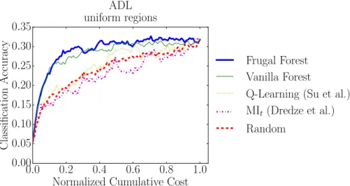
0.0 0.2 0.4 0.6 0.8 1.0 Normalized Cumulative Cost 0.00 0.05 0.10 0.15 0.20 0.25 0.30 0.35 Classification Accuracy ADL uniform regions Frugal Forest Vanilla Forest

Q-Learning (Su et al.)

MIt (Dredze et al.)

Random

(a) Experiment with the ADL dataset, BoO feature space, and the “2x2x2” region set of Su and Grauman (2016).

0.0 0.2 0.4 0.6 0.8 1.0

Normalized Cumulative Cost 0.0 0.1 0.2 0.3 0.4 0.5 Classification Accuracy UCF (objects) uniform regions Frugal Forest Vanilla Forest

Q-Learning (Su et al.) MIt (Dredze et al.)

Random

(b) Experiment with the UCF101 dataset, BoO feature space, and the “1x1x4” region set of Su and Grauman (2016).

Figure 9: Results from two experiments comparing directly against the Q-Learning method of Su and Grauman (2016). The modified regions hinder our Frugal Forest method’s ability to leverage cost sensitivity. Still, our method matches or exceeds all other methods.

(34)

policy matches the forests until the last fourth of the feature extraction process, sug-gesting either the advantage of being dynamic is not totally gone, or that information gain happened to be a better metric than mutual information in this case. Random is slightly worse than the other baselines, proving that the order in which these features are extracted still matters.

With the dynamic aspect diminished and cost sensitivity fully eliminated, this experiment represents the “worst case” scenario for Frugal Forests. Yet, even under these extreme conditions, Frugal Forests do not become worse than other methods. Because our method’s foundation is information gain, it still produces a good fea-ture ordering, even after the benefits of being dynamic and cost sensitive have been stripped away.

4.4

Multi-Features with Uniform Cost Factors

Since cost sensitivity is an advantage for our Frugal Forest method, larger variance among the cost factors cj should be best handled by our method. We test

this theory, and the robustness of our method, with an experiment in which all cost factors are set to cj = 1.

Experiment Setup

The experiment setup is identical to the previous experiment that uses the UCF101 dataset with the “multi-feature” feature space, shown in figure 8c, except that all five cost factors are set to the same value. This setup removes the cost variation due to cost factors cj, but not the cost variation due to the non-uniform,

overlapping region set. So overall cost variation is reduced but not eliminated.

Results

Figure 10 shows results for this experiment. Still, no baseline outperforms our Frugal Forest in the beginning. The margin between our Frugal Forest and the baselines is smaller than in the corresponding primary experiment using non-uniform cost factors, shown in figure 8c. This smaller margin is caused by the reduction in cost variation exploitable by our Frugal Forest policy.

(35)

0.0 0.2 0.4 0.6 0.8 1.0 Normalized Cumulative Cost 0.0 0.1 0.2 0.3 0.4 0.5 0.6 0.7 0.8 Classification Accuracy UCF (multi-feature) uniform cost factors

Frugal Forest Vanilla Forest MIt (Dredze et al.)

Random

Figure 10: Experiment with the UCF101 dataset using the “multi-feature” feature space. All five feature types have the same cost factor cj = 1. This reduces the

benefit of cost sensitivity, which is why our Frugal Forest policy leads by a smaller margin than in the corresponding experiment that used non-uniform cost factors, shown in figure 8c.

After about half way through the feature extraction process, the Vanilla Forest begins to outperform the Frugal Forest. One possible explanation for this phenomenon is that, in cases when cost plays a lesser role, as in this experiment, investing in the more expensive features can lead to higher classification accuracy later on.

Notice that the Vanilla Forest also outperforms the cost sensitive MItbaseline

toward the end of the feature extraction process, unlike in the non-uniform cost experiment. This further supports the reasoning that cost sensitivity is the reason that the Frugal Forest and MIt policies fall behind the Vanilla Forest policy near the

end of the process.

Identifying the “best” policy in this case depends on how much computation is allowed. The Frugal Forest policy selects features to optimize accuracy for less computation. In this case, the Frugal Forest policy is the better choice if less than half of the features can be extracted. On the other hand, if more than half of the features can be afforded, then the cost-insensitive Vanilla Forest policy would be the better choice.

As a reminder, the goal of this work is to achieve good classification accuracy while using just a fraction of computation required to extract all features. Under this

(36)

light, this experiment reinforces the usefulness of the Frugal Forest policy and cost sensitivity in general.

4.5

Imputation Experiment

This experiment explores the effect of imputing missing values. Specifically, we compare GMM imputation to the less sophisticated method of just using the missing feature’s expected value.

Experiment Setup

The experiment setup is the same as the first two primary experiments de-scribed in subsection 4.2. The first uses the ADL dataset with the BoO feature space. The second uses the UCF101 dataset with the BoO feature space.

Results

Figure 11 shows the results of this experiment. All policies benefit from GMM imputation over mean imputation. This shows that the more sophisticated GMM imputation method provides better estimates of missing feature values, in turn im-proving intermediate classification accuracy.

4.6

Forest Traversal Experiments

This experiment aims to explain why the breadth-first forest traversal might perform better than depth-first. We run three experiments that evaluate our Frugal Forest policy under both breadth-first and depth-first scenarios.

Experiment Setup

The experiment setup is the same as the primary experiments described in 4.2. The first uses the ADL dataset with the BoO feature space. The second uses the UCF101 dataset with the BoO feature space. The third uses the UCF101 dataset with the “multi-feature” feature space.

(37)

Figure 11: Experiment showing the effect of GMM imputation for missing feature values on anytime classification accuracy. Solid curves use GMM imputation whereas dashed curves use the simpler mean imputation. All policies benefit roughly equally from GMM imputation, so some policies are omitted from the plot to prevent the plots from becoming too cluttered.

(38)

(a) Experiment showing a small difference between breadth-first and depth-first forest traversals on the ADL dataset using the BoO feature space.

(b) Experiment showing breadth-first and depth-first forest traversals give identical results on the UCF101 dataset using the BoO feature space.

(39)

(c) Experiment showing breadth-first and depth-first forest traversals give identical results on the UCF101 dataset using the “multi-feature” feature space.

Figure 12: Experiment showing the breadth-first forest traversal having a slight edge, if any, over the depth-first traversal on the ADL dataset, but showing no difference between the two traversals on the UCF101 dataset. This leads to the conclusion that the optimal traversal method is dependent on dataset.

Results

Figure 12 shows the results of rerunning the three primary experiments with both breadth-first and depth-first traversals of our Frugal Forest policy. The ADL experiment shown in 12a displays a small difference in classification accuracy be-tween the two traversals in the beginning. The UCF experiments, however, show no difference in classification accuracy at all between the two traversals.

To understand why the two traversal methods produce a difference in the ADL experiment but not the UCF experiment, recall an important difference between these two datasets: The UCF101 dataset has the “one object is enough” property, where the one-to-one correspondence between object presence and activity class is high. This property applies to the “multi-feature” case, too, in that extracting one highly responsive flow descriptor could be enough to reveal the activity class, for example. In contrast, objects in the ADL dataset are often present in multiple activity classes. This is because the same objects are used across activity classes and because irrelevant

(40)

objects can be seen in the background.

We interpret the process of traversing down a single tree as refining the current belief about the content of the video and its activity class. Intuitively, the tree “narrows in” on a certain activity class, or group of related activity classes, as it travels from root to leaf.

With the “one object is enough” property in mind, it makes sense that the early refinement of the depth-first forest traversal doesn’t hurt accuracy. The policy will iterate through objects until it detects one, at which point there is enough confidence to begin refinement. The opposite is true for the ADL experiment. If the policy begins narrowing in immediately, it selects features that turn out not to be as helpful as the more exploratory features selected by the breadth-first traversal.

Though the empirical difference between the two traversal methods is small, it is robust to changes in hyperparameter values. Varying the number of trees in the forest and the number of sub-sampled features per tree produces a similar result.

5

Conclusion

Our work is motivated by the fact that visual features for activity classifica-tion are computaclassifica-tionally expensive to compute. Furthermore, the current trends in the literature suggest that features are becoming even more expensive as yet more complex video representations lead to higher classification accuracy. Some real-world applications cannot afford to extract all features. We attempt to solve this problem by learning an anytime feature extraction policy that will select features for on-demand extraction in a sequence that increases classification accuracy most quickly. We pro-pose the Frugal Forest as a feature extraction policy that is both dynamic, observing extracted feature values and adapting to new information on the fly; and cost sensi-tive, balancing a feature’s estimated informative value with its extraction cost. These two properties together allow our Frugal Forest to achieve better activity classification accuracy per unit time than other methods.

We conducted experiments across two prominent and difficult activity recog-nition datasets and used a variety of different visual features. These experiments showed our Frugal Forest exceeding or matching all baselines. In addition, we con-ducted experiments that show our Frugal Forest policy is resilient to “worst case”

(41)

situations that reduce or eliminate cost variation among features.

We showed that imputing missing feature values helps improve accuracy per unit cost, comparing Gaussian Mixture Model (GMM) imputation to the simpler mean imputation.

Lastly, we investigated the difference between breadth-first and depth-first forest traversals and their effect on anytime classification accuracy. We hypothesized that a breadth-first traversal selects more exploratory features in the beginning of the feature extraction process, whereas a depth-first traversal will quickly refine the current belief. The more exploratory breadth-first method showed to be slightly more beneficial for the ALD dataset while the UCF101 dataset showed no difference because of its “one object is enough” property.

In conclusion, our Frugal Forest feature extraction policy attains the highest anytime classification accuracy per unit cost of all our baselines, including the current state of the art. The superior performance is attributed to two properties: being dynamic, and cost sensitivity.

Future work might investigate the use of gradient boosted trees which have shown promising results (Friedman, 2001) and might make for a better feature extrac-tion policy than a random forest. One practical difference between gradient boosted trees and random forests is that gradient boosted trees cannot be trained in parallel because each successive tree depends on the previous ones, whereas the trees of a ran-dom forest can be trained independently. This will likely lead to increased training time, however training time is usually of small concern relative to test time accuracy. Another avenue of potential future work would be to apply Frugal Forests to the streaming domain, where the policy does not have access to the whole video and thus cannot jump forward in time. Such a scenario would require modifying the training algorithm so that tree nodes only select regions of video that are estimated to be available by the time that node is reached during test time. This begs the question, how should the test time framework respond when the policy selects a video region that is not yet available? A naive solution would have the system block until the selected video region becomes available, but this approach has the obvious drawback of sitting idle. An alternative test-time solution could be to skip nodes that select unavailable video regions, putting such nodes in a queue and coming back to them later.

(42)

After researching the potential impact that dynamic and cost sensitive meth-ods can have on anytime classification, we are excited to see further advances in the future.

(43)

Bibliography

Jake K Aggarwal and Michael S Ryoo. Human activity analysis: A review. ACM Computing Surveys (CSUR), 43(3):16, 2011.

Bogdan Alexe, Nicolas Heess, Yee W Teh, and Vittorio Ferrari. Searching for objects driven by context. In Advances in Neural Information Processing Systems, pages 881–889, 2012.

Mohamed Amer, Dan Xie, Mingtian Zhao, Sinisa Todorovic, and Song-Chun Zhu. Cost-sensitive top-down/bottom-up inference for multiscale activity recognition.

Computer Vision–ECCV 2012, pages 187–200, 2012.

Mohamed R Amer, Sinisa Todorovic, Alan Fern, and Song-Chun Zhu. Monte carlo tree search for scheduling activity recognition. In Proceedings of the IEEE Inter-national Conference on Computer Vision, pages 1353–1360, 2013.

Leo Breiman. Random forests. Machine learning, 45(1):5–32, 2001.

Nicholas J Butko and Javier R Movellan. Optimal scanning for faster object detection. In Computer vision and pattern recognition, 2009. cvpr 2009. ieee conference on, pages 2751–2758. IEEE, 2009.

Chao-Yeh Chen and Kristen Grauman. Efficient activity detection with max-subgraph search. InComputer Vision and Pattern Recognition (CVPR), 2012 IEEE Confer-ence on, pages 1274–1281. IEEE, 2012.

Daozheng Chen, Mustafa Bilgic, Lise Getoor, and David Jacobs. Dynamic processing allocation in video.IEEE transactions on pattern analysis and machine intelligence, 33(11):2174–2187, 20