Predicting Extreme Returns in the Canadian Stock Market

(1)

Predicting Extreme Returns in the Canadian

Stock Market

A Thesis in the

John Molson School of Business

For the Degree of

Master of Science (Finance option) at Concordia University

Montreal, Quebec, Canada

March 2016

(2)

CONCORDIA UNIVERSITY School of Graduate Studies

This is to certify that the thesis prepared By: Yun Zhao

Entitled: Predicting Extreme Returns in the Canadian Stock Market and submitted in partial fulfillment of the requirements for the degree of

Master of Science (Finance option)

complies with the regulations of the University and meets the accepted standards with respect to originality and quality.

Signed by the final Examining Committee:

Chair: Pierre-Yann Dolbec Examiner: Ravi Mateti Examiner: Alan Hochstein Supervisor: Lorne N. Switzer Approved by

(3)

iii

Abstract

Expecting Extreme Returns in the Canadian Stock Market Yun Zhao

This study examines the relationship between volatility and the probability of occurrence of expected extreme returns in the Canadian market. Three measures of volatility are examined: implied volatility from firm option prices, conditional volatility calculated using an EGARCH model and idiosyncratic volatility based on the Fama and French five-factor model. A significantly positive relationship is observed between a firm’s idiosyncratic volatility and the probability of occurrence of an extreme return in the subsequent month for firms. A 10% increase in idiosyncratic volatility in a given month is associated with the probability of an extreme shock in the subsequent month (top or bottom 1.5% of the returns distribution) of 26.4%. Other firm characteristics, including firm age, price, volume and Book-to-Market ratio, are also shown to be significantly related to subsequent firm extreme returns. The effects of conditional and implied volatility are mixed.

Keywords: Extreme return; Implied volatility; Conditional volatility; Idiosyncratic volatility; Five-Factor model; Probit regression;

(4)

1. Introduction

The study of extreme returns has been of increased interest to researchers and practitioners in recent years. Analyzing extreme returns is important because of their potential to explain investor behavior. For example, Switzer, Lee, Zhao and Yang (2015) demonstrate that extreme-day measure better explains the behavior of loss averse investors than traditional standard deviation proxy for Canadian and U.S. investors. An (2015) also finds that investors sell more when they have stocks with both larger unrealized gains and larger unrealized losses. Because the higher selling pressure of stocks with extreme returns leads to lower current prices and higher future returns, such investor’s trading behavior can affect equilibrium price dynamics. There are also studies showing the importance of identifying extreme return firms for filtering out outliers from value-weighted market positions. Fodor, Krieger, Mauck, and Stevenson (2013) demonstrate that, in the U.S. market, when the ex ante (predicted) extreme return stocks are removed from a portfolio, the betas decrease and the overall portfolio performance actually improves. Identifying and excluding predicting extreme return firms is therefore a challenge, but may be of great importance for investors. The purpose of this study is to try to identify factors that may be helpful in predicting extreme returns in the Canadian stock market.

Most extant work in this area looks at US markets. Fodor, Krieger, Mauck, and Stevenson (2013) show positive relationship between implied volatility from option price in U.S. market. This study extends Fodor, Krieger, Mauck, and Stevenson (2013) by looking at the extreme return predictive ability of implied volatility from option prices, as well as from conditional volatility calculated from an EGARCH model, and idiosyncratic volatility calculated by using the Fama and French (2015) five-factor model.

This paper sheds new light on the predictive ability of idiosyncratic volatility based on the Fama and French (2015) five-factor model for expected returns. Fama and French (2015) suggest that their five-factor model, which captures the size, value, profitability, and investment patterns

(6)

2

in average stock returns performs better than their widely used three-factor model (Fama and French (1993)).

Other explanatory factors, which are shown to have predictive ability for extreme returns in past research, are also included in this study. These factors include: firm size, book-to-market ratios, trading volume and equity price. This paper aims to investigate the incremental effects of these variables on probability of occurrence of expected extreme returns, controlling for the effects of idiosyncratic volatility.

This study focuses on firm data in Canadian stock market, from 2001 to 2014. Probit regression models are estimated to identify the relationship between the probability of occurrence of expected extreme returns and firm characteristics. The Fama-Macbeth procedure is used to calculate the model coefficients and Newey-West standard errors coefficients are used to calculate t-statistics. This study is conducted for the market as a whole, as well as for firms in the natural resource industry, an important sector for the Canadian economy as a whole, which has experienced considerable volatility in recent years.

In this paper, three measures of volatility are tested in our probit regressions, which are designed to forecast the probability of extreme return behavior. The first model uses implied vitality from option prices. The second model uses conditional volatility from an E-GARCH model. The third measure is the idiosyncratic volatility measured using the Fama and French (2015) five factor model. The models are estimated over three samples: 1. The Canadian market as a whole. 2. A subsample of the market consisting of firms in the natural resource sector; 3. A subsample of the market consisting of non-natural resource firms. A number of alternative classifications of extreme events are also considered in the analyses.

This paper serves to contribute to the literature on extreme returns in a number of ways. First, while there exist many papers that examine the relationship between returns and volatility, few concentrate specifically on extreme returns. Second, this is the first paper that we are aware of that looks at the predictive ability of firm characteristics for extreme returns for the Canadian stock market. Furthermore, besides implied volatility, the predictive ability of conditional volatility and idiosyncratic volatility are also examined.

(7)

3

The next section provides a brief review of the relevant literature. Section 3 describes the data in detail. Section 4 introduces the methodology for the analyses. The results of this study are presented in Section 5. The paper concludes in Section 6. with a summary.

2. Literature Review & Hypothesis

2.1 Literature Review

2.1.1 Volatility and Firm Returns

While only a few studies have examined the relationship between volatility and predicted

extreme returns, a number of papers have looked at the relationship between volatility and returns. Theoretically, there should exist a positive relationship between risk and return (Sharpe 1964; Merton 1973, 1980). However, empirical support for this relationship is tentative. Duffee (1994) demonstrates a strong positive contemporaneous relationship between firm returns and volatility; a much weaker relationship is observed between the relationship between returns and one-period-ahead volatility, however. Falkenstein (1994) and Ang, Hodrck, Xing, Zhan (2006,2009) also find that the relationship between volatility and returns differs from that implied by theory. More specifically, they find that stocks with high idiosyncratic volatility have realized low returns. Frazzini and Pedersen (2010) find that a “high beta-low alpha” relationship holds for several markets, including stocks, treasuries, credit instruments, and futures.

2.1.2 Implied Volatility and the Motivation for this Study

Many studies have demonstrated that option-implied volatility from option prices is a strong predictor of future volatility in equity markets (Poon and Granger, 2003). Fodor, Krieger, Mauck, and Stevenson (2013) explicitly consider the predictive influence of option implied volatility for extreme returns. They find that implied volatility is significantly positively related to probability of expected extreme returns. They also show that when stocks with predicted extreme return stocks are removed for a portfolio, the portfolio performance actually improves and the betas of portfolios decrease, as well. Switzer, Lee, Zhao and Yang (2015) show that extreme measures explain investor behavior better than conventional measures of volatility for Canada and the US. Also, An (2015) finds that extreme returns can affect equilibrium price dynamics because

(8)

4

investors sell more when they have stocks with larger unrealized gains and larger unrealized losses. Thus, the higher selling pressure of stocks with extreme returns leads to lower current prices and higher future returns.

2.1.3 Idiosyncratic Volatility

A number of studies find that idiosyncratic volatility is related to firm stock returns. Many studies show a negative relationship between idiosyncratic volatility and expected returns. Evidence of a negative relationship for US stock market has been provided by Ang, Hodrick, Xing, and Zhang (2006). Herscovic et al (2016) propose that stocks that appreciate when common idiosyncratic volatility rises are valuable hedges, and should earn relatively low average returns. Their empirical findings are consistent with this hypothesis. However, Malkiel and Xu (2001), Spiegel and Wang (2005) and Fu (2005) find positive relationships between idiosyncratic volatility and expected return. Also, Merton (1987) argues that the idiosyncratic risk should be positively related to expected stock returns: the less diversified the portfolios, the higher the proportion of idiosyncratic risk impounded into expected returns, making high idiosyncratic stocks earn more than low idiosyncratic stocks. Levy (1978), Merton (1973), and Malkiel and Xu (2002) explains this kind of positive relationship as that investors who do not diversify their investments demand an additional return so as to bear the risk of their portfolios.

Huang et al. (2010) find that the negative relationship between returns and idiosyncratic returns is no longer present once return reversals are controlled for. Fink et al. (2010) find that only contemporaneous idiosyncratic volatility has a positive relationship with expected returns, not the expected idiosyncratic volatility.

Many different methods are used to calculate idiosyncratic volatility. Fama and French (1993) conclude that the three-factor model is superior to the CAPM in explaining average returns, and there also existing many researches calculating idiosyncratic volatility by using three-factor model. Fu (2009) calculates idiosyncratic volatility using the Fama and French’s three-factor model. Then idiosyncratic volatility is measured as the standard deviation of the residuals multiplying by the square root of the number of days traded in specific month. Switzer and Picard (2015) estimate idiosyncratic volatility by expanding benchmark factors by including

(9)

5

both a momentum and systematic liquidity risk component. They find that the idiosyncratic risk is related to month-ahead expected returns for many emerging markets. In this paper, the idiosyncratic volatility is measured by using the five-factor model introduced in Fama and French (2015). Compared to Fama and French three-factor model, two more risk factors are added, which are CMA and RMW. More specifically, CMA is calculated as the difference between the returns on diversified portfolios of the stocks of conservative and aggressive firms, where “conservative” is defined as firms with low investments and “aggressive” is defined as firms with high investments. RMW represents the difference between returns on diversified portfolios of stocks of robust profitability firms and weak profitability firms. Fama and French (2015) conclude that average stock returns perform better than the Fama and French three-factor model. However, they note that the five-factor model fails to capture the low average returns on small stocks whose returns behave like those of firms that have high investments despite their low profitability. This study estimates idiosyncratic volatility using this five-factor model.

2.1.4 Conditional Volatility

It has long been recognized that volatility of stock market returns changes over time and these changes have important implications. Barsky (1986) and Abel (1986) highlight that market risk is an important determinant to both of riskless and risky required rates of return. Shifting time-series volatility may have important implications for the term structure of interest rates.

Recent years have witnessed a surging interest in econometric models of changing conditional volatility. The most widely used models that are used to model the time series behavior of market volatility are the family of ARCH models. Engle et al. (1987) measure conditional variances using ARCH-M model, where the conditional variance is a determinant of the current risk premium. They find that the conditional expectation of the market returns is a linear function of the conditional variance. This paper looks at conditional volatility measured by the asymmetric EGARCH model as introduced by Nelson (1991). Tsay (2010) provides recent evidence of the superiority the EGARCH model for capturing conditional volatility for stocks. Our study uses the EGARCH model in the analysis.

(10)

6 2.1.5 Other Firm Characteristics

Other company’s financial factors may also predict firm extreme returns. This paper considers the impact several factors that have been used in the literature to explain returns: firm size, the book-to-market ratio (Fama and French, 1992, 1993), trading volume (Campbell, Grossman, and Wang 1993) equity price, and firm age (Dong, Duan, and Jang (2003) and Fodor, Krieger, Mauk, and Stevenson (2013)). Based on these precedents, this study also uses firm age, price, book-to-market ratio and trading volume as additional explanatory factors for predicting extreme returns.

2.2 Hypothesis

Hypothesis 1: Implied volatility, conditional volatility and idiosyncratic volatility are significantly related to the probability of occurrence of extreme returns in the following period in Canadian stock markets.

Stock volatility may be the most intuitive firm characteristic that could predict extreme stock returns. Previous studies suggest that implied volatility reflects active perceptions of future levels of volatility and is useful in predicting s future stock returns. Most importantly, Fodor, Krieger. Mauck, and Stevenson (2013) provide the results that option implied volatility is positively related to the probability of expected extreme returns in U.S. market. Given the close relationship between Canadian and US markets (e.g. Doukas and Switzer (2000)), we might expect similar predictability of implied volatility from the Canadian options market for extreme returns in Canada.

Several studies have measured conditional variances for stocks using the Nelson(1991) EGARCH model (see e.g. Tsay (2010)). We also use this measure, which allows for leverage effects to be reflected in an asymmetric relationship between returns and conditional volatility: that rising (falling) stock prices will be associated with declining (increasing) conditional volatility.

Idiosyncratic volatility is specific to an asset or a small group of assets and has little or no correlation with market risk. Idiosyncratic volatility is the price change due to unique circumstances of a specific security. According to Levy (1978), Merton (1973), and Malkiel and

(11)

7

Xu (2002), not only market risk should be incorporated into asset prices; idiosyncratic volatility could also be priced to compensate rational investors who are not able to hold the market portfolio. Previous study has shown that idiosyncratic volatility calculated by Fama and French three-factor model is significantly related to expected returns and such relationship has been verified in various stock markets. Thus, to investigate the predictors of extreme returns of specific security, idiosyncratic volatility should be incorporated.

Hypothesis 2: In the Canadian stock market, other firm characteristics available in financial statements, such as firm price, firm age, trading volume and the Book-to Market ratio, are also significantly related to expected extreme returns.

Aside from firm volatility measures, we also expect other firm characteristics to have predictive power for future extreme returns. Beneish, Lee and Tarpley (2001) find that relatively younger firms, firms with lower market capitalization, lower stock price and higher trading volume are more likely to experience large movements in stock prices. Fodor, Krieger, Mauck, and Stevenson also conclude that, in the U.S. market, younger firms, smaller firms and firms with lower stock prices are more likely to experience extreme returns.

Hypothesis 3: Conditional volatility predicts the probability of occurrence of extreme returns in the following period in the opposite way as implied and idiosyncratic volatility do.

GARCH models have mean reverting volatilities. More specifically, E-GARCH volatilities are always expected to move to the average. However, this is not the case for the other two measures of volatility. Therefore, different behaviors of these two kinds of volatilities can be assumed.

Hypothesis 4: The probit regression results performed for firms in Canadian natural resources industry should be similar to those performed for firms in Canadian market as a whole.

At present, Canada is a world leader in natural resources production and many of Canada’s largest companies are in natural resource industries. It is not hard to say that natural resource industry is one of the most important and prominent industries in Canada. Thus it can be assumed that the natural resource industry leads the development trend so that the economic features should be consistent with that in the whole Canadian market.

(12)

8

3. Data

This study examines the firm extreme return predictive ability of firm characteristics in Canadian stock market over the period of January 2001 to December 2014.

The data are obtained from the following four databases: Canadian Financial Markets Research Centre (CFMRC)1, Compustat, Datastream and Bloomberg. Stocks trading information is collected from CFMRC, including equity returns, closing price, trading volume and firm age. More specifically, this study uses equity returns to calculate monthly idiosyncratic volatility and identify extreme returns in following period. Firm age is calculated in months, which is based on the initial appearance month shown in CFMRC. If the initial appearance of any firm is before January 19502, it will be recorded as January 1950. Compustat offers corporate financial data that is needed in the study. To construct the book-to-market ratio, the available data from Compustat are gathered to calculate book equity. As in Fama and French (1993), book common equity (BE) is defined as the Compustat book value of stockholders’ equity, plus balance sheet deferred taxes and investment tax credit (if available), minus the book value of preferred stock. Book-to-market ratio is then book common equity for the fiscal year ending in calendar year t-1, divided by market equity at the end of December of t-1, where market equity is the stock price per share multiplies the number of shares outstanding. To calculate idiosyncratic volatility using the five-factor asset-pricing model introduced in Fama and French (2015), more corporate fundamental data are extracted from Compustat to construct the factors. Revenue, cost of goods sold, selling & general & administrative expense and interest expense are extracted to calculate Operating Profitability, and total assets is extracted to calculate Investment. The risk free return used in this study is Canadian 3-month treasure bill yield rate, which is collected from

1_{Canadian Financial Markets Research Centre (CFMRC) summary information database (or CFMRC TSX}

database for short) includes daily and monthly Toronto Stock Exchange trading information about specific securities as well as information on "price adjustments" such as dividends, stock splits, recapitalizations, etc.

(13)

9

Datastream. Bloomberg is used to collect implied volatility in Canadian option market. Compared to the U.S. option market, the options market in Canada in Canada is small, and hence the data set for implied volatility is small.

To ensure the data quality, several rules are applied to clean the initial data. First, all the observations with no data are excluded. Firms with negative book equity value are also excluded from the sample. Third, we also exclude financial firms from the analysis.

4. Methodology

4.1 Methodology for Computing Volatility Estimates

4.1.1 Bloomberg Implied Volatility Calculation

Implied volatility is one of the volatilities that will be examined in this study. The implied volatility from Canadian firm option price is collected from Bloomberg. This part introduces the official calculation methodology of implied volatility in Bloomberg. The sample set in this study consists of implied volatility for fixed maturities of 3 months and moneyness levels based on at the money option prices.

The calculation methodology can be divided into two parts: calculation of the implied forward price and calculation of implied volatility consistent with this implied forward price.

The implied forward price is calculated using put call parity. The implied forward price is calculated from the European call and put prices closest to at-the-money and the interpolated risk free rate. The specification is shown as the following model and the implied forward price for each expiration month is calculated.

(1)

Then, the implied volatility ( for each maturity and strike level is computed by

equating the Black-Scholes formula to the European option price. (2)

(14)

10

Where is the cumulative distribution function of the standard normal distribution. is the time to maturity. is the strike price. is the risk free rate. is the implied volatility.

is the implied forward price calculated in the previous step.

4.1.2 Estimating Idiosyncratic Volatility

Compared to Capital Asset Pricing Model (CAPM), Fama and French three-factor model added size and value factors in addition to market risk factor in CAPM. Fama and French measure the average stock return in a better way. Thus, there existing many researches calculate idiosyncratic volatility using this three-factor model and find a positive relation between idiosyncratic volatility and expected return. According to Fama and French (2015), this paper calculates idiosyncratic volatility by using Fama and French five-factor model. In addition to “ 3” and “ 4_{”, two more factors are also considered, which are “}5_{” and “}6_”. Fama and French (2015) concludes that five-factor model performs better than the three-factor model, capturing the size, value, profitability and investment patterns in average stock returns.

In the first part of this study, the idiosyncratic volatility of each stock in each month is estimated as the standard deviation of regression residuals of each stock, based on the Fama and French five-factor model. According to the methodology applied in Fu’s (2009), during the entire sample period, stock’s daily data is used to calculate monthly idiosyncratic volatility. More specifically, daily excess returns of stock are regressed on daily Fama and French (2015) five factors. Then, the standard deviation of daily regression residual is multiplied by the

square root of the number of trading days of the specific month to transform to monthly value. The Fama and French (2015) five-factor model is shown as following:

(3)

3_“_{” stands for “Small (market capitalization) Minus Big”} 4_{stands for “High (book-to-market ratio) Minus Low”} 5_{stands for “Conservative (investment) Minus}_Aggressive_” 6_{stands for “Robust (profitability) Minus}_Weak_”

(15)

11

Where represents the return on stock on each day and represents the risk-free

return. indicates the excess return on the market portfolio in Canada. , ,

and indicates risk factors constructed according to Fama and French (2015). , , , ri, ci

are the estimated factor exposures. is the residual. The 3-month treasure bill yield rate is used as risk free rate in this study.

The dependent variable, daily return of each stock, is its daily return minus risk-free rate. The excess market return is the difference between the return on market portfolio and the 3-month treasure bill yield rate on a daily basis. can also be specified as ( - ), where

represents average daily return on the market portfolio. Finally, the methodology in Fama

and French (2015) is used to obtain risk factors, which are , , and .

More specifically, the five factors used in this study are constructed using the 6 portfolios formed on size and BM, the 6 portfolios formed on size and operating profitability and the 6 portfolios formed on size and investment. The (Small minus Big) is then the equal-weighted average of the returns on the small-size stock portfolios minus the returns on the big-size stock portfolios:

(4) (5) (6) (7) (High minus Low) is the difference between the returns on diversified portfolios of high and low Book-to-Market ratio stocks:

(16)

12

Different from the traditional Fama-French three-factor model, Fama and French (2015) five-factor model added profitability and investment factors. The following two risk factors are added. In the same period t, is the difference between the returns on diversified portfolios of robust and weak profitability while is the difference between the returns on diversified portfolios of conservative and aggressive investment:

(9)

(10)

Operating profitability (OP) is calculated with accounting data for the fiscal year and is revenue minus cost of goods sold ( , minus selling, general, and administrative expense minus interest expense . Investment (INV) is the difference between total asset in year and year , divided by the total asset in year .Consistent with the factors in three-factor model, Size is measured as equity price mutiplies shares outstanding . Book-to-Market ratio is measured as book common equity for the fiscal year ending in calendar year t-1, divided by market equity at the end of December of t-1. Book common equity (BE) is defined as the Compustat book value of stockholders’ equity , plus balance sheet deferred taxes and investment tax credit , minus the book value of preferred stock . (11)

(12)

(13)

(14)

To obtain each stock’s residual standard deviation, regressions are performed in accordance with Equation (1) on time series for each stock in each month of the sample. The idiosyncratic volatility is then calculated as the stock’s residual standard deviation multiplies the square root of the number of trading days in the specific month.

(17)

13

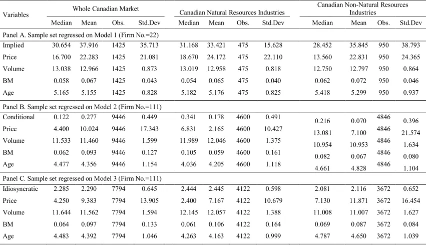
[Please insert Table 1 about here]

Table 1 shows the summary statistics for the sample. Nine subsample periods are looked. The data period is from 2001 to 2014, including 168 months in total. In this 14-year period, both of bull market and bear market are involved. Also, it can be seen that, according to data availability, the sample for Model 1 (Sample data for implied volatility) is limited compared to the other sample sets. Only 22 firms are involved. The sample size for Model 2 is the greatest, including 9446 observations and 111 firms.

Among three measures of volatilities, the average of implied volatility is significantly greater than the other measures of volatilities in all the sample sets. The averages of both of implied volatility and conditional volatility are highest in the Canadian market as a whole while the average of idiosyncratic volatility is highest in the subsample of firms in the natural resource industry. The average firm age is 110 months and it transformed to the natural log value in this study.

4.1.2.1 Conditional Volatility

Conditional volatility is also included and calculated by using E-GARCH model. In this study, one of the statistical tools, E-views, is used to get the results.

The equations of GARCH (1, 1) volatility and E-GARCH (1, 1) are specified as following:

(15)

For the long-run GARCH (1, 1) volatility:

(16)

When it extends to E-GARCH (1, 1) volatility model, the equation will be

(18)

14

The long-run E-GARCH (1, 1) volatility is defined as

(18)

Where:

Guassian distributed innovations/shocks:

GED distributed innovations/shocks:

Student’s t-Distributed innovations/shocks:

is the model’s residual at time t;

is the conditional standard deviation at time t;

From the equations it can be assumed that the conditional volatility might predict the probability of occurrence of extreme volatility in an opposite way as implied and idiosyncratic volatility do, because GARCH models have mean reverting volatility. More specifically, E-GARCH volatilities are always expected to move to the average and this is not the case for the other two measures of volatility. The details of model specifications can better explain Hypothesis 3 in this study.

4.2 Probit Regressions Estimation

To examine the predictive ability of variables, probit regression is chosen in this study. Probit regression is applied in Fodor, Krieger, Mauck, and Stevenson (2013), where the significant relationship is found between options implied volatility and the probability of occurrence of expected extreme returns. Following the methodology in Fodor, Krieger, Mauck, and Stevenson(2013), probit regression is performed to examine how the variables, including implied volatility, conditional volatility, idiosyncratic volatility, firm age, firm price, trading

(19)

15

volume and book-to-market ratio, predict the occurrence of firm extreme return in the next calendar month.

This study regresses the probability of subsequent extreme returns on different volatilities in separate specifications. The specifications of probit regression are shown as following:

Model 1

Model 2

) Model 3

Where is the probability that extreme return occurs, which means . While indicates a non-extreme return observation. To determine extreme returns, the firms that prove to be in the highest or lowest of realized returns in the following period are classified as having extreme returns. In this study, four values are applied, where equals to 1.5, 2.5, 3.5 and 4.5.

represents the cumulative normal distribution function. IV is monthly implied volatility from Canadian option prices collected from Bloomberg. Cond is monthly conditional volatility calculated based on EGARCH model by EVIEWS. Idio is the monthly idiosyncratic volatility measured by using the five-factor model in Fama French (2015) as the standard deviation of regression residuals of each stock in each month. is the natural log of firm age in months, where firm age is calculated based on the initial appearance month in CFMRC. If the initial appearance of any firm is before January 1950, it will be recorded as January 1950. is the book-to-market ratio computed annually based on available data on Compustat, in accordance with equation (12). is the natural log of monthly firm equity price. Vol is the natural log of monthly volume calculated as the average number of shares traded in the previous month (in millions). And is the error term.

The dependent variable represents the probability of extreme returns, and all the explanatory variables are the values in preceding month. The observations of explanatory variables are from the final trading day of preceding month, or over the course of the preceding month. This equation is estimated on a monthly basis and Fama-Macbeth coefficients are calculated using monthly probit

(20)

16

regression coefficients. Also, Newey-West standard errors of monthly coefficients are used to calculate t-statistics.

This study also investigates the relationship for subsamples of firms in Canadian natural resources industry and firms that are not in Canadian natural resources industry. More specifically, each model is performed in three sample sets: the Canadian market as a whole, the subsample of firms in the natural resource industry and subsample of firms in Non-natural resource industry. Additionally, each sample is wished to examine in four different extreme levels. The first level classifies firms that are in the highest 1.5% or lowest 1.5% of realized returns in the following month as having extreme returns. And the other three levels expand the extreme percentage to top 2.5% or bottom 2.5%, top 3.5% or bottom 3.5% and top 4.5% or bottom 4.5%, respectively. However, since the sample size involving implied volatility is limited (only 22 firms are incorporated) the extreme return definition above cannot be applied. Therefore, for sample set involving implied volatility, the firms that ranked as the highest or lowest returns in each month are defined as having extreme returns.

There are two points should be highlighted. First, the daily data are only used to calculate monthly idiosyncratic volatility. To examine the extreme return predictive ability, monthly data are used instead. And there are 168 months in the sample set of this study. Secondly, in the probit regression procedure, a fully ex ante approach is employed to predict extreme returns. All the regressions are conducted based on the probability of extreme returns of the subsequent month and the predictors in this month. In other words, all the variables from a given month are used to predict extreme return status in the following month.

(21)

17

5. Results

5.1 Correlation Matrix for the Predictor Variables

Table 2 displays the correlation matrix for three different sample sets, and the corresponding t-statistics for the predictor variables

As is shown there, price and idiosyncratic volatility is relatively high, which is -0.521. This is to be expected since it has been previously documented in Black and Fischer (1976) that firm’s stock return volatility rise after stock prices fall. The resulting collinearity may tend to weaken the individual impact of these variables to some extent. The other Pearson’s correlation coefficients are quite low (lower than 0.5), showing “weak” or “very weak” correlations.

5.2 Probit Regression Results

The probit regression and the results from Fama-Macbeth procedure are shown below in Table 3 and 4. Newey-West standard errors of monthly coefficients are used to calculate the t-statistics. Three models are regressed in different samples and using different extreme level benchmarks.

Table 3 shows estimates of the Probit model and the Fama Macbeth estimates using implied volatility. As mentioned previously, due to limited data availability, for each month, both of the highest firm return and lowest firm return are defined as extreme returns and no other extreme levels are applied. It can be seen from the table that implied volatility is obviously significant for the Non-natural resources industry, which is consistent with the results of Fodor, Krieger, Mauck, and Stevenson (2013). Here we also show that implied volatility is positively related to the probability of occurrence of expected extreme returns. More specifically, firms with higher implied volatility from option price are 70% more likely to have extreme returns in the subsequent month. However, this relationship is not observed for firms in the natural resource industry or for the entire Canadian market.

(22)

18

For the other variables of firm characteristics, Volume, BM and Age show significantly negative relation with probability of expected extreme returns in Non-natural resource industry. Also, these relations are not significant in natural resource industry.

Table 4 represents probit regression results for Model (2) and Model (3), where Model (2) is regressed for samples incorporating conditional volatility and Model (3) is regressed for samples incorporating idiosyncratic volatility. Different from the sample of Model (1), the sample sizes of these two sets are meaningful to set four different extreme levels. In table 4, Panel A to Panel D represents four different extreme levels, which are top 1.5% and bottom 1.5% of returns (Panel A), top 2.5% and bottom 2.5% of returns (Panel B), top 3.5% and bottom 3.5% of returns (Panel C) and top 4.5% and bottom 4.5% of returns (Panel D).

In Panel A, firms that are in the highest 1.5% or lowest 1.5% of realized returns in the following month are defined as having extreme returns. As is shown, conditional volatility is significantly negatively related to expected extreme returns in all the three sample sets. As the extreme level ranges widen, this relationship disappears. For idiosyncratic volatility, the coefficients are obviously significant in all the extreme levels and sample sets. In another word, firms with extreme returns in following year are more likely to have higher idiosyncratic volatility no matter the firm belongs to natural resource industry or non-natural resource industry. However, the influence of idiosyncratic volatility is less significant in natural resource industry. Compared to conditional volatility and implied volatility, the influence of idiosyncratic volatility for the probability of occurrence of expected extreme returns is more significant and widely applicable.

For the conditional volatility, it is significantly negatively related to the probability of occurrence of extreme returns, but only in Panel A and Panel B. This relationship is different from those of implied volatility and idiosyncratic volatility, which might be explained as that GARCH models have mean reverting volatility, which means their volatility are always expected to move to the average.

For the other explanatory variables, Price is the most significant variable. It is significantly negatively related to the probability of occurrence of expected extreme returns in all extreme

(23)

19

levels and sample sets. Firm age also shows a negative relationship with expected extreme returns. In another word, younger firms and firms with lower stock price are more likely to experience extreme return in the following year. Consistent with the results for Model (1), firms with lower BM are more likely to have extreme returns. However, the coefficients in Model (2) and Model (3) are only significant for whole Canadian market sample and only in Panel B and Panel C. Additionally, BM is never significant in the natural resource industry. For the Volume, the signs of coefficients are mixed and the coefficients are only marginally significant.

6. Conclusion

This study examines the predictive prowess for several factors for predicting extreme returns in the Canadian stock market. Consistent with the results of Fodor, Krieger, Mauck, and Stevenson (2013) for US stocks, implied volatility is positively related to the probability of occurrence of expected extreme returns in the following period. However, for the Canadian market, this relation is only significant in the subsample of firms that are not in the resource sector in Canada or for the Canadian market as a whole. Idiosyncratic volatility, which is calculated by using Fama and French (2015) five-factor model, has the most significant predictive ability among the three measures of volatility. It has a positive coefficient and it is highly significant in a Fama-Macbeth framework in all the sample sets. In another word, no matter whether the firm is in natural resource industry or not, the firms with a high idiosyncratic volatility are more likely to experience extreme returns in the following month. However, we find that the result for the other measure of volatility is in the opposite way. Firms with lower

conditional volatility are more likely to experience extreme return in the next calendar month in

all three samples. Interestingly, this negative relation is only significant when the extreme level return threshold is high. And the reason why that conditional volatility has the negative relationship with expected extreme returns instead of positive might be explained as that GARCH models have mean reverting volatility, which means their volatility are always expected to move to the average. This is not the case for the other two measures of volatility.

(24)

20

This study also finds that younger firms and firms with lower stock price and BM ratio are more likely to experience extreme return in the following year. Trading volume has mixed effects across sectors and for the market as a whole.

Given the importance of predicting extreme returns, it may be worthwhile to expand the analyses to other countries. This remains a topic for future research.

(25)

21

References

Ang, Andrew, Robert J. Hodrick, Yuhang Xing, and Xiaoyan Zhang. "The cross-section of volatility and expected returns." The Journal of Finance 61, no. 1 (2006): 259-299.

An, Li. "Asset Pricing when Traders Sell Extreme Winners and Losers." Available at SSRN 2355520 (2014).

Beneish, Messod D., Lee, Charles MC, and Robin L. Tarpley. "Contextual fundamental analysis through the prediction of extreme returns." Review of Accounting Studies 6.2-3 (2001), 165-189.

Black, Fischer, “Studies of stock price volatility changes,” Proceedings of the 1976 meetings of the American Statistical Association, Business and Economics Statistics Section Washington, DC (1976)l 177-181.

Boehme, Rodney D., Bartley R. Danielsen, Praveen Kumar, and Sorin M. Sorescu. "Idiosyncratic risk and the cross-section of stock returns: Merton (1987) meets Miller (1977)." Journal of Financial Markets 12, no. 3 (2009): 438-468.

Brockman, Paul, and Xuemin Sterling Yan. "Block ownership and firm-specific information." Journal of Banking & Finance 33.2 (2009): 308-316.

Campbell, John Y., Sanford J. Grossman, and Jiang Wang. "Trading volume and serial correlation in stock returns. " No. w4193. National Bureau of Economic

Research, 1992.

Campbell, John Y., Martin Lettau, Burton G. Malkiel, and Yexiao Xu. "Have individual stocks become more volatile? An empirical exploration of idiosyncratic risk." The Journal of Finance 56, no. 1 (2001): 1-43.

(26)

22

Chan, Wing Hong, Ranjini Jha, and Madhu Kalimipalli. "The economic value of using realized volatility in forecasting future implied volatility." Journal of

Financial Research 32, no. 3 (2009): 231-259.

Chen, Nai-Fu, Richard Roll, and Stephen A. Ross. "Economic forces and the stock market." Journal of business (1986): 383-403.

Dong, I., Duan, L. and C. M. J. Jang , “Predicting extreme stock performance more accurately,” Working Paper, (2003) Harvard University.

Doukas, John, and Lorne N. Switzer, “Common Stock Returns and International Listing Announcements: New Tests of the Mild Segmentation Hypothesis,”

Journal of Banking and Finance 24 (March 2000), pp. 471-502

Duffee, Gregory R. "Stock returns and volatility a firm-level analysis." Journal of

Financial Economics 37.3 (1995): 399-420.

Engle, Robert F., David M. Lilien, and Russell P. Robins. "Estimating time varying risk premia in the term structure: The ARCH-M model." Econometrica

(1987) 391-407.

Fama, Eugene F., and Kenneth R. French. "The cross‐section of expected stock returns." Journal of Finance 47.2 (1992), 427-465.

Fama, E. F., and K. R. French, “Common risk factors in the returns on stocks and bonds,”Journal of Financial Economics 25 (1993), 23–49.

(27)

24

Fama, Eugene F., and Kenneth R. French. "A five-factor asset pricing model." Journal of Financial Economics 116.1 (2015): 1-22.

Fink, Jason, Kristin Fink, and Hui He. "Idiosyncratic volatility measures and expected return." Available at SSRN 1692315 (2010).

Fodor, Andy, Krieger, Kevin, Mauck, Nathan, and Greg Peterson (2010). "Predicting Extreme Returns And Portfolio Management Implications." Journal

of Financial Research 36.4 (2013): 471-492.

Frazzini, Andrea, and Lasse Heje Pedersen. "Betting against beta." Journal of

Financial Economics 111.1 (2014): 1-25.

Fu, F. (2009). Idiosyncratic risk and the cross-section of expected stock returns.

Journal of Financial Economics, 91 (1), 24-37.

Fu, F., & Schutte, M. G. “Investor diversification and the pricing of idiosyncratic risk.” Proceedings from the 2010 FMA Asian Conference. Singapore.

Herskovic, Bernard, Bryan Kelly, Hanno Lustig, and Stijn Van Nieuwerburgh. "The common factor in idiosyncratic volatility: Quantitative asset pricing implications." Journal of Financial Economics 119 (2015), 249-283.

Jensen, Michael C., Fischer Black, and Myron S. Scholes. "The capital asset pricing model: Some empirical tests." in Studies in the Theory of Capital Markets,

edited by M. C. Jensen. New York: Praeger, 1972.

L’Her, Jean-François, Tarek Masmoudi, and Jean-Marc Suret. "Evidence to support the four-factor pricing model from the Canadian stock market." Journal

(28)

24

Malkiel, Burton G., and Yexiao Xu. "Idiosyncratic risk and security returns."University of Texas at Dallas (November 2002) (2002).

Mendonça, Fernanda Primo de, Marcelo Cabus Klotzle, Antonio Carlos Figueiredo Pinto, and Roberto Marcos da Silva Montezano. "The relationship between idiosyncratic risk and returns in the Brazilian stock market." Revista

Contabilidade & Finanças 23, no. 60 (2012): 246-257

Merton, Robert C. "A simple model of capital market equilibrium with incomplete information." The journal of finance 42, no. 3 (1987): 483-510.

Merton, Robert C. "An intertemporal capital asset pricing model."Econometrica:

Journal of the Econometric Society (1973): 867-887.

Nelson, Daniel B. “Conditional heteroscedasticity in stock returns: a new approach.” Econometrica 59.2 (1991), 347-370.

Poon, Ser-Huang, and Clive WJ Granger. "Forecasting volatility in financial markets: A review." Journal of Economic Literature 41.2 (2003): 478-539.

Sharpe, William F. "Capital asset prices: A theory of market equilibrium under conditions of risk*." Journal of Finance 19.3 (1964): 425-442.

Spiegel, Matthew I. and Wang, Xiaotong, "Cross-sectional Variation in Stock Returns: Liquidity and Idiosyncratic Risk" (September 8, 2005). Yale ICF Working Paper No. 05-13; EFA 2005 Moscow Meetings Paper. Available at SSRN: http://ssrn.com/abstract=709781.

Switzer, Lorne N., and Alan Picard. "Idiosyncratic Volatility, Momentum, Liquidity, and Expected Stock Returns in Developed and Emerging Markets."

Multinational Finance Journal 19 (2015), 169-221

Switzer, L.N., Lee, Seungho, Zhao, Y. and Zhigang Yang. "Assessing Stock Price Risk in Developed Markets Using Extreme Measures" Concordia University

(29)

25

Appendix

Table 1. Summary Statistics

Variables Whole Canadian Market Canadian Natural Resources Industries

Canadian Non-Natural Resources Industries

Median Mean Obs. Std.Dev Median Mean Obs. Std.Dev Median Mean Obs. Std.Dev Panel A. Sample set regressed on Model 1 (Firm No.=22) Implied 30.654 37.916 1425 35.713 31.168 33.421 475 15.628 28.452 35.845 950 38.793 Price 16.700 22.283 1425 21.081 18.670 24.172 475 22.110 13.560 22.831 950 24.365 Volume 13.038 12.966 1425 0.873 13.019 12.958 475 0.818 12.750 12.797 950 0.864 BM 0.058 0.067 1425 0.043 0.054 0.065 475 0.040 0.062 0.072 950 0.046 Age 5.165 5.155 1425 0.828 5.182 5.176 475 0.825 5.418 5.299 950 0.937 Panel B. Sample set regressed on Model 2 (Firm No.=111) Conditional 0.122 0.277 9446 0.449 0.341 0.178 4600 0.491 _0.216 _0.070 4846 _0.396 Price 4.400 10.024 9446 17.343 6.831 2.165 4600 10.427 _13.081 _7.100 4846 _21.574 Volume 11.533 11.460 9446 1.599 11.989 12.046 4600 1.375 10.954 10.953 4846 1.634 BM 0.062 0.093 9446 0.127 0.105 0.059 4600 0.161 _0.082 _0.067 4846 _0.080 Age 4.477 4.356 9446 1.154 4.036 4.205 4600 1.118 4.661 4.828 4846 1.104 Panel C. Sample set regressed on Model 3 (Firm No.=111) Idiosyncratic 2.285 2.290 7794 0.645 2.444 2.445 4122 0.598 2.081 2.116 3672 0.652 Price 4.250 9.383 7794 13.905 2.400 7.167 4122 10.679 7.130 11.871 3672 16.454 Volume 11.644 11.562 7794 1.594 12.145 12.057 4122 1.388 11.008 11.007 3672 1.627 BM 0.064 0.097 7794 0.133 0.061 0.106 4122 0.164 0.069 0.087 3672 0.084 Age 4.483 4.392 7794 1.046 4.263 4.163 4122 0.999 4.787 4.650 3672 1.039

(30)

26

Table 2. Correlation Matrix

Sample Set (1) Implied Price Volume BM Age

Implied 1 Price -0.271*** 1 (-10.62) Volume 0.007 0.292*** 1 (0.25) (11.51) BM 0.217*** -0.309*** -0.168*** 1 (8.4) (-12.28) (-6.45) Age -0.079*** 0.271*** 0.306*** -0.025 1 (-2.98) (10.64) (12.14) (-0.95)

Sample Set (2) Conditional Price Volume BM Age

Conditional 1 Price -0.262*** 1 (-26.53) Volume -0.072*** 0.139*** 1 (-7.04) (13.70) BM 0.274*** -0.169*** -0.041*** 1 (27.75) (-16.69) (-3.96) Age -0.087*** 0.176*** 0.096*** -0.025** 1 (-8.49) (17.44) (9.39) (-2.47) (Continued)

(31)

27

Table 2. Continued.

Sample Set (3) Idiosyncratic Price Volume BM Age

Idiosyncratic 1 Price -0.521*** 1 (-53.93) Volume -0.028** 0.233*** 1 (-2.44) (21.13) BM 0.238*** -0.185*** -0.038*** 1 (-21.64) (-16.67) (-3.36) Age -0.183*** 0.246*** 0.130*** -0.049*** 1 (-16.46) (22.37) (11.55) (-4.38)

Note: This table shows the correlation matrix among five variables in three different sample sets. Sample Set (1) includes data that will be regressed on Model (1); Sample Set (2) includes data that will be regressed on Model (2); Sample Set (3) includes data that will be regressed on Model (3); Implied is the monthly implied volatility collected form Bloomberg. Conditional is the monthly conditional volatility calculated by EGARCH model. Idiosyncratic is the monthly idiosyncratic volatility calculated by five-factor model introduced in Fama and French (2015). Price is the natural log of firm price. Volume is the natural log of the monthly volume calculated as the average number of shares traded in the previous month (in millions). BM is the book-to-market ratio. Size is the log of firm size (in millions of dollars). Age is the natural log of firm age in months. All observations are collected and computed based on available data from 2001 to 2014 and must have data for all measures.

***Significant at the 1% level **Significant at the 5% level *Significant at the 10% level

(32)

28

Table 3. Probit Regression Results for Implied Volatility

Whole Market Natural Resources Non-Natural Resources

Model 1 Model 1 Model 1

Implied 0.29 0.03 0.7*** (0.6) (0.14) (3.16) Price -0.27 0.03 -0.04 (-0.49) (0.2) (-0.46) Volume -2.81 -3.57 -3.77* (-0.24) (-0.94) (-1.71) BM -226.21*** -8.47 -173.52*** (-2.63) (-0.14) (-3.91) Age -8.61 1.87 -4.87*** (-0.69) (0.62) (-3.26) No. of Observations 1425 475 950 No. of Extremes 230 117 220 No. of Firms 22 8 14

Note: This table shows regression results for Model (1). 22 firms in total are involved. This table presents coefficients and t-statistics of the Fama-Macbeth procedure. The extreme returns in each month are defined as the biggest and the smallest firm returns. Probit regressions of the likelihood of a firm having extreme stock returns in the following year are involved in this procedure. Different sample set are regressed, respectively. And the results are shown in three different columns. Implied is the monthly implied volatility from Canadian option price collected form Bloomberg. Price is the firm price. Volume is the log of the monthly volume calculated as the average number of shares traded in the previous month (in millions). BM is the book-to-market ratio. Age is the firm age in months. All observations are collected and computed based on available data from 2001 to 2014 and must have data for all measures.

***Significant at the 1% level **Significant at the 5% level. *Significant at the 10% level.

(33)

29

Table 4. Probit Regression Results for Conditional & Idiosyncratic Volatility

Whole Market Natural Resources Non-Natural Resources Model 2 Model 3 Model 2 Model 3 Model 2 Model 3 Panel A: Top 1.5% and Bottom 1.5% of returns

Cond. -4.32** -8.45** -4.92** (-1.68) (-2.59) (-2.17) Idio. 2.64*** 2.84** 2.01** (2.78) 2.15 2.17 Price -0.79*** -0.59*** -1.00*** -0.614*** -0.49*** -0.41*** (-6.18) (-4.62) (-5.44) (-3.6) (-6.31) (-4.78) Volume 0.29 0.56 0.47 -0.068 0.18 0.18 (1.43) (1.44) (1.1) (-0.1) (0.53) (0.7) BM -9.80 -2.79 10.54 -7.047 -17.01* -9.00 (-1.2) -0.41 (1.09) (-0.67) (-1.67) (-0.6) Age -0.41 -0.57* -0.01 -0.79 0.17 -0.03 (-1.28) (-1.76) (-0.01) (-1.34) (0.32) (-0.06) No. of Observations 9483 7794 4638 4122 4845 3672 No. of Extremes 289 187 160 143 158 146 No. of Firms 111 111 62 62 49 49

Panel B: Top 2.5% and Bottom 2.5% of returns

Cond. -0.57 -7.32** -4.84** (-0.57) (-2.35) (-2.06) Idio. 2.42*** 2.53* 1.95** (3.81) (1.95) (2.17) Price -0.58*** -0.67*** -0.96*** -0.63*** -0.53*** -0.39*** (-5.72) (-5.9) (-5.35) (-3.55) (-5.24) (-4.81) Volume 0.28** 0.15 0.38 -0.019 0.09 0.21 (1.69) (0.61) (0.95) (-0.03) (0.23) (0.84) BM 0.41 -2.11 12.26 -4.914 -11.86 -9.91 (0.08) (-0.34) (1.32) (-0.48) (-1.19) (-0.68) Age -0.46** -0.79*** -0.03 -0.98* 0.53 -0.03 (-1.69) (-2.68) (-0.06) (-1.69) (0.8) (-0.06) No. of Observations 9483 7794 4638 4122 4845 3672 No. of Extremes 440 359 196 158 174 156 No. of Firms 111 111 62 62 49 49

(34)

30 Table 4. Continued

Panel C: Top 3.5% and Bottom 3.5% of returns

Cond. 1.37 -0.89 -3.35 (1.55) (-0.29) (-1.22) Idio. 1.49*** 1.63* 2.21** (2.92) (1.97) (2.48) Price -0.28*** -0.58*** -0.88*** -0.67*** -0.52 -0.38*** (-4.69) (-4.67) (-5.22) (-5.05) (-4.92***) (-4.58) Volume 0.37 _(1.4) _(-0.87)-0.09 _(0.99)0.35 _(0.45)0.18 _(-0.66)-0.25 _(0.73)0.19 BM -9.65** -6.09* 14.17 7.16 -12.74 -10.88 (-1.96) (-1.77) (1.61) (0.74) (-1.15) (-0.77) Age -0.02 -0.18 -0.14 -1.11* 0.48 0.15 (-0.2) (-0.7) (0.39) (-1.83) (0.64) (0.26) No. of Observations 9483 7794 4638 4122 4845 3672 No. of extremes 709 590 365 332 394 213 No. of Firms 111 111 62 62 49 49

Panel D: Top 4.5% and Bottom 4.5% of returns

Cond. 1.34 -1.97 -2.63 (1.62) (-0.65) (-0.94) Idio. 1.14** 2.28** 2.31** (2.49) (2.28) (2.56) Price -0.21*** -0.39*** -1.03*** -0.75*** -0.63*** -0.49*** (-4.54) -4.64 (-5.62) -4.29 (-5.57) (-5.46) Volume 0.34 -0.07 0.28 -7.32 -0.58* 0.52* (1.28) (-0.73) (0.9) (-0.53) (-1.69) (1.77) BM -10.06** -6.44* 12.89 25.05 -17.06 -17.88 (-2.14) (-1.95) (1.45) (1.02) (-1.38) (-1.19) Age -0.04 -0.1 -0.26 -1.51** 1.00 0.03 (-0.45) (-0.45) (-0.8) (-2.41) (1.34) (0.06) No. of Observations 9483 7794 4638 4122 4845 3672 No. of extremes 868 689 402 393 488 366 No. of Firms 111 111 62 62 49 49

Note: This table shows regression results for Model (2) and Model (3). This table presents coefficients, t-statistics and P-Value of the Fama-Macbeth procedure. Probit regressions of the likelihood of a firm having extreme stock returns in the following year are involved in this procedure. Different sample set are regressed, respectively. And the results are shown in three different columns. Different thresholds of “extreme” are showed specifically and the numbers of predicted extreme returns in different groups are presented in this table. Conditional is the monthly conditional volatility calculated through EGARCH. Idiosyncratic is the monthly idiosyncratic volatility calculated by five-factor model introduced in Fama and French (2015). Price is the firm price. Volume is the log of the monthly volume calculated as the average number of shares traded in the previous month (in millions).

BM is the book-to-market ratio. Age is the firm age in months. All observations are collected and computed based on available data from 2001 to 2014 and must have data for all measure

(35)

Predicting Extreme Returns in the Canadian Stock Market