Pricing Bermudan options under local Lévy models with default

Contents lists available atScienceDirect

Journal

of

Mathematical

Analysis

and

Applications

www.elsevier.com/locate/jmaa

Pricing

Bermudan

options

under

local

Lévy

models

with

default

A. Borovykha, A. Pascuccia,∗, C.W. Oosterleeb,c

a

DipartimentodiMatematica,UniversitàdiBologna,Bologna,Italy b

CentrumWiskunde&Informatica,Amsterdam,TheNetherlands c_{DelftUniversityofTechnology,Delft,TheNetherlands}

a r t i cl e i n f o a b s t r a c t

Articlehistory:

Received27April2016

Availableonline27January2017 SubmittedbyH.-M.Yin

Keywords:

Bermudanoption LocalLévymodel Defaultableasset Asymptoticexpansion Fourier-cosineexpansion

Weconsideradefaultableassetwhoserisk-neutralpricingdynamicsaredescribed by an exponential Lévy-type martingale.This class of models allowsfor a local volatility,localdefaultintensityandalocallydependentLévymeasure.Wepresent apricingmethodforBermudanoptionsbasedonananalyticalapproximationofthe characteristicfunctioncombinedwiththeCOS method.Due toa specialformof theobtainedcharacteristicfunctionthepricecanbecomputedusingafastFourier transform-basedalgorithmresultinginafastandaccuratecalculation.TheGreeks canbecomputedatalmostnoadditionalcomputationalcost.Errorboundsforthe approximationofthecharacteristicfunctionaswellasforthetotaloptionpriceare given.

©2017ElsevierInc.Allrightsreserved.

1. Introduction

Infinancialmathematics,thefastandaccuratepricingoffinancialderivativesisanimportantbranchof research.Dependingonthetypeoffinancialderivative,themathematicaltaskisessentiallythecomputation ofintegrals,andthissometimesneedstobeperformedinarecursivewayinatime-wisedirection.Formany stochasticprocessesthatmodelthefinancialassets,theseintegralscanbe mostefficientlycomputedinthe Fourierdomain.However,forsomerelevantandrecentstochasticmodelstheFourierdomaincomputations are notatall straightforward,as these computations relyontheavailability ofthecharacteristic function ofthestochasticprocess (read:theFouriertransformofthetransitionalprobabilitydistribution),whichis not known. This is especially true for state-dependent asset price processes, and for asset processes that includethenotion ofdefault intheirdefinition. Withthederivations and techniques inthepresent paper wemakeavailablethehighlyefficientpricingofso-calledBermudanoptionstotheabovementionedclasses of state-dependent asset dynamics, including jumps inasset pricesand the possibility of default. In this

* Correspondingauthor.

E-mailaddresses:[email protected](A. Borovykh),[email protected](A. Pascucci),[email protected]

(C.W. Oosterlee).

http://dx.doi.org/10.1016/j.jmaa.2017.01.071

sense,theclassofassetmodels forwhichFourieroptionpricingishighly efficientincreasesbythecontents of thepresentpaper. Essentially,we approximatethecharacteristicfunctionby anadvancedTaylor-based expansioninsuchawaythattheresultingcharacteristicfunctionexhibitsfavorablepropertiesforthepricing methods.

Fouriermethodshaveoftenbeenamong thewinners inoptionpricingcompetitionssuchasBENCHOP

[16]. In [5], aFourier method called the COS method, as introduced in [4], was extended to the pricing of Bermudanoptions.Thecomputationalefficiencyofthemethodwasbasedonaspecific structureofthe characteristic function allowing to use the fast Fourier transform (FFT) for calculating the continuation valueoftheoption.Fouriermethodscanreadilybeappliedtosolvingproblemsunderassetpricedynamics for whichthecharacteristic functionisavailable.ThisisthecaseforexponentialLévymodels,suchasthe Merton model developed in [13], the Variance-Gamma model developed in [12], but also for the Heston model [6].However, inthecase oflocal volatility, default and state-dependent jump measures there isno closed formcharacteristic functionavailableandtheCOSmethodcannot be readilyapplied.

Recently,in[14]theso-calledadjointexpansionmethod fortheapproximationofthecharacteristic func-tion inlocal Lévymodels ispresented. Thismethodisworked outintheFourierspacebyconsideringthe adjointformulationofthepricingproblem,thatisusingabackwardparametrixexpansionaswasalsolater donein[1].Inthispaperwegeneralizethismethodtoincludeadefaultableassetwhoserisk-neutralpricing dynamics aredescribed byanexponential Lévy-typemartingalewithastate-dependent jumpmeasure,as hasalsobeen consideredin[11]andin[7].

Having obtained theanalytical approximation forthe characteristic functionwe combine thiswith the COSmethodforBermudanoptions.Weshowthatthisanalyticalformulaforthecharacteristicfunctionstill possessesastructurethatallowstheuseofaFFT-basedmethodinordertocalculatethecontinuationvalue. ThisresultsinanefficientandaccuratecomputationoftheBermudanoptionvalueandoftheGreeks.The characteristic function approximationused intheCOS methodisalready veryaccurate forthe 2nd-order approximation, meaning that the explicit formulas are simple and this makes methodeasy and quick to implement.Weproveerrorboundsforthe0th- and1st-orderapproximation,justifyingtheaccuracyofthe methodandpresentawiderangeofnumericalexamples,showing theflexibility,accuracyandspeedofthe method.

2. Generalframework

Weconsider adefaultableassetS whoserisk-neutraldynamicsaregiven by:

St=1{t<ζ}eXt, dXt=μ(t, Xt)dt+σ(t, Xt)dWt+ R dN˜t(t, Xt−, dz)z, dN˜t(t, Xt−, dz) =dNt(t, Xt−, dz)−ν(t, Xt−, dz)dt, ζ= inf{t≥0 : t 0 γ(s, Xs)ds≥ε}, (2.1)

where N˜t(t,x,dz) is acompensated random measure with state-dependent Lévy measure ν(t,x,dz). The

default time ζ of S is defined ina canonical way as the first arrival time of a doubly stochastic Poisson process withlocalintensity functionγ(t,x)≥0,andε∼Exp(1) andisindependent ofX.Thus themodel features:

• alocalvolatility functionσ(t,x);

• alocal Lévymeasure:jumpsinX arrivewith astate-dependent intensity described bythelocal Lévy measure ν(t,x,dz).Thejumpintensityandjumpdistributioncanthuschangedependingonthevalue ofx.Astate-dependentLévymeasureisanimportantfeaturebecauseitallowstoincorporatestochastic jump-intensity intothemodelingframework;

• alocaldefault intensityγ(t,x):theassetS candefault withastate-dependentdefaultintensity.

Thiswayofmodelingdefaultisalsoconsideredinadiffusivesettingin[3]andforexponential Lévymodels in[2].

WedefinethefiltrationofthemarketobservertobeG=FX_{∨ F}D_,whereFX _{isthefiltrationgenerated}

byX and FD

t :=σ({ζ≤u},u≤t),fort≥0,isthefiltrationofthedefault.Weassume

R

e|z|ν(t, x, dz)<∞,

and by imposing that the discounted asset price S˜t := e−rtSt is a G-martingale, we get the following

restrictiononthedriftcoefficient:

μ(t, x) =γ(t, x) +r−σ 2_{(t, x)} 2 − R ν(t, x, dz)(ez−1−z).

Isitwell-known(see,forinstance,[8,Section2.2])thatthepriceV ofaEuropeanoptionwithmaturityT

andpayoffΦ(ST) isgivenby

Vt=1{ζ>t}e−r(T−t)E e−tTγ(s,Xs)ds_φ(X T)|Xt , t≤T, (2.2) where φ(x)= Φ(ex_{). Thus,inorder to computethe priceof anoption,we must evaluatefunctionsof the}

form u(t, x) :=E e−tTγ(s,Xs)dsφ(X_T)|X_t=x . (2.3)

Understandardassumptions,ucanbe expressedastheclassicalsolutionofthefollowingCauchyproblem

Lu(t, x) = 0, t∈[0, T[, x∈R, u(T, x) =φ(x), x∈R,

whereL istheintegro-differentialoperator

Lu(t, x) =∂tu(t, x) +r∂xu(t, x) +γ(t, x)(∂xu(t, x)−u(t, x)) + σ2_{(t, x)} 2 (∂xx−∂x)u(t, x) − R ν(t, x, dz)(ez−1−z)∂xu(t, x) + R ν(t, x, dz)(u(t, x+z)−u(t, x)−z∂xu(t, x)). (2.4)

Thefunctionuin(2.3) canbe representedasanintegralwith respectto thetransitiondistributionof the defaultablelog-priceprocesslogS:

u(t, x) =

R

Here we notice explicitly that Γ(t,x;T,dy) is notnecessarily a standard probability measure because its integral overRcanbe strictly lessthan one;nevertheless,with aslightabuseof notation,we saythatits Fouriertransform ˆ Γ(t, x;T, ξ) :=F(Γ(t, x;T,·))(ξ) := R eiξyΓ(t, x;T, dy), ξ∈R,

is thecharacteristic functionof logS.

2.1. Adjointexpansionof thecharacteristicfunction

In this section we generalize the results in [14] to our framework and develop an expansion of the coefficients

a(t, x) := σ

2_{(t, x)}

2 , γ(t, x), ν(t, x, dz),

around somepointx¯.Thecoefficients a(t,x),γ(t,x) andν(t,x,dz) are assumedto be continuously differ-entiable withrespectto xuptoorderN ∈N.

From nowonforsimplicityweassumethatthecoefficientsareindependentoft(seeRemark 2.2forthe generalcase).Firstweintroducethenth-order approximationofLin(2.4):

Ln=L0+ n k=1 (x−x¯)kak(∂xx−∂x) + (x−x¯)kγk∂x−(x−x¯)kγk − R (x−x¯)kνk(dz)(ez−1−z)∂x+ R (x−x¯)kνk(dz)(ez∂x−1−z∂x) , where L0=∂t+r∂x+a0(∂xx−∂x) +γ0∂x−γ0− R ν0(dz)(ez−1−z)∂x+ R ν0(dz)(ez∂x−1−z∂x), and ak= ∂xka(¯x) k! , γk= ∂xkγ(¯x) k! , νk(dz) = ∂xkν(¯x, dz) k! , k≥0.

Thebasepointx¯isaconstantparameterwhichcanbechosenfreely.Ingeneralthesimplestchoiceisx¯=x

(thevalue oftheunderlyingat initialtime t): wewill seethatinthiscase theformulasfortheBermudan optionvaluation aresimplified.

Let us assume for a moment that L0 has a fundamental solution G0(t,x;T,y) that is defined as the

solutionoftheCauchyproblem

L0G0(t, x;T, y) = 0 t∈[0, T[, x∈R,

G0_{(T,·;T, y) =δ}

y.

Inthis casewedefine thenth-orderapproximationofΓ as

Γ(n)(t, x;T, y) =

n

k=0

where,foranyk≥1 and(T,y),Gk_{(·,·;T,y) isdefinedrecursivelythroughthefollowing Cauchyproblem} ⎧ ⎪ ⎨ ⎪ ⎩ L0Gk(t, x;T, y) =− k h=1 (Lh−Lh−1)Gk−h(t, x;T, y) t∈[0, T[, x∈R, Gk_{(T, x;T, y) = 0, x∈R.} Noticethat Lh−Lh−1= (x−x¯)hah(∂xx−∂x) + (x−x¯)hγh∂x−(x−x¯)hγh − R (x−x¯)hνh(dz)(ez−1−z)∂x+ R (x−x¯)hνh(dz)(ez∂x−1−z∂x).

Correspondingly,thenth-order approximationofthecharacteristicfunctionΓ isˆ definedtobe

ˆ Γ(n)(t, x;T, ξ) = n k=0 FGk(t, x;T,·)(ξ) := n k=0 ˆ Gk(t, x;T, ξ), ξ∈R. (2.6) Now weremark thatthe operatorLacts on(t,x) whilethecharacteristic functionis aFourier transform takenwith respect toy: inorderto takeadvantageof suchatransformation,inthefollowing theorem we characterizeˆΓ(n)_{intermsoftheFouriertransformoftheadjointoperatorL}˜_{= ˜L}(T ,y)_{ofL,actingon(T,y).}

Theorem2.1(Dual formulation).Forany(t,x)∈]0,T]×R,thefunctionG0(t,x;·,·) isdefinedthroughthe followingdual Cauchyproblem

˜ L(₀T ,y)G0_{(t, x;T, y) = 0 T > t, y∈R,} G0(T, x;T,·) =δx, (2.7) where ˜ L(₀T ,y)=−∂T −r∂y+a0(∂yy+∂y)−γ0∂y−γ0+ R ν0(dz)(ez−1−z)∂y+ R ¯ ν0(dz)(ez∂y −1−z∂y).

Moreover, foranyk≥1,thefunctionGk_{(t,x;·,·) isdefinedthroughthedual Cauchyproblem asfollows:}

⎧ ⎪ ⎨ ⎪ ⎩ ˜ L(₀T ,y)Gk_{(t, x;T, y) =−}k h=1 ˜ L_h(T ,y)−L˜(_hT ,y₋₁) Gk−h_{(t, x;T, y) T > t, y∈R,} Gk_{(T, x;T, y) = 0 y∈R,} (2.8) with ˜ L(_hT ,y)−L˜(_hT ,y₋₁)=ahh(h−1)(y−x¯)h−2+ah(y−x¯)h−1(2h∂y+ (y−x¯)(∂yy+∂y) +h) −γhh(y−x¯)h−1−γh(y−x¯)h(∂y+ 1) + R νh(dz)(ez−1−z) h(y−x¯)h−1+ (y−x¯)h∂y + R ¯ νh(dz) (y+z−x¯)hez∂y −_(y−_x¯)h−_zh(y−_x¯)h−1−_(y−_x¯)h_∂ y ,

where indefining theadjointof theoperatorweusethenotation ez∂y_{f(y) :=} ∞ n=0 zn n!∂ n yf(y) =f(y+z).

Notice thattheadjointCauchyproblems(2.7)and (2.8)admitasolutionintheFourierspaceand canbe solved explicitly;infact,wehave

F_L˜(T ,·) 0 G

k_{(t, x;T,·) (ξ) =ψ(ξ) ˆG}k_{(t, x;T, ξ)−∂}

TGˆk(t, x;T, ξ),

where ψ(ξ) isthecharacteristicexponentoftheLévyprocesswithcoefficientsγ0,a0andν0(dz),thatis

ψ(ξ) =iξ(r+γ0) +a0(−ξ2−iξ)−γ0− R ν0(dz)(ez−1−z)iξ+ R ν0(dz)(eizξ−1−izξ).

Thus thesolution(intheFourierspace)to problems(2.7)and(2.8)isgivenby

ˆ G0(t, x;T, ξ) =eiξx+(T−t)ψ(ξ), ˆ Gk(t, x;T, ξ) =− T t eψ(ξ)(T−s)F _k h=1 ˜ L(_hs,·)−L˜_h(s,₋·₁) Gk−h(t, x;s,·) (ξ)ds, k≥1. (2.9)

Now we considerthe generalframeworkand inparticularwe dropthe assumptionon theexistenceofthe fundamentalsolutionofL0:inthiscase,wedefinethenth-orderapproximationofthecharacteristicfunction

ˆ

Γ asin(2.6),withGˆk givenby(2.9).Wealsonoticethat

F_L˜(s,·) h −L˜ (s,·) h−1 u(s,·) (ξ) = ahh(h−1)(−i∂ξ−x¯)h−2+ah(−i∂ξ−x¯)h−1

−2hiξ+ (−i∂ξ−x¯)(−ξ2−iξ) +h

ˆ

u(s, ξ)

−γhh(−i∂ξ−x¯)h−1−γh(−i∂ξ−x¯)h(iξ−1)

ˆ u(s, ξ) + R νh(dz)(ez−1−z)

h(−i∂ξ−x¯)h−1−(−i∂ξ−x¯)hiξ

ˆ u(s, ξ) + R νh(dz)

(−i∂y−z−x¯)heiξz−(−i∂y−x¯)h+z

h(−i∂ξ−x¯)h−1−(−i∂ξ−x¯)hiξ

ˆ

u(s, ξ).

Remark 2.2. In case the coefficients γ, σ, ν depend on time, the solutions to the Cauchy problems are similar: ˆ G0(t, x;T, ξ) =eiξxetTψ(s,ξ)ds, ˆ Gk(t, x;T, ξ) =− T t esTψ(τ,ξ)dτF _k h=1 ˜ L(_hs,·)(s)−L˜_h(s,₋·₁)(s) Gk−h(t, x;s,·) (ξ)ds, with

ψ(s, ξ) =iξ(r+γ0(s)) +a0(s)(−ξ2−iξ)− R ν0(s, dz)(ez−1−z)iξ+ R ν0(s, dz)(eizξ−1−izξ), ˜ L(_hs,y)(s)−L˜(_hs,y₋₁)(s) =ah(s)h(h−1)(y−x¯)h−2+ah(s)(y−x¯)h−1(2h∂y+ (y−x¯)(∂yy+∂y) +h) −γh(s)h(y−x¯)h−1−γh(s)(y−x¯)h(∂y+ 1) + R νh(s, dz)(ez−1−z) h(y−x¯)h−1+ (y−x¯)h∂y + R ¯ νh(s, dz) (y+z−x¯)hez∂y −_(y−_x¯)h−_zh(y−_x¯)h−1−_(y−_x¯)h_∂ y .

From these results onecanalready see thatthe dependencyon xcomes inthrough eiξx _{and after taking}

derivativesthedependencyonxwilltaketheform (x−x¯)m_eiξx_{:thisfactwillbe crucialinouranalysis.}

Example2.3.Toseetheabovedependencymoreexplicitlyforthesecond-orderapproximationofthe char-acteristicfunctionweconsider,foreaseofnotation,asimplifiedmodel:aone-dimensionallocalLévymodel wherethelog-pricesolvestheSDE

dXt=μ(Xt)dt+σ(Xt)dWt+

R

dN˜t(dz)z. (2.10)

This modelisasimplificationoftheoriginal model,sincewe consideronly alocalvolatility function,and no local default or state-dependent Lévy measure. Thus only a Taylor expansion of the local volatility coefficientisused.However,thedependencythatwewillseegeneralizesinthesamewaytothelocaldefault andstate-dependent measure.Bythemartingaleconditionwe have

μ(x) =r−a(x)−

R

ν(dz)(ez−1),

andthereforetheKolmogorovoperatorof (2.10)reads

Lu(t, x) =∂tu(t, x) +r∂xu(t, x) +a(t, x)(∂xx−∂x)u(t, x) − R ν(dz)(ez−1) + R ν(dz) (u(t, x+z)−u(t, x)).

In this case, we have the following explicit approximation formulas for the characteristic function ˆ Γ(t,x;T,ξ): ˆ Γ(t, x;T, ξ) ≈ Γˆ(n)(t, x;T, ξ) :=eiξx+(T−t)ψ(ξ) n k=0 ˆ Fk(t, x;T, ξ), n≥0, (2.11) with ψ(ξ) =irξ−a0(ξ2+iξ)− R ν(dz)(ez−1)iξ+ R ν(dz)eizξ−1, and ˆ Fk(t, x;T, ξ) = k h=0 g_h(k)(T−t, ξ)(x−x¯)h; (2.12)

here,fork= 0,1,2,we have g₀(0)(s, ξ) = 1, g₀(1)(s, ξ) =a1s2(ξ2+iξ) i 2ψ _(ξ), g₁(1)(s, ξ) =−a1s(ξ2+iξ), g₀(2)(s, ξ) = 1 2s 2_a 2ξ(i+ξ)ψ(ξ)− 1 6s 3_ξ(i+ξ)(a2 1(i+ 2ξ)ψ(ξ)−2a2ψ(ξ)2+a21ξ(i+ξ)ψ(ξ)) −1 8s 4_a2 1ξ2(i+ξ)2ψ(ξ)2, g₁(2)(s, ξ) = 1 2s 2_ξ(i+ξ)(a2 1(1−2iξ) + 2ia2ψ(ξ))− 1 2s 3_ia2 1ξ2(i+ξ)2ψ(ξ), g₂(2)(s, ξ) =−a2sξ(i+ξ) + 1 2s 2_a2 1ξ2(i+ξ)2.

Usingthenotationfromabove,wecanwriteinthesamewaytheapproximationformulasforthegeneral case. Here wepresent theresults fork= 0,1,sincehigher-order formulas aretoo longto include.Forthe full formulawerefertoAppendix B.Wehave:

g(0)₀ (s, ξ) =1, g(1)₀ (s, ξ) =i 2a1s 2_(ξ2_{+iξ)ψ(ξ) +}1 2γ1s 2_{(i+ξ)ψ(ξ)−}1 2 R ν1(dz)(ez−1−z)s2ξψ(ξ) (2.13) −1 2 R ν1(dz)(ieiξz−i+ξz)s2ψ(ξ), g(1)₁ (s, ξ) =−a1s(ξ2+iξ) +γ1si(i+ξ)− R ν1(dz)(ez−1−z)sξi + R ν1(dz)(eiξz−1−ξiz)s.

Remark2.4. From(2.11)–(2.12)weclearlyseethattheapproximationofordernisafunctionoftheform

ˆ Γ(n)(t, x;T, ξ) :=eiξx n k=0 (x−x¯)kgn,k(t, T, ξ), (2.14)

where the coefficientsgn,k, with0≤k≤n, dependonly ont,T andξ,butnot onx.The approximation

formulacanthusalwaysbesplitintoasumofproductsoffunctionsdependingonlyonξandfunctionsthat are linearcombinations of(x−x¯)m_eiξx_,m∈N

0.

3. Bermudanoptionvaluation

ABermudanoptionisafinancialcontractinwhichtheholdercanexerciseatapredeterminedfinitesetof exercisemomentspriortomaturity,andtheholderoftheoptionreceivesapayoffwhenexercising.Consider aBermudanoptionwithaset ofM exercisemoments{t1,...,tM},with0≤t1< t2<· · ·< tM =T.When

theoptionisexercisedattimetmtheholderreceivesthepayoffΦ(tm, Stm).Recalling(2.2),theno-arbitrage

v(t, Xt) =1{ζ>t} sup τ∈Tt Ee−tτ(r+γ(s,Xs))ds_{φ(τ, X} τ)|Xt , where φ(t,x) = Φ(t,ex_{) and T}

t is the set of all G-stopping times taking values in {t1,...,tM}∩[t,T].

For a Bermudan put option with strike price K, we simply have φ(t,x) = (K−ex₎+

. By the dynamic programmingapproach,theoptionvaluecanbe computedbyabackwardrecursion:wedenoteby

˜

v(tM, x) =φ(tM, x), v(tM, x) =1{ζ>tM}φ(tM, x),

thepre-defaultvalueandthetruevalueof thepayoff respectively;moreover,weset ⎧ ⎨ ⎩ ˜ c(t, x) =Ee−ttm(r+γ(s,Xs))dsv˜(t_m, X_t m)|Xt=x , t∈[tm−1, tm[ ˜ v(tm−1, x) = max{φ(tm−1, x),c˜(tm−1, x)}, m∈ {2, . . . , M}. (3.15)

Intheabovenotation˜c(t,x) istheso-calledpre-defaultcontinuationvalue:the“true”continuationvalueis givenby c(t, x) =1_{ζ>t}c˜(t, x) =E e−r(tm−t)₁ {ζ>tm}˜v(tm, Xtm)|Gt .

Theoptionvalueisdefinedas

v(t, m) =

1_{ζ>tm−1}v˜(tm−1, x), fort=tm−1,

c(t, m), fort∈]tm−1, tm[, and, ift1>0, also fort∈[0, t1[.

Wenoticeexplicitlythatthepricingalgorithm (3.15)requires,ateachstep,toevaluateexplicitlyonlythe

pre-default continuation value: this makes the algorithm feasible since the item 1_{ζ>t} cannot be priced

explicitly.

Remark3.5. Sincethepayoffofacalloptiongrowsexponentiallywiththelog-stockprice,thismayintroduce significant cancelation errors for large domain sizes. For this reason we price putoptions only using our approach and weemploy the well-knownput-call parity to price calls viaputs. This is arather standard argument(see,forinstance,[17]).

3.1. Analgorithm forpricingBermudan putoptions

The COS method proposed by [5] is based on the insight thatthe Fourier-cosine series coefficients of Γ(t,x;T,dy) (and therefore also of option prices) are closely related to the characteristic function of the underlyingprocess,namelythefollowingrelationshipholds:

b a eibkπ−aΓ(t, x;T, dy)≈ˆΓ t, x;T, kπ b−a .

TheCOSmethodprovides away tocalculatingexpectedvalues(integrals)oftheform

v(t, x) =

R

φ(T, y)Γ(t, x;T, dy),

1. Inthefirststepwetruncatetheinfiniteintegrationrangeto [a,b] toobtainapproximationv1: v1(t, x) := b a φ(T, y)Γ(t, x;T, dy).

Weassumethiscanbe doneduetotherapiddecayofthedistributionatinfinity. 2. Inthesecondstepwereplacethedistributionwith itscosine expansionand weget

v1(t, x) := b−a 2 ∞ k=0 Ak(t, x;T)Vk(T),

where indicatesthatthefirstterminthesummationisweightedbyone-half and

Ak(t, x;T) = 2 b−a b a cos kπy−a b−a Γ(t, x;T, dy), Vk(T) = 2 b−a b a cos kπy−a b−a φ(T, y)dy,

aretheFourier-cosine seriescoefficientsofthedistributionandofthepayofffunctionattimeT respec-tively.DuetotherapiddecayoftheFourier-cosineseriescoefficients,wetruncatetheseriessummation andobtainapproximationv2:

v2(t, x) := b−a 2 N−1 k=0 Ak(t, x;T)Vk(T).

3. Inthethirdstepweuse thefactthatthe coefficientsAk canbe rewrittenusing thetruncated

charac-teristicfunction: Ak(t, x;T) = 2 b−aRe ⎛ ⎝e−ikπb−aa b a eibkπ−ayΓ(t, x;T, dy) ⎞ ⎠.

Thefiniteintegrationrangecanbeapproximatedas

b a eibkπ−ay_{Γ(t, x;T, dy)}≈ R eibkπ−ay_{Γ(t, x;T, dy) = ˆΓ} t, x;T, kπ b−a .

Thusinthelast stepwe replaceAk byitsapproximation:

2 b−aRe e−ikπb−aaΓˆ t, x;T, kπ b−a ,

andobtainapproximationv3:

v3(t, x) := N−1 k=0 Re e−ikπb−aaˆ_Γ t, x;T, kπ b−a Vk(T). (3.16)

NextwegobacktotheBermudanputpricingproblem.Rememberingthattheexpectedvaluec(t,x) in

(3.15)canberewritteninintegralformasin(2.5),wehave

c(t, x) =e−r(tm−t)

R

v(tm, y)Γ(t, x;tm, dy), t∈[tm−1, tm[.

ThenweusetheFourier-cosineexpansion(3.16),so thatwegettheapproximation:

ˆ c(t, x) =e−r(tm−t) N−1 k=0 Re e−ikπb−aa_Γˆ t, x;tm, kπ b−a Vk(tm), t∈[tm−1, tm[ (3.17) Vk(tm) = 2 b−a b a cos kπy−a b−a max{φ(tm, y), c(tm, y)}dy, withφ(t,x)= (K−ex)+.

Nextwe recover thecoefficients(Vk(tm))k=0,1,...,N−1 from (Vk(tm+1))k=0,1,...,N−1. To thisend,we split

theintegralinthedefinitionofVk(tm) intotwoparts usingtheearly-exercisepointx∗m,whichisthepoint

wherethecontinuationvalueisequalto thepayoff,i.e.c(tm,x∗m)=φ(tm,x∗m);thuswehave

Vk(tm) =Fk(tm, x∗m) +Ck(tm, x∗m), m=M−1, M−2, ...,1, where Fk(tm, x∗m) := 2 b−a x∗m a φ(tm, y) cos kπy−a b−a dy, Ck(tm, x∗m) := 2 b−a b x∗_m c(tm, y) cos kπy−a b−a dy, (3.18) andVk(tM)=Fk(tM,logK).

Remark 3.6. Since we have a semi-analytic formula for cˆ(tm,x), we can easily find the derivatives with

respect to x and use Newton’s method to find the point x∗m such that c(tm,x∗m) = φ(tm,x∗m). A good

startingpointfortheNewtonmethodislogK,sincex∗_m≤logK.

ThecoefficientsFk(tm,x∗m) canbe computedanalyticallyusingx∗m≤logK,sothatwehave Fk(tm, x∗m) = 2 b−a x∗m a (K−ey) cos kπy−a b−a dy = 2 b−aKΨk(a, x ∗ m)− 2 b−aχk(a, x ∗ m), where χk(a, x∗m) = x∗m a eycos kπy−a b−a dy = 1 1 + kπ b−a 2 ex∗m_cos kπx ∗ m−a b−a −ea+kπe x∗m b−a sin kπx ∗ m−a b−a ,

1. Fork= 0,1, ..., N−1:

•At timetM, the coefficients are exact:Vk(tM) =Fk(tM,logK), as in(3.18).

2. Form=M−1 to 1:

•Determine the early-exercise pointx∗musing Newton’s method;

•Compute ˆVk(tm) using formula ˆVk(tm) :=Fk(tm, x∗m) + ˆCk(tm, x∗m),(3.18)and(3.19). Use an FFT for the continuation

value (see Section3.2).

3. Final step: using ˆVk(t1) determine the option price ˆv(0, x) = ˆc(0, x) using(3.17). Fig. 1.Algorithm3.1: Bermudan option valuation.

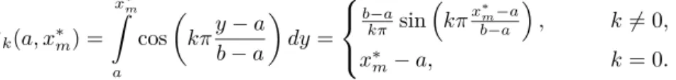
Ψk(a, x∗m) = x∗_m a cos kπy−a b−a dy= ⎧ ⎨ ⎩ b−a kπ sin kπx∗m−a b−a , k= 0, x∗_m−a, k= 0.

On the other hand,by inserting theapproximation (3.17) for thecontinuation valueinto theformula for

Ck(tm,x∗m) havethefollowingcoefficientsCˆk form=M−1,M−2,...,1:

ˆ Ck(tm, x∗m) = 2e−r(tm+1−tm) b−a N−1 j=0 Vj(tm+1) b x∗ m Re e−ijπb−aaΓˆ tm, x;tm+1, jπ b−a cos kπx−a b−a dx. (3.19)

Thus thealgorithm forpricingBermudanoptionscanthenbesummarized asinFig. 1.

3.2. Anefficientalgorithm forthecontinuationvalue

InthissectionwederiveanefficientalgorithmforcalculatingCˆk(tm,x∗m) in(3.19).Whenconsideringan

exponential Lévyprocess withconstantcoefficientsasdonein[5],thecontinuationvaluecanbecalculated using aFast Fourier Transform(FFT). This can be done due to the factthat thecharacteristic function ˆ

Γ(t,x;T,ξ) canbe split intoaproduct ofafunction dependingonlyon ξand afunction oftheform eiξx_.

Notethatwetypicallyhaveξ=_bjπ_−a.TheintegrationoverxresultsinasumofaHankelandToeplitzmatrix (withindices(j+k) and(j−k) respectively).Thematrix-vectorproduct,withthesespecialmatrices,can be transformedintoacircularconvolution whichcanbecomputed usingFFTs.

From (2.14)weknowthatthenth-orderapproximationofthecharacteristic functionisoftheform:

ˆ Γ(n)(tm, x;tm+1, ξ) =eiξx n k=0 (x−x¯)kgn,k(tm, tm+1, ξ),

where the coefficientsgn,k(t,T,ξ), with 0≤k≤n, depend onlyont,T andξ,butnoton x. Using (2.14)

we writethecontinuationvalueas:

ˆ Ck(tm, x∗m) = n h=0 e−r(tm+1−tm) N−1 j=0 Re Vj(tm)gn,h tm, tm+1, jπ b−a M_k,jh (x∗_m, b) ,

where wehaveinterchangedthesumsandintegraland defined:

M_k,jh (x∗_m, b) = 2 b−a b x∗m eijπxb−−aa_(x−_x¯)h_cos kπx−a b−a dx. (3.20)

Thiscanbewritteninvectorizedform as: ˆ C(tm, x∗m) = n h=0 e−r(tm+1−tm)_ReV(t m+1)Mh(x∗m, b)Λh ,

whereV(tm+1) isthevector[V0(tm+1),...,VN−1(tm+1)]T andMh(x∗m,b)Λhisamatrix-matrixproductwith

Mh _{beingamatrixwithelements{M}h

k,j}Nk,j−=01 andΛh isadiagonalmatrixwithelements

gn,h

tm, tm+1,

jπ

b−a , j = 0, . . . , N−1.

Wehavethefollowing theoremfor calculatingageneralizedform oftheintegralin(3.20)whichisused in thecalculationofthecontinuationvalue.

Theorem3.7. The matrixMwith elements{Mk,j}Nk,j−=01 suchthat:

Mk,j =

ejxcos(kx)xmdx,

consists ofsumsof HankelandToeplitzmatrices.

Proof. Using standardtrigonometric identitieswecanrewritetheintegralas:

Mk,j = cos(jx) cos(kx)xmdx+i sin(jx) cos(kx)xmdx =M_k,jH +iM_k,jT ,

wherewe havedefined:

M_k,jH =1 2 cos((j+k)x)xmdx+1 2 sin((j+k)x)xmdx, M_k,jT =1 2 cos((j−k)x)xmdx+1 2 sin((j−k)x)xmdx.

Thefollowingholds: cos(nx)xmdx=1 nx m_{sin(nx) +} m/2 i=1 (−1)i+1 2i−2 j=0(m−j) n2i cos(nx)x m−(2i−1) − m/2 i=1 (−1)i+1 2i−1 j=0 (m−j) n2i+1 sin(nx)x m−2i_, sin(nx)xmdx=− 1 nx m_{cos(nx) +} m/2 i=1 (−1)i+1 2i−2 j=0(m−j) n2i sin(nx)x m−(2i−1) − m/2 i=1 (−1)i+1 2i−1 j=0 (m−j) n2i+1 cos(nx)x m−2i_.

Itfollowsthat{M_k,jH}_k,jN−₌₀1 isaHankelmatrixwithcoefficient(j+k) and{M_k,jT }_k,jN−₌₀1 isaToeplitz matrix withcoefficient(j−k):

MH = ⎛ ⎜ ⎜ ⎜ ⎜ ⎝ M0 M1 M2 . . . MN−1 M1 M2 . . . MN .. . ... MN−2 MN−1 . . . M2N−3 MN−1 . . . M2N−3 M2N−2 ⎞ ⎟ ⎟ ⎟ ⎟ ⎠, MT = ⎛ ⎜ ⎜ ⎜ ⎜ ⎝ M0 M1 . . . MN−2 MN−1 M₋1 M0 M1 . . . MN−2 .. . . .. ... M2−N . . . M−1 M0 M1 M1−N M2−N M−1 M0 ⎞ ⎟ ⎟ ⎟ ⎟ ⎠, where wehavedefined

Mj = 1 2 cos(jx)xmdx+1 2 sin(jx)xmdx. 2

FromTheorem 3.7weseethatMh_(x∗

m,b) withelementsMk,jh consistsofasumofaHankelandToeplitz

matrix.

Example3.8.WederiveexplicitlytheHankelandToeplitzmatricesform= 0 andm= 1.Wecalculatethe indefiniteintegral Mk,j= 2 b−a eijπxb−−aa_cos kπx−a b−a (x−x¯)mdx.

Supposem= 0,inthiscasewehaveMk,j =Mk,jH +Mk,jT ,with:

M_k,jH =− iexpi(j+k_b)₋π(_ax−a) π(j+k) , Mk,jT =− iexpi(j−k_b)₋π(_ax−a) π(j−k) ,

where {M_k,jH}N_k,j−₌₀1 isaHankel matrixand {M_k,jT }N_k,j−₌₀1 isaToeplitzmatrixwith

Mj = ⎧ ⎨ ⎩ x b−a, j= 0, −iexp ijπ_b(x₋−_aa) πj , j= 0.

Supposem= 1,inthiscasewehave:

M_k,jH =− a−b (j−k)2_π2exp i(j−k)π(x−a) b−a − x−x¯ (j−k)πiexp i(j−k)π(x−a) b−a , M_k,jT =− a−b (j+k)2_π2exp i(j+k)π(x−a) b−a − x−x¯ (j+k)πiexp i(j+k)π(x−a) b−a ,

where {M_k,jH}N_k,j−₌₀1 isaHankel matrixand {M_k,jT }N_k,j−₌₀1 isaToeplitzmatrix,with

Mj = ⎧ ⎨ ⎩ x(x−x¯) b−a , j= 0, −a−b j2_π2exp ijπ(x_b−_−aa) −x−x¯ jπ iexp ijπ(x_b−−_aa) , j= 0.

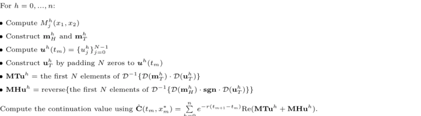
1. Forh= 0, ..., n: •ComputeMh j(x1, x2) •ConstructmhH andm h T •Computeuh_(t m) ={uhj} N−1 j=0

•ConstructuhT by paddingNzeros tou h

(tm)

•MTuh_{= the firstNelements ofD}−1_{D(mh T)· D(u

h T)}

•MHuh= reverse{the firstNelements ofD−1{D(mhH)·sgn· D(u h T)}}

2. Compute the continuation value using ˆC(tm, x∗m) = n

h=0

e−r(tm+1−tm)_Re(MTuh_+MHuh_).

Fig. 2.Algorithm3.2: Computation of ˆC(tm, x∗m).

Remark3.9.If wetakex¯=x, whichis mostcommoninpractice,theformulas aresimplifiedsignificantly andonlythecaseofm= 0 isrelevant.Inthiscasethecharacteristicfunctionissimplyeiξx_timesasumof

termsdependingonlyontm, tm+1 andξ= _bjπ_−a:

ˆ

Γ(n)(tm, x;tm+1, ξ) =eiξxgn,0(tm, tm+1, ξ).

UsingthesplitintosumsofHankelandToeplitz matriceswecanwritethecontinuationvalueinmatrix form as: ˆ C(tm, x∗m) = n h=0 e−r(tm+1−tm)_Re(Mh H+MhT)uh ,

where Mh_H ={M_k,jH,h(x∗m,b)}Nk,j−=01 isaHankel matrix andMlT ={M T ,h k,j (x∗m,b)}k,jN−=01 is aToeplitz matrix anduh_={uh j}Nj=0−1,with uhj =gn,h tm, tm+1,_bjπ_−a Vj(tm+1) anduh0 = 12gn,h(tm, tm+1,0)V0(tm+1).

We recall that the circular convolution, denoted by , of two vectors is equal to the inverse discrete Fouriertransform(D−1_{) oftheproductsoftheforwardDFTs,D,i.e.:}

xy=D−1{D(x)· D(y)}.

ForHankeland Toeplitzmatriceswehavethefollowingresult:

Theorem3.10. ForaToeplitzmatrix MT,theproduct MTuisequal tothefirstN elements ofmT uT,

wheremT anduT are 2N vectors definedby

mT = [M0, M−1, M−2, ..., M1−N,0, MN−1, MN−2, ..., M1]T, uT = [u0, u1, ..., uN−1,0, ...,0]T.

ForaHankelmatrixMH,theproductMHuisequaltothefirstN elementsof mHuHinreversedorder,

wheremH anduH are2N vectorsdefined by

mH = [M2N−1, M2N−2, ..., M1, M0]T uH = [0, ...,0, u0, u1, ..., uN−1]T.

Summarizing,wecancalculatethecontinuationvalueCˆ(tm,x∗m) usingthealgorithminFig. 2.

ThecontinuationvaluerequiresfiveDFTsforeachh= 0,...,n,andaDFTiscalculatedusingtheFFT. In practiceit is most common to havex¯= xand inthis casewe only need fiveFFTs. The computation

of Fk(tm,x∗m) is linear in N. The overall complexity of the method is dominated by the computation of

ˆ

C(tm,x∗m),whose complexity is O(Nlog2N) with the FFT.Thecomplexity ofthe calculation foroption

valueat time0isO(N). IfwehaveaBermudanoptionwith M exercisedates, theoverallcomplexity will be O((M−1)Nlog₂N).

Remark3.11(Americanoptions).ThepricesofAmericanoptionscanbeobtainedbyapplyingaRichardson extrapolation(see,forinstance,[9])onthepricesofafewBermudanoptionswithasmallnumberofexercise dates. Let vM denote thevalue ofaBermudanoptionwith maturityT and anumberM of earlyexercise

datesthatare _MT yearsapart.Then,foranyd∈N,thefollowing4-pointRichardsonextrapolationscheme 1

21(64v2d+3−56v2d+2+ 14v2d+1−v2d) givesanapproximationofthecorresponding Americanoptionprice.

Remark3.12(TheGreeks). TheapproximationmethodcanalsobeusedtocalculatetheGreeksatalmost no additional cost. In the case of ¯x = x, we have the following approximation formulas for Delta and Gamma: ˆ Δ =e−r(t1−t0) N−1 k=0 Re eikπxb−−aa ikπ b−agn,0 t0, t1, kπ b−a +gn,1 t0, t1, kπ b−a ˆ Vk(t1), ˆ Γ =e−r(t1−t0) N−1 k=0 Re eikπxb−−aa − ikπ b−agn,0 t0, t1, kπ b−a −gn,1 t0, t1, kπ b−a + 2 ikπ b−agn,1 t0, t1, kπ b−a + ikπ b−a 2 gn,0 t0, t1, kπ b−a + 2gn,2 t0, t1, kπ b−a Vˆk(t1). 4. Errorestimates

The error in our approximation consists of the error of the COS method and the error inthe adjoint expansion of the characteristic function. The errorof the COS methoddepends on the truncation of the integration range[a,b] andthetruncation oftheinfinitesummationof theFourier-cosine expansionbyN. Thedensityrapidlydecaystozeroasy→ ±∞.Then theoverallerrorcanbeboundedas follows:

1(x;N,[a, b])≤Q R\[a,b] Γ(t, x;T, dy) + P (N−1)β−1 ,

where P andQareconstantsnotdependingonN or[a,b] andβ≥n≥1,withnbeingthealgebraicindex of convergenceofthecosine seriescoefficients.For asufficiently largeintegration interval[a,b],theoverall errorisdominatedbytheseriestruncationerror,whichconvergesexponentially.Theerrorinthebackward propagation of the coefficients Vk(tm) is defined as 2(k,tm) := Vk(tm)−Vˆk(tm). With [a,b] sufficiently

largeandaprobabilitydensityfunctioninC∞([a,b]),theerror1(k,tm) convergesexponentiallyinN.For

adetailedderivationontheerroroftheCOSmethodsee[4]and[5].

Wenowpresenttheerrorestimatesfortheadjointexpansionofthecharacteristicfunctionatorderszero and one.Weconsider forsimplicityamodelwithtime-independentcoefficients

Xt=x+ t 0 μ(Xs)ds+ t 0 σ(Xs)dWs+ t 0 R η(Xs−)zdN˜(s, dz), (4.21)

where we have defined as usual dN˜(t,dz) = dN(t,dz)−ν(dz)dt. This model is similar to the model we consideredinitiallyin(2.1);onlynowwedealwithslightlysimplifiedversionandassumethatthedependency onXt inthemeasurecanbefactoredout,whichisoftenenoughthecase.

LetX˜t bethe0th-orderapproximationofthemodelin(4.21)withx¯=x, thatis

˜ Xt=x+ t 0 μ(x)ds+ t 0 σ(x)dWs+ t 0 R η(x)zdN˜(s, dz). (4.22)

ThecharacteristicexponentofX˜t−xis

ψ(ξ) =iξμ(x)−σ(x) 2 2 ξ 2_−η(x) R ν(dz)(ez−1−z)iξ+η(x) R ν(dz)(eizξ−1−izξ). (4.23)

Theorem 4.13. Let n = 0,1 and assume that the coefficients μ,σ,η are continuously differentiable with bounded derivatives upto order n. Let Γˆ(n)_{(0,x;t,ξ) in (2.6) be the nth-order approximation of the}

char-acteristic function. Then,for any T >0 thereexists apositiveconstant C that depends onlyon T,on the normsof thecoefficientsandon theLévymeasureν,such that

_Γ(0ˆ _{, x;t, ξ)−}ˆ_Γ(n)_{(0, x;t, ξ)≤C1 +|ξ|}1+3n_tn+1_{, t∈[0, T], ξ∈R. (4.24)}

Proof. FortheproofwerefertoAppendix A. 2

Remark4.14.TheproofofTheorem 4.13canbegeneralizedtoobtainerrorboundsforanyn∈N:however, onecanseethat, forn≥2,theorder of convergenceimprovesonly inthediffusivepart,accordingto the resultsprovedin[10].

5. Numericalexperiments

In this section we apply the method developedin Section4 to compute the European and Bermudan optionvalueswithvariousunderlyingstockdynamics.ThecomputerusedintheexperimentshasanIntel Corei7CPUwitha2.2GHzprocessor.Weusethesecond-orderapproximationofthecharacteristicfunction. We have found this to be sufficiently accurate by numerical experiments and theoretical error estimates. Theformulasforthesecond-orderapproximation aresimple,makingthemethodeasytoimplement.

FortheCOSmethod,unlessotherwisementioned,weuseN = 200 andL= 10,whereListheparameter usedto definethetruncationrange[a,b] as follows:

[a, b] := c1−L c2+√c4, c1+L c2+√c4 ,

where cn is the nth cumulantof log-price process logS, as proposed in[4]. Thecumulants are calculated

using the0th-orderapproximationof thecharacteristicfunction. AlargerN andL haslittleeffecton the price,sinceafastconvergenceisachievedalreadyforsmallN andL.Wecomparetheapproximatedvalues to a 95% confidenceinterval computed with a Longstaff–Schwartz method with 105 _{simulations and 250}

Table 1

PricesforaEuropeanandaBermudanputoption(expiryT= 0.25 with3exercisedates,expiryT = 1 with10exercisedatesand expiryT = 2 with20exercisedates)intheCEV-Mertonmodelforthe2nd-orderapproximationofthecharacteristicfunction, andaMonteCarlomethod.

T K European Bermudan

MC 95% c.i. Value MC 95% c.i. Value 0.25 0.6 0.001240–0.001433 0.001326 0.001243–0.001431 0.001307 0.8 0.005218–0.005679 0.005493 0.005314–0.005774 0.005421 1 0.04222–0.04321 0.04275 0.04274–0.04371 0.04304 1.2 0.1923–0.1938 0.1935 0.1979–0.1989 0.1981 1.4 0.3856–0.3872 0.3866 0.3948–0.3958 0.3955 1.6 0.5812–0.5829 0.5825 0.5940–0.5950 0.5941 1 0.6 0.006136–0.006573 0.006579 0.006307–0.006729 0.006096 0.8 0.02526–0.02622 0.02581 0.02617–0.02711 0.02520 1 0.08225–0.08395 0.08250 0.08480–0.08640 0.08593 1.2 0.1965–0.1989 0.1977 0.2097–0.2115 0.2132 1.4 0.3560–0.3589 0.3574 0.3946–0.3957 0.3954 1.6 0.5341–0.5385 0.5364 0.5930–0.5941 0.5932 2 0.6 0.01444–0.01513 0.01529 0.01528–0.01594 0.01365 0.8 0.04522–0.04655 0.04613 0.04596–0.04719 0.04659 1 0.1046–0.1067 0.1077 0.1149–0.1168 0.1171 1.2 0.2054–0.2083 0.2065 0.2319–0.2341 0.2345 1.4 0.3351–0.3386 0.3382 0.3968–0.3987 0.3991 1.6 0.4904–0.4944 0.4919 0.5927–0.5938 0.5935

5.1. Testsunder CEV-Mertondynamics

ConsideraprocessundertheCEV-Merton dynamics:

dXt= r−a(Xt)−λ em+δ2/2−1 dt+ 2a(Xt)dWt+ R dN˜t(t, dz)z, with a(x) = σ 2 0e2(β−1)x 2 , ν(dz) =λ√ 1 2πδ2exp −(z−m)2 2δ2 dz,

ψ(ξ) =−a0(ξ2+iξ) +irξ−iλ

em+δ2/2−1 ξ+λemiξ−δ2ξ2/2−1 .

We usethefollowing parametersS0= 1, r= 5%,σ0= 20%, β = 0.5,λ= 30%, m=−10%,δ= 40% and

computetheEuropeanand Bermudanoptionvalues.

We present the results in Table 1. The option value for both the Bermudan options as well as the European options appearsto be accurate. Since the COS method has a very quick convergence, already for N = 64 the errorbecomesstable. Forat-the-money strikeswe havelog₁₀|error| ≈3.5.The useof the second-orderapproximationofthecharacteristicfunctionisjustifiedbythefactthattheoptionvalue(and thustheerror)stabilizesstartingfromthesecond-orderapproximation.Furthermore,itisnoteworthythat the 0th-order approximation is already very accurate. The CPU time of thecalculations depends on the number ofexercisedates. Assumingwe usethesecond-orderapproximation ofthe characteristicfunction, ifwehaveM exercisedatestheCPUtimewillbe 5·M ms.

Remark5.15.Themethodcanbeextendedtoincludetime-dependentcoefficients.Theaccuracyandspeed of themethodwillbe ofthesameorder asfortime-independentcoefficients.

Table 2

Prices foraEuropeanandaBermudan putoption (10exercisedates,expiryT = 1)inthe CEV-VGmodel forthe2nd-order approximationofthecharacteristicfunction,andaMonteCarlomethod.

K European Bermudan

MC 95% c.i. Value MC 95% c.i. Value

0.6 0.03090–0.03732 0.03546 0.03756–0.03876 0.03749 0.8 0.08046–0.08247 0.08029 0.08290–0.08484 0.08395 1 0.1507–0.1531 0.1511 0.1572–0.1600 0.1594 1.2 0.2501–0.2538 0.2522 0.2634–0.2668 0.2685 1.4 0.3831–0.3876 0.3847 0.4073–0.4108 0.4137 1.6 0.5430–0.5479 0.5436 0.5920–0.5938 0.5937

Remark5.16.The Greekscan be calculated at almost noadditional cost using theformulas presented in

3.12. Numerically, the order of convergence is algebraic and is the samefor both the exactcharacteristic functionasforthe2nd-order approximation.

5.2. Testsunder theCEV-Variance-Gammadynamics

Considerthejumpprocess tobe aVariance-Gammaprocess. TheVGprocess, isobtainedbyreplacing thetime inaBrownianmotion withdriftθ andstandarddeviation ,by aGamma processwith variance

κandunitary mean.Themodelparametersand κallowto controltheskewnessand thekurtosisof the distributionofstockpricereturns.TheVGdensityischaracterizedbyafattailandisthususedasamodel insituationswheresmallandlargeassetvaluesaremoreprobablethanwouldbethecaseforthelognormal distribution.TheLévymeasureinthiscaseisgivenby:

ν(dx) = e −λ1x κx 1{x>0}dx+ eλ2x κ|x|1{x<0}dx, where λ1= ! θ2_κ2 4 + 2_κ 2 + θκ 2 −1 , λ2= ! θ2_κ2 4 + 2_κ 2 − θκ 2 −1 . Furthermorewehave a(x) = σ 2 0e2(β−1)x 2 , μ(t, x) =r+1 κlog 1−κθ−κ 2 2 −a(x), ψ(ξ) =−a0(ξ2+iξ) +irξ+i 1 κlog 1−κθ−κ 2 2 ξ−1 κlog 1−iκθξ+ξ 2_κ2 2 .

We use thefollowing parametersS0 = 1,r = 5%, σ0 = 20%, β = 0.5, κ= 1, θ =−50%, = 20%. The

resultsfortheEuropeanandBermudanoptionarepresented inTable 2.

5.3. Testsunder aCEV-likeLévyprocess with astate-dependentmeasureanddefault

Inthissectionweconsideramodelsimilartotheoneusedin[7].Themodelisdefinedwithlocalvolatility, localdefault andastate-dependentLévymeasureas follows:

a(x) =1 2(b

2

Table 3

PricesforaEuropeanandaBermudanputoption(10exercisedates,expiryT = 1)intheCEV-likemodelwithstate-dependent measureforthe2nd-orderapproximationcharacteristicfunction,andaMonteCarlomethod.

K European Bermudan

MC 95% c.i. Value MC 95% c.i. Value

0.8 0.01025–0.01086 0.009385 0.01068–0.01125 0.01024 1 0.04625–0.04745 0.04817 0.05141–0.05253 0.05488 1.2 0.1563–0.1582 0.1564 0.1942–0.1952 0.1952 1.4 0.3313–0.3334 0.3314 0.3927–0.3934 0.3930 1.6 0.5207–0.5229 0.5218 0.5919–0.5926 0.5920 1.8 0.7103–0.7124 0.7122 0.7906–0.7913 0.7910 Table 4

Prices foraEuropeanandaBermudanputoption(10exercisedates,expiryT = 1)intheCEV-likemodelwithdefaultforthe 2nd-orderapproximationcharacteristicfunction,andaMonteCarlomethod.

K European Bermudan

MC 95% c.i. Value MC 95% c.i. Value

0.8 0.002905–0.003175 0.003061 0.005876–0.006245 0.006361 1 0.01845–0.01918 0.01893 0.03419–0.03506 0.03520 1.2 0.08148–0.08296 0.08297 0.1820–0.1827 0.1824 1.4 0.2184–0.2205 0.2173 0.3793–0.3801 0.3792 1.6 0.3867–0.3892 0.3841 0.5752–0.5763 0.5763 1.8 0.5597–0.5638 0.5556 0.7727–0.7739 0.7733 γ(x) =c0+2c1η(x), ν(x, dz) =3νN(dz) +4η(x)νN(dz), η(x) =eβx. (5.25)

Wewill considerGaussian jumps,meaningthat

νN(dz) =λ 1 √ 2πδ2exp −(z−m)2 2δ2 dz.

TheregularCEVmodelhasseveralshortcomings;forinstance,thevolatilitydropstozeroastheunderlying approaches infinity; also the model does not allow the underlying to experience jumps. This model tries to overcome these shortcomings, whilestill retaining CEV-likebehavior through η(x). Thelocal volatility function σ(x) behaves asymptotically like theCEV model, σ(x)∼ √1b1eβx/2 as x→ −∞,reflecting the

fact that the volatility tends to increase as the asset price drops (the leverage effect). Jumps of size dz

arrivewithastate-dependentintensityofν(x,dz).Lastly,adefaultarriveswithintensityγ(x).Thedefault function γ(x) behaves asymptotically like 2c1eβx as x → −∞, reflecting the fact thata default is more

likelytooccur whenthepricegoesdown.

In Table 3 the results are presented for a model as defined in (5.25) without default, meaning that

c0=c1= 0 andwithastate-dependent jumpmeasure,soν(x,dz)=η(x)νN(dz).Inthiscasewehave

ψ(ξ) =irξ−a0(ξ2−iξ)−λν0(em+δ

2_/2

−1)iξ+λν0(emiξ−δ

2_ξ2_/2

−1),

wherea0=1₂b21eβ¯xandν0(dz)=eβx¯νN(dz).Theotherparametersarechosenas:b1= 0.15,b0= 0,β =−2,

λ = 20%, δ = 20%, m =−0.2,S0 = 1, r = 5%,1 = 1, 3 = 0, 4 = 1, the numberof exercise dates is

10 and T = 1.From the resultsfor both the European optionand the Bermudan optionwe see thatthe methodperformsveryaccurately,evenfordeeplyin-the-moneystrikes.

InTable 4theresultsarepresented forthevalueofadefaultableputoption.Incaseofdefault priorto exercisetheputoptionpayoffis 0,incaseofno defaultthevalueis (K−St)+,dependingontheexercise

time.Welookatthemodelasdefinedin(5.25)withthepossibilityofdefaultandconsiderstate-independent jumps,meaningthatwe haveγ(x)=η(x) andν(x,dz)=νN(dz).Wehave

ψ(ξ) =irξ−a0(ξ2−iξ) +γ0iξ−γ0−λ(em+δ

2

/2_{−1)iξ+λ(e}miξ−δ2ξ2/2_−1),

where a0= 1₂b21eβx¯ andγ0=c1eβx¯.Theother parametersareb0= 0, b1= 0.15, β=−2,c0= 0,c1= 0.1,

S0= 1, r= 5%,1= 1,2= 1,3= 1,4= 0,thenumberof exercisedatesis10and T= 1.

Acknowledgments

Wethankananonymousrefereeforsomecommentsthatimprovedthepaper.

Appendix A. ProofofTheorem 4.13

LetX and X˜ be asin(4.21)and(4.22)respectively.Wefirstprovethat

E[|Xt−X˜t|2]≤C

κ2t2+κ21t3

, t∈[0, T], (A.1) for somepositive constantC that depends onlyon T, onthe Lipschitz constants of the coefficientsμ, σ,

η and onthe Lévymeasure ν. Here κ1 =−ψ(0) andκ2=−ψ(0) where ψ in(4.23)is thecharacteristic

exponentoftheLévyprocess ( ˜Xt−x).

UsingtheHölderinequality,theItôisometry(see,forinstance,[15])andtheLipschitzcontinuityofη,μ

andσ,themeansquarederrorisboundedby:

E"|Xt−X˜t|2 # ≤3E ⎡ ⎢ ⎣ ⎛ ⎝ t 0 (μ(Xs)−μ(x))ds ⎞ ⎠ 2⎤ ⎥ ⎦+ 3E ⎡ ⎢ ⎣ ⎛ ⎝ t 0 (σ(Xs)−σ(x))dWs ⎞ ⎠ 2⎤ ⎥ ⎦ + 3E ⎡ ⎢ ⎣ ⎛ ⎝ t 0 R (η(Xs−)−η(x))zdN˜(s, dz) ⎞ ⎠ 2⎤ ⎥ ⎦ ≤C t 0 E"|X˜s−x|2 # ds+C t 0 E"|Xs−X˜s|2 # ds, (A.2) where C= 6 ⎛ ⎝μ2_∞+σ2_∞+η2_∞ R z2ν(dz) ⎞ ⎠.

Nowwerecallthefollowing relationshipbetweenthefirstandsecond momentandcumulants

E[( ˜Xs−x)] =c1(s), E[( ˜Xs−x)2] =c2(s) +c1(s)2, where cn(s) = s in ∂n_ψ(ξ) ∂ξn ξ=0 ,

and ψ(ξ) isthecharacteristicexponentof( ˜Xs−x).Thuswehave E"|X˜s−x|2

#

=κ2s+κ21s2. (A.3)

Plugging(A.3)into(A.2)weget

E[|Xt−X˜t|2]≤C κ2 2t 2₊κ21 3t 3 +C t 0 E"|Xs−X˜s|2 # ds,

and thereforeestimate(A.1)follows byapplying theGronwallinequalityintheform

φ(t)≤α(t) +C t 0 φ(s)ds =⇒ φ(t)≤α(t) +C t 0 α(s)eC(t−s)ds,

thatisvalidforany C≥0 andφ,αcontinuousfunctions. From (A.1)and (A.3)wecanalsodeducethat

E|Xt−x|2 ≤2EXt−X˜t 2 + 2EX˜t−x 2 ≤Cκ2t+κ21t2 , t∈[0, T]. (A.4) Moreover, from (A.1) we also get the following error estimate for the expectation of a Lipschitz payoff functionv:

E[v(Xt)]−E[v( ˜Xt)]≤C

κ2t+κ21t2, t∈[0, T],

where now C also depends on the Lipschitz constantof v. In particular, taking v(x) = eixξ_{, this proves}

(4.24) forn= 0.

Nextweprove(4.24)forn= 1.

Proceeding asintheproofofLemma6.23in[10]withu(0,x)= ˆΓ(0,x;t,ξ) andx¯=x,wefind

ˆ Γ(0, x;t, ξ)−Γˆ(1)(0, x;t, ξ) = t 0 E(L−L0) ˆG1(s, Xs;t, ξ) + (L−L1) ˆG0(s, Xs;t, ξ) ds,

where the1st-orderapproximationisas usual ˆ Γ(1)(s, X;t, ξ) = ˆG0(s, X;t, ξ) + ˆG1(s, X;t, ξ), with ˆ G0(s, X;t, ξ) =eiXξ+(t−s)ψ(ξ), ˆ G1(s, X;t, ξ) =eiXξ+(t−s)ψ(ξ)g(1)₀ (t−s, ξ),

and g(1)₀ as in(2.13).UsingtheLagrangianremainderof theTaylor expansion,wehave

L−L0=γ(ε)(X−x)(∂X−1) +a(ε)(X−x)(∂XX −∂X) +η(ε)(X−x) R ν(dz)(ez−1−z)∂X +η(ε)(X−x) R ν(dz)(ez∂X−₁−_z∂ X),

L−L1= 1 2γ _(ε)(X−x)2_(∂ X−1) + 1 2a _(ε)(X−x)2_(∂ XX −∂X) +1 2η _(ε)(X−x)2 R ν(dz)(ez−1−z)∂X+ 1 2η _(ε)(X−x)2 R ν(dz)(ez∂X −₁−_z∂ X),

forsomeε,ε∈[x,X]. Now,|Gˆ0|≤1 becauseGˆ0isthecharacteristicfunctionoftheprocessX˜ in(4.22); thus,wehave

(L−L1) ˆG0(s, Xs;t, ξ)≤C(1 +|ξ|2)|Xs−x|2.

Ontheotherhand,from(2.13) wehave

g(1)₀ (t−s, ξ)≤C(t−s)21 +|ξ|4,

andthereforeweget (L−L0) ˆG1(s, Xs;t, ξ)≤C(t−s)2(1 +|ξ|4)|Xs−x|. Sowefind _Γ(0ˆ _{, x;t, ξ)−Γ}ˆ(1)_{(0, x;t, ξ)≤C(1 +|ξ|}4₎ t 0 (t−s)2E[|Xs−x|] +E |Xs−x|2 ds

Thethesisthenfollowsfrom estimate(A.4)andintegrating.

Appendix B. The2nd-orderapproximationofthe characteristicfunction

Forcompletenesswepresentheretheformulasofthecharacteristicfunctionapproximationinthegeneral case upto the 2nd-order approximation fora process as in (2.1)with a local-volatilitycoefficient a(t,x), a localdefaultintensityγ(t,x) andastate-dependentmeasureν(t,x,dz).Weexpandthecoefficientsaround ¯

x=x.This choiceofx¯ismostcommoninpracticeanditsimplifiestheformulassignificantly.Wehave

ˆ G(0)(t, x;T, ξ) =eiξx+(T−t)ψ(ξ) ˆ G(1)(t, x;T, ξ) = ˆG(0)(t, x;T, ξ) 1 2i(T −t) 2_ξ(i+ξ)α 1ψ(ξ) + 1 2(T−t) 2_(i+ξ)γ 1ψ(ξ) −1 2 R ν1(dz)z(T−t)2ξψ(ξ)− 1 2 R ν1(dz)(ez−1−z)ξψ(ξ) −1 2 R i(eizξ−1)(T −t)2ψ(ξ) ˆ G(2)(t, x;T, ξ) = ˆG(0)(t, x;T, ξ)G(2)₁ (t, x;T, ξ) +G(2)₂ (t, x;T, ξ) +G(2)₃ (t, x;T, ξ) +G(2)₄ (t, x;T, ξ) +G(2)₅ (t, x;T, ξ),