Occasional Paper No. 49
Marrying Monetary Policy with Macroprudential Regulation:
Exploration of Issues
Don Nakornthab
Phurichai Rungcharoenkitkul
The South East Asian Central Banks (SEACEN) Research and Training Centre
(The SEACEN Centre) Kuala Lumpur, Malaysia
Table of Contents
Abstract 1
1. Introduction 2
2. Countercyclical Capital Requirement and Optimal Monetary Policy 3
2.1 The Model 3 2.2 Model Parameterization 8 2.3 A Simple Limiting Case 9 2.4 Simulation Results 12
2.5 Countercyclical Capital Requirement and Optimal Taylor Rules 16
2.6 Optimal Degree of Countercyclicality 18
3. Policy Coordination in a Model with Financial Instability 19
3.1 The Model 20
3.2 Genesis of Financial Instability 22
3.3 Scope of Stabilization Policy 30
4. Conclusions 38
References 40
List of Tables Table 1: Baseline Parameter Values 9 Table 2: Optimal Taylor Rules and Degree of Countercyclicality 17
List of Figures Figure 1: Loan Market Equilibrium 7 Figure 2: Simulated Capital Ratio 10
Figure 3: Impulse Responses to a Unitary Demand Shock 14
Figure 4: Impulse Responses to a Unitary Cost Shock 15
Figure 5: Output-inflation Variability Tradeoff 16
Figure 6: Central Bank's Loss 19
Figure 7: Procyclicality and Static Implications 23
Figure 8: The Lasting Impact of Temporary Shock 27
Figure 9: Effect of a Temporary Fall in Passive Demand 29
Marrying Monetary Policy with Macroprudential Regulation:
Exploration of Issues
November 2010 Don Nakornthab1 Phurichai Rungcharoenkitkul (Bank of Thailand) AbstractSince the eruption of the global financial crisis in 2008, macroprudential regulation has become a mantra in the regulatory world. The soon-to-be-widespread adoption of macro prudential tools will inevitably affect the dynamics of the economy and consequently have a direct bearing on the conduct of monetary policy. This paper explores theoretically several issues surrounding the interplay between macroprudential regulation and monetary policy. Among the key issues examined are the economic stabilization role of rule-based macroprudential policy, the implications of a countercyclical capital requirement on the monetary transmission mechanism, and the optimal policy combination.
Keywords: monetary policy, macroprudential regulation, financial stability JEL Classification: E32, E44, E50, E58
1
We are grateful to colleagues at the Bank of Thailand for their helpful comments. Any errors are our own. The views expressed in this article are not necessarily those of the Bank of Thailand or The SEACEN Centre.
1
Introduction
The recent global financial crisis has brought to prominence the macroprudential approach to financial regulation. Although the idea that the traditional “microprudential” ap-proach of ensuring safety and soundness of individual financial institutions is not adequate to safeguard the financial system as a whole and therefore needs to be complemented by the macroprudential approach that takes a system-wide perspective dates back to the
late 1970s at the BIS meetings. (Clement(2010)), it only came to the limelight after the
near collapse of financial systems in many developed countries in the fall of 2008. Since then, macroprudential regulation has found strong acceptance across jurisdictions, with the latest BCBS announcement (2010) on the new global minimum capital standards (Basel III) adding further to its legitimacy.
The soon-to-be-widespread adoption of macroprudential tools by the regulatory authorities inevitably affects the dynamics of the financial system and the economy and hence has a direct bearing on the conduct of monetary policymakers, the traditional guardians of economic stability. However, despite the substantial progress on the imple-mentation of macroprudential policy, little is known about its interplay with monetary policy. Among the key policy questions that come up time and again in international policy forums are the tradeoff, the complementarities and the substitutability between the two policies, and the appropriate policy combinations.
The goal of this paper is to explore some of the key issues surrounding the coor-dination between monetary policy and certain forms of macroprudential measures from a theoretical perspective. To accomplish this goal, we rely on two distinct, yet related, models. The first one is a standard hybrid new Keynesian macro model modified to incorporate a simple banking sector. We use this model to study the implications of a countercyclical buffer add-on (BCBS (2010)) on optimal monetary policy and optimal policy combination. Our second model is less conventional, but has rich financial stability dimension which is absent in the first model. With the latter, we are able to study in detail the genesis of financial instability and the mechanism through which monetary policy and macroprudential regulation can be combined to address it.
The rest or the paper is organized as follows. Section 2 analyses the interplay be-tween countercyclical capital requirement and monetary policy in a context of a standard macroeconomic model commonly used for monetary policy analysis. Among the issues examined with this model are the implications of a binding countercyclical requirement on bank loan procyclicality, the monetary transmission mechanism and accordingly the optimal monetary policy rule, the impact of such a requirement on the output-inflation variability tradeoff, and the optimal degree of countercyclicalty of the capital rule. Section 3 adds financial stability dimension to the analysis by looking at a richer model where procyclical bank lending behavior generates cycles that resemble the build-up and crash
of an asset price bubble. In so doing, we hope to highlight the precise nature of difficulties facing a central bank in using monetary policy to address the problem. The model is then used to evaluate the merits of implementing a regulatory policy with an aim to foster financial stability. Finally, Section 4 reviews the most important conclusions.
2
Countercyclical capital requirement and optimal
monetary policy
At the core of the global financial reform agenda to be presented at the Seoul G20 Leaders summit in November 2010 is the new global minimum capital standards that comprise a higher minimum capital ratio, a conservation capital buffer, and a countercyclical
buffer add-on. Our interest is on the countercyclical capital buffer scheme which is
macroprudential in nature and also the most likely to implicate the bank lending channel of monetary policy transmission.
A few recent papers, all of which are theoretical, have investigated the interaction
between countercyclical capital requirement and monetary policy. Angeloni and Faia
(2009) andN’Diaye (2009) both find that countercyclical capital requirement is good for
monetary policymakers and the economy as a whole. The same finding is reported by
Angelini et al. (2010) except for the case when the macroprudential authority has more bargaining power than the monetary policy authority in a game theoretic setting in which the optimal capital rule is perversely procyclical. However, these works are based on a complex DSGE setup which not only makes them vulnerable to model-specific results but also makes it difficult to delineate the mechanisms through which the two policies interact. In this section, we take a step back and analyze their interactions in a standard macroeconomic model commonly used for monetary policy analysis.
2.1
The Model
The model employed in this section is a variant of the dynamic model used byCecchetti
and Li(2005) to study optimal monetary policy design in the presence of a fixed minimum capital requirement for banks. Basically, what they did is to append a simple banking
sector `a laBernanke and Blinder(1988) to an otherwise standard macroeconomic model.
We build on their contribution by considering further the case of a countercyclical capital buffer add-on recently announced by the governing body of the BCBS (2010) for the
Basel III capital regime.1
1The other main difference between our model and that of Cecchetti and Li (2005) is that their
macroeconomic block is purely backward looking whereas ours also features the roles of the expected future output gaps and expected future inflation in determining the current output gap and current inflation as emphasized by modern macro economic analysis.
The evolution of the model economy when there is no capital requirement for banks is described by the following set of equations:
xt=θxt−1+ (1−θ)Etxt+1−σ(it−Etπt+1)−ϑ(ibt−Etπt+1) +εt,θ ∈[0,1], σ, ϑ > 0, (2.1) πt=απt−1+ (1−α)Etπt+1+κxt+ut,α ∈[0,1], κ >0, (2.2) bdt =bxxt−bi(ibt−Etπt+1), bx, bi >0, (2.3) bst = 1− N B dt+ N Bnt, (2.4) dt=dxxt−di(it−Etπt+1), dx, di >0, (2.5) nt=nxxt, nx >0, (2.6)
where xt is the output gap, πt is inflation, it is the nominal interest rate (the central
banks monetary policy instrument), ib
t is the nominal lending rate,εt is a demand shock,
utis a cost-push shock,bdt is real loan demand,bst is real loan supply,dtis real deposits,nt
is real bank capital, and Etis the expectation operator. The two stochastic disturbances
are assumed to be independent and serially uncorrelated with variances equal to σε2 and
σ2
u, respectively.
Equation 2.1 describes a forward-looking aggregate demand equation (an
expecta-tional IS curve). It differs from a convenexpecta-tional hybrid IS curve in the presence of the ex ante real lending rate term. As specified the contemporaneous output gap depends positively on its lagged and expected future values, but negatively on the ex ante real
policy rate and the ex ante real lending rate. Equation 2.2 is a standard hybrid new
Keynesian Phillips curve that relates current inflation to both lagged and expected future
inflation, the output gap and a cost-push shock. Equations 2.3-2.6 make up our banking
sector block. Real loan demand (equation 2.3) is assumed to be increasing in the level
of economic activity, but decreasing with the real lending rate. The evolution of real
loan supply is described by equation 2.4 which is a log-linearized version of a simple
bank balance sheet identity Bt =Dt+Nt where the uppercase letters without the time
subscript denote the steady-state values of the respective variables. Real (non-interest-bearing) bank deposits vary positively with the output gap, but negatively with the real policy rate, while real bank capital is assumed to be increasing only in the output gap.
In a limiting case when the structural parameters θ and α which capture the degree of
backwardness in equations2.1 and2.2 are both equal to unity, the above model economy
reduces to the one examined by Cecchetti and Li (2005).
In this model, monetary policy works through two channels. The first is the
conventional interest rate channel. The second is the bank lending channel, captured by the presence of the lending rate term in the aggregate demand equation and the
specifications of the banking sector block. By making bank capital a positive function of output, there is no need to resort to a binding reserve requirement constraint as typically assumed in the literature. In our model, an increase in the central banks policy rate lowers the level of both real deposits and economic activity which in turn lead to the reduction on the right-hand side of bank balance sheet and through the balance sheet identity a simultaneous reduction in bank loan supply on the left-hand side. Provided that real loan demand is not too sensitive to the output gap, the lending rate will increase with the policy rate, effectively amplifying the impact of the monetary policy contraction. Before proceeding, we note that the model can be simplified further. Equating the expression for loan demand to the expression for loan supply and substituting the expressions for deposits and bank capital into the resulting loan market equilibrium condition yields the equilibrium real lending rate in terms of output gap and the real policy rate. Plugging the expression for the equilibrium real lending rate into equation
2.1 results in a familiar conventional hybrid IS curve:
ωuxt=θxt−1+ (1−θ)Etxt+1−(σ+ ∆)(it−Etπt+1) +εt, (2.10) where ωu = 1− ϑ bi 1− N B dx+ NBnx−bx and ∆ = bϑ i 1− N B di >0. The superscript
u denotes that this is the unconstrained case. Equation 2.10 together with equation 2.2
gives a complete description of our model economy when banks are unconstrained by the regulatory capital requirement.
In order to analyze optimal monetary policy, we assume that the central banks objective is to minimize an intertemporal loss function of the form
Lt= 1 2Et ∞ X τ=0 βτπt2+τ +λx2t+τ +ν(it+τ −it+τ−1)2 (2.7)
where β is the discount factor. This specification of the central banks loss function
reflects the widespread agreement over the practical objectives of monetary policy in the
literature.2 The parameters λ and ν represent respectively the weights on output gap
stabilization and interest rate smoothing relative to inflation stabilization.
To study the implications of countercyclical capital regulation on optimal mone-tary policy, we assume that the prudential authorities impose the following minimum requirement on bank capital:
Nt≥ c+ 1 γ1 Yt Y γ2 Bt, (2.8)
where Yt and Y denote respectively output and its steady state, c and γ1 are positive
constants, and γ2 ≥ 0. In what follows, we refer to the case in which γ2 = 0 as the
fixed-capital-requirement case and the case in whichγ2 >0 as the countercyclical-capital-requirement case.
The specification 2.8 is intended to mimic the newly announced Basel III capital
regime. The parameterccan be thought of as the sum of the minimum capital ratio and
the capital conservation buffer while the second term in the bracket captures the essence of countercyclical capital buffer add-on in which the amount of the required extra capital
rises and falls with economic cycle.3
In this simple setup where total bank assets comprises only bank loans and there are no differential risk weights, the capital ratio is the same as the (inverse of the) leverage ratio analyzed in Section 3. However, given the specific ways this ratio is imposed in the two sections, it is more apt to interpret the ratio as the BIS ratio in this section and as the leverage ratio in Section 3.
For simplicity, we assume that, once imposed, the capital-requirement constraint holds with equality. While this assumption is admittedly unrealistic, we note that it is a
rather common assumption in the literature. See, for example,Angeloni and Faia(2009),
N’Diaye (2009) and Covas and Fugita (2010). In addition, if we take the results from
Cecchetti and Li (2005) that optimal monetary policy conduct in the face of a capital requirement in their model has the central bank switch back and forth between two interest rate rules that correspond to two distinct states of the world: one in which the capital constraint always binds and one in which it never does, for the sake of elucidating the impacts of the capital constraint on the dynamics of the economy and optimal monetary policy, it may not be too costly to abstract from the state of the world in which the capital constraint binds on and off.
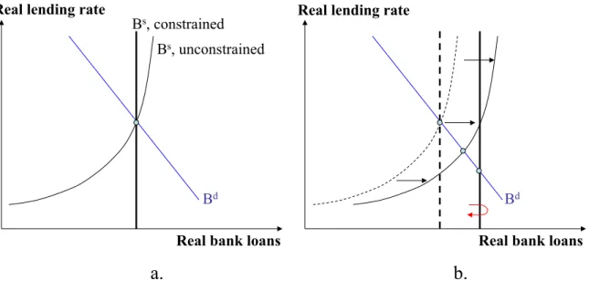
Intuitively, imposing an always binding capital constraint turns an upward-sloping loan supply curve into a vertical one (Figure 1a.). To illustrate the procyclical effect of a fixed capital requirement and the countercyclical property of the Basel III-type requirement in our model, let us assume momentarily that the loan demand schedule
is unaffected by output movements4 and that the output elasticities of loan supply are
the same for the no-capital-requirement case and the fixed-capital-requirement one. The
second assumption5 forces the loan supply schedules in both cases to shift by the same
horizontal distance for a given change in the output amount which together with the first assumption simplifies graphical presentation.
3The latest Basel II announcement leaves open to national authorities as to what should be used
as a conditioning variable for the countercyclical capital buffer. The ideal choice should presumably be the one that best reflects the buildup of system-wide risk. Given that such criterion is irrelevant for the model in this section, we simply follow the literature in using the deviation of GDP from its steady state as the reference cycle.
4This is exactly the condition assumed byCecchetti and Li(2005) for their dynamic model.
5In our model, this is accomplished by setting the elasticity with respect to the output gap of real
deposits equal to that of real bank capital. In reality, the latter is generally larger than the former, implying a larger shift of the vertical supply curve which strengthens the degree of procyclicality induced by the fixed capital requirement.
Real bank loans Real lending rate
Bd
Bs, unconstrained Bs, constrained
Real bank loans Real lending rate
Bd
a.
b.
Figure 1: Loan market equilibrium
From a partial equilibrium perspective, an increase in aggregate economic activ-ity shifts the loan supply schedules in both the unconstrained and the fixed-capital-requirement cases to the right (Figure 1b.). Compared to the unconstrained case, the fixed-capital-requirement case has the loan supply schedule intersect the loan demand schedule at a higher loan amount and a lower real lending rate. Given the specification of aggregate demand, the lower real lending rate would stimulate output even further. Thus, despite the fact that we fix the initial shifts of the two supply schedules to be the same, the final equilibrium in the fixed capital requirement case would have the vertical supply schedule move further rightward due to a multiplier effect.
Having shown the association between one form of financial-sector procyclicality (in which procyclical bank lending amplifies the business cycle) and the fixed capital requirement in our model, we turn to the countercyclical property of a Basel III-typed capital requirement. In this latter case, the required capital ratio rises with an eco-nomic expansion, forcing banks to moderate their loan book expansion and effectively pulling the loan supply schedule back to the left. Compared with those under the fixed-capital-requirement case, the equilibrium bank loans under the countercyclical-capital-requirement case will be lower while the equilibrium loan rate will be higher and as a result output will be less stimulated. Put differently, with countercyclical capital requirement, bank loans will be less procyclical and the business cycle will be less amplified.
Log-linearizing equation2.8 yields
bst =nt−
γ2
γ1c+ 1
xt. (2.9)
yields ωcxt=θxt−1+ (1−θ)Etxt+1−σ(it−Etπt+1) +εt, (2.100) where ωc = 1− ϑ bi nx− γ1γc2+1 −bx
. The superscript c denotes that this is the
capital-constrained case. It is noteworthy here that the presence of a capital constraint affects only the aggregate demand equation, with the aggregate supply equation unchanged.
2.2
Model Parameterization
Rather than estimating the model from the data, we adopt the following calibration strategy. First, we deliberately parameterize relevant parameters in a way that makes
ωu equal to one. With this parameterization, the aggregate demand equation under
the unconstrained case 2.10 becomes isomorphic to a standard hybrid aggregate demand
equation which allows us to adopt certain parameter values that have already been estimated by others. Given that the unconstrained case largely characterizes the real world when viewed over a long time series, our parameterization scheme is not too unreasonable. On the plus side, it allows us to sidestep certain data and estimation issues which are not central to our illustrative analysis while at the same time still providing some realism.
Second, we note that the aggregate demand equation when banks are constrained by a capital requirement differs from the aggregate demand equation when banks are unconstrained (2.1’) in two places: the coefficient on the current output gap and the coefficient on the ex ante real interest rate, of which only the former depends on the degree of countercyclicality of the capital constraint. To highlight their respective implications
on the dynamics of the economy and optimal monetary policy, we also parameterize ωc
whenγ2 = 0 to one so that the aggregate demand equation in the fixed capital requirement
case differs from the unconstrained case only to the extent of interest rate elasticity of output.
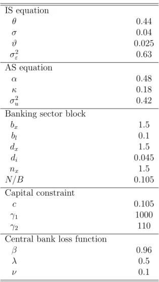
Table 1 lists the values of model parameters. For θ, α, κ, σ2
ε, and σ2u, we use the
values from the estimated euro area model ofEhrmann and Smets(2003). We choose the
Ehrmann and Smets model for our illustrative analysis for two reasons. First, European banks had been at the center of the Basel III discussions before its eventual
announce-ment. Second, the model is in annual frequency which matches the 12-month time
horizon that undercapitalized banks need to meet the additional countercyclical capital
requirement under the Basel III regime. The unconventional parameters ϑ, bx, bi, dx, di
and nx are chosen under the constraints ωu = ωc(γ2 = 0) = 1 and σ + ∆ = 0.06 (the
value of interest elasticity of the output gap in the Ehrmann and Smets (2003) model).
The ratio N/B and c are set to 0.105, the sum of the minimum capital ratio and the
conservation capital buffer under Basel III. This left γ1 and γ2 as the free parameters
Table 1: Baseline parameter values IS equation θ 0.44 σ 0.04 ϑ 0.025 σε2 0.63 AS equation α 0.48 κ 0.18 σu2 0.42
Banking sector block
bx 1.5 bl 0.1 dx 1.5 di 0.045 nx 1.5 N/B 0.105 Capital constraint c 0.105 γ1 1000 γ2 110
Central bank loss function
β 0.96
λ 0.5
ν 0.1
set them equal to 1,000 and 110, respectively, which together with the above parameter
values give γ = 1.3. In obtaining these values, we simulate the model under the
fixed-capital-requirement case 1,000 times and search for γ1 and γ2 that make the simulated
countercyclical capital buffer not only falling within a range of 0-2.5% but also staying
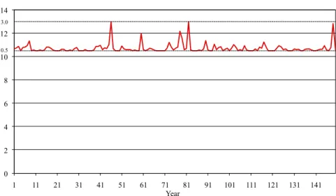
near zero most of the time as prescribed by the Basel III announcement. Figure 2shows
the simulated path of the overall capital requirement for the first 150 time periods.
Finally, we assume for the central banks period loss function that λ = 0.5 and
ν = 0.1 and that the discount factor β = 0.96 given that theEhrmann and Smets(2003)
model is based on annual data.
2.3
A Simple Limiting Case
As a prelude to the simulation results, it is instructive to examine a simple limiting case where a closed-form solution is available. As it is well known, closed-form solutions can be derived when the central bank is not concerned about interest rate variability and the underlying model economy is either purely backward looking or forward looking. Given
0 2 4 6 8 10 12 14 1 11 21 31 41 51 61 71 81 91 101 111 121 131 141
Required capital ratio
Year
10.5 13.0
Figure 2: Simulated capital ratio
that the backward-looking case has been worked out in detail byCecchetti and Li(2005),
we choose the forward-looking case for the analysis in this subsection. In this case, the central bank’s problem is given by
min Lt= 1 2Et ∞ X τ=0 βτ πt2+τ +λx2t+τ (2.10) subject to ωxt=Etxt+1−σ(it−Etπt+1) +εt, (2.11) πt=βEtπt+1+κxt+ut, (2.12)
where, given the aforementioned calibration scheme, ω (unconstrained case) = ω (fixed
requirement case) = 1 < ω (countercyclical requirement case) and σ (unconstrained
case) > σ (fixed requirement case) =σ (countercyclical requirement case). Without loss
of generality, we replace the Phillips curve 2.2 with a standard new Keynesian Phillips
curve 2.12 so as to also enable comparison with a basic new Keynesian model.
It is instructive to iterate equation 2.12 forward to obtain
xt=Et ∞ X τ=0 n − σ ω1+τ(it+τ −πt+1−τ) + εt+τ ω1+τ o (2.13)
Equation 2.13 highlights the monetary transmission mechanism in our model. As in the
basic new Keynesian model, the current output gap depends not only on the current
policy rate but also on its expected future path. What is new according to equation 2.13
policy through a smaller σ and a larger ω which together lower the sensitivity of the output gap to the current and the expected real policy rates.
It is noteworthy that the effect ofσ is constant through time while the effect of ω
increases over time. Mechanically, ω captures the responsiveness of the current output
gap to the expected future output gap, with the larger ω, the smaller the influence of
the latter on the former. This further weakens the link between the expected future policy rates and the current output gap which is central to models with forward-looking features.
On the other hand, a largerω reduces the impacts of the current and the expected
demand shocks on the current output gap. This latter property will become important when we discuss optimal monetary policy for the full model in the next subsection.
For the problem at hand, the solution to the central banks optimization is simple. When the central banks loss function contains only output gap and inflation stabilization objectives and there is no constraint on the zero lower bound (ZLB) on the nominal interest rate, optimal monetary policy calls for a complete offset of the impact of the
demand disturbanceut, leaving the dynamics of the equilibrium output gap and inflation
independent of the aggregate demand equation. More importantly for our analysis, this means that the presence of a capital requirement constraint, whether fixed or countercycli-cal, has no bearing on the equilibrium output gap and inflation processes and consequently the value of the loss function if the central bank conducts its policy optimally. Viewed this way (that the only relevant constraint for the central banks optimization problem
is the aggregate supply curve), the Cecchetti and Li (2005) result that the equilibrium
output gap and inflation processes depend only on the supply shock in a manner that is independent of the capital constraint is not surprising.
It remains to examine the specific form of an optimal monetary policy rule in this simple limiting case. The equilibrium concept we adopt for this purpose is the timeless
perspective commitment equilibrium advocated by Woodford (2003). We note however
that assuming the generally inferior discretion equilibrium does not alter our conclusions about the implications of the capital constraint on optimal monetary policy, whether in this simple limiting case or a more general one.
Under the commitment equilibrium, the equilibrium output gap and inflation pro-cesses are given by
xt=c1xt−1+c2ut, πt= λ κ (1−c1)xt−1− λc2 κ ut, where c1 = 0 < 1+β+κλ2− r 1+β+κλ22−4β 2β <1, c2 =− κ
λ[1+β(1−c1)]+κ2 <0. See Clarida et al.
Using the aggregate demand equation2.11to back out the equilibrium interest rate behavior under timeless perspective commitment yields
it = λ κ (1−c1)− 1 σ(ω−c1) c1xt−1+ λ κ (1−c1)− 1 σ(ω−c1) c2ut+ 1 σεt. (2.14)
Equation2.14reveals two important observations. First, the optimal policy rate response
to a demand shock is larger when the capital constraint is binding (due to a smaller σ).
Intuitively, the presence of a binding capital constraint reduces the ability of the policy rate to neutralize the effect of a given demand shock. So a larger change in the policy
rate is required. The impact of a smaller σ also applies to the policy rate response to a
supply shock although in this case the inflation-output stabilization tradeoff causes the central bank to only partially offset the effect of a supply shock.
Secondly, the more countercyclical the capital requirement is (as captured by a
larger ω), the larger the optimal policy rate response to a supply shock. This is a
consequence of our earlier result that the effectiveness of monetary policy transmission mechanism is further reduced by the degree of countercyclicality of the binding capital constraint.
2.4
Simulation Results
The simple limiting case examined in the previous subsection provides several important insights into how to think about optimal monetary policy conducts in the presence of a binding capital requirement constraint for banks. However, not all of the results of the previous subsection carry to a more realistic setting where the underlying economy exhibits inertia in the output gap and inflation processes and the central bank faces costs of interest rate adjustment. The latter, in particular, renders a complete offset of demand shocks suboptimal. As a result, the equilibrium output gap and inflation processes will necessarily depend on the specification of the aggregate demand equation and hence the form of the capital constraint. It also follows that the value of the loss function will no longer be invariant to the regulatory regime.
Under commitment, the optimal policy rules and their associated losses in the calibrated model are given by
Unconstrained (loss=42.28)
it= 0.58it−1+ 0.60xt−1+ 0.38πt−1+ 1.37εt+ 0.78ut−0.62Ξx,t−1−0.22Ξπ,t−1 Fixed capital requirement (loss=48.38)
Fixed capital requirement (loss=45.84)
it= 0.71it−1+ 0.35xt−1+ 0.68πt−1+ 0.80εt+ 1.41ut−0.38Ξx,t−1−0.23Ξπ,t−1
where Ξx and Ξπ are the Lagrange multipliers on the aggregate demand equation and
the aggregate supply equation, respectively.
In all three cases, the optimal policy rules call for an increase in the policy rate in response to both positive output gap and inflation developments as captured by their coefficients on the lagged output gap, lagged inflation, and the two stochastic disturbances. With respect to a cost shock, the result is the same as in the simple limiting case. Specifically, the optimal interest rate response to a cost shock when the capital requirement is countercyclical is more aggressive than when the capital requirement is constant, which in turn is more aggressive than when banks are unconstrained. The difference from the simple limiting case is with respect to an optimal interest rate response to a demand shock. It is no longer the case that the optimal policy response to a demand shock is invariant to the degree of countercyclicality of the binding capital constraint. Indeed, for the baseline parameterization, an optimal rate response to a demand shock in the presence of a binding countercyclical capital requirement is even smaller than the unconstrained case.
When the dynamics of the economy depends also on the aggregate demand equation, the benefit of a countercyclical capital requirement comes into play. An important insight from the simple limiting case is that countercyclical capital requirement reduces the impact of a demand shock on the current output gap. This property is inconsequential when demand shocks are completely offset. In the present case where there are residual demand shocks, requiring banks to hold more capital during an economic expansion thus aids the central banks aggregate demand management.
In terms of central banks losses, the loss is the smallest when there is no capital constraint, followed by the countercyclical-capital-requirement case, with the fixed-capital requirement case delivering the largest loss. This ordering should not be interpreted as the unconstrained case being the first best and the countercyclical-capital-requirement case as the second best however. Later when we analyze the optimal degree of countercyclicality of the capital constraint, we will show that there are instances in which a countercyclical capital requirement is associated with a smaller loss than having no constraint at all. Rather, the key message here is that, despite the fact that a countercyclical capital requirement weakens the transmission mechanism of monetary policy relative to a fixed capital requirement, in the end the central bank is better off with a countercyclical capital requirement than with a fixed capital requirement.
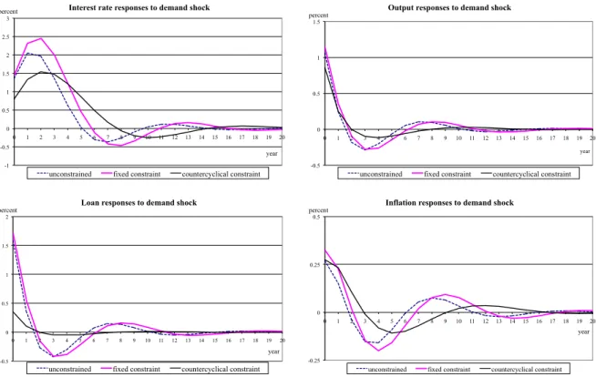
Figure 3 shows the impulse responses of the policy rate, the output gap, bank loans, and inflation to a unitary positive demand shock for the unconstrained case, the
fixed--1 -0.5 0 0.5 1 1.5 2 2.5 3 0 1 2 3 4 5 6 7 8 9 10 11 12 13 14 15 16 17 18 19 20 percent year
Interest rate responses to demand shock
unconstrained fixed constraint countercyclical constraint
-0.5 0 0.5 1 1.5 2 0 1 2 3 4 5 6 7 8 9 10 11 12 13 14 15 16 17 18 19 20 percent year
Loan responses to demand shock
unconstrained fixed constraint countercyclical constraint
-0.5 0 0.5 1 1.5 0 1 2 3 4 5 6 7 8 9 10 11 12 13 14 15 16 17 18 19 20 percent year
Output responses to demand shock
unconstrained fixed constraint countercyclical constraint
-0.25 0 0.25 0.5 0 1 2 3 4 5 6 7 8 9 10 11 12 13 14 15 16 17 18 19 20 percent year
Inflation responses to demand shock
unconstrained fixed constraint countercyclical constraint
Figure 3: Impulse responses to a unitary demand shock
capital-requirement case, and the countercyclical-capital-requirement case. As would
have been expected from the preceding discussion, the initial policy response is mildest in the countercyclical-capital-requirement case. That output and bank loans also fluctuate less in this case is also evidenced by their impulse responses. Through the presence of the lagged output gap term in the hybrid aggregate demand equation, a countercyclical capital constraint also reduces the persistence in output gap movements. This further lessens the impact of demand shocks on the output gap and accordingly bank loans. Finally, while inflation in the countercyclical-capital-requirement regime is less volatile than that in the fixed-capital-requirement regime, it is more volatile than that in the unconstrained regimes which causes the associated policy response to persist longer. This is the adverse consequence of countercyclical capital requirement. Put simply, there is no free lunch. While countercyclical capital requirement helps moderate the impact of demand shocks on output, it reduces the ability of the central bank to control inflation through the weakened monetary transmission mechanism.
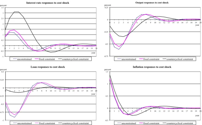
The contrast between the benefit and the cost of a countercyclical requirement on macroeconomic dynamics is most visible in Figure 4 which traces out the impulse responses of the policy rate, the output gap, bank loans, and inflation to a unitary cost shock. In the countercyclical-capital-requirement case, a cost shock invokes a very strong policy response, twice to three times as much as the other cases under the given parameterization. Even with such a strong response, inflation remains the most volatile in the countercyclical-capital-requirement case. On the other hand, both the output gap
-1 -0.5 0 0.5 1 1.5 2 2.5 3 3.5 0 1 2 3 4 5 6 7 8 9 10 11 12 13 14 15 16 17 18 19 20 percent year Interest rate responses to cost shock
unconstrained fixed constraint countercyclical constraint
-1 -0.75 -0.5 -0.25 0 0.25 0.5 0 1 2 3 4 5 6 7 8 9 10 11 12 13 14 15 16 17 18 19 20 percent year Loan responses to cost shock
unconstrained fixed constraint countercyclical constraint
-0.75 -0.5 -0.25 0 0.25 0 1 2 3 4 5 6 7 8 9 10 11 12 13 14 15 16 17 18 19 20 percent year
Output responses to cost shock
unconstrained fixed constraint countercyclical constraint
-0.5 0 0.5 1 1.5 0 1 2 3 4 5 6 7 8 9 10 11 12 13 14 15 16 17 18 19 20 percent year Inflation responses to cost shock
unconstrained fixed constraint countercyclical constraint
Figure 4: Impulse responses to a unitary cost shock
and bank loans are less variable with a countercyclical capital constraint.
Putting all these pieces together, the output gap is least volatile with a counter-cyclical requirement, followed in order by the unconstrained case and the fixed-capital-requirement case. On the other hand, inflation is most volatile with a countercyclical requirement followed in order by the fixed-capital-requirement case and the unconstrained case. That is, countercyclical capital requirement is good for output gap stabilization but bad for inflation stabilization.
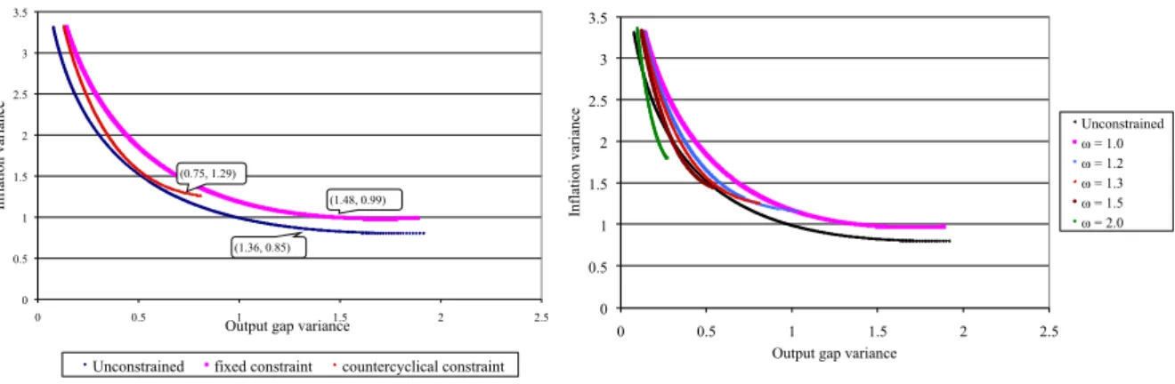
In light of the differential impacts of a countercyclical capital requirement constraint on output and inflation variability, it is natural to examine the output-inflation variability
tradeoff advocated by Taylor(1979) for comparison of alternative monetary policy rules.
Figure 5a plots combinations of the unconditional variances of the output gap and
inflation obtained by varying the central banks weight on output gap stabilization (λ)
from 0 to 100 under the three cases of interest. Also labeled in the figure are the points
on each of the tradeoff frontier for the baseline parameterization (λ = 0.5). Figure 5b
superimposes on Figure 5a additional tradeoff curves associated with different values of
ω.
Figure 5 highlights several important results. First, under the baseline param-eterization, the output-inflation variability tradeoff under the countercyclical-capital-requirement case dominates the fixed-capital countercyclical-capital-requirement case, but is dominated by the unconstrained case. That is, under the baseline parametrization, the unconstrained case dominates the two capital-constrained cases in terms of both the central banks loss and the
0 0.5 1 1.5 2 2.5 3 3.5 0 0.5 1 1.5 2 2.5 Infl at ion va ri anc e
Output gap variance
Unconstrained fixed constraint countercyclical constraint
(0.75, 1.29)
(1.36, 0.85)
(1.48, 0.99)
a. Baseline parameterization b. Effects of increased countercyclicality
0 0.5 1 1.5 2 2.5 3 3.5 0 0.5 1 1.5 2 2.5 Infl at ion va ri anc e
Output gap variance
Unconstrained ! = 1.0 ! = 1.2 ! = 1.3 ! = 1.5 ! = 2.0
Figure 5: Output-inflation variability tradeoff
output-inflation variability tradeoff. The same however cannot be said for high degrees of requirement countercylicality. As the degree of countercylicality of a capital requirement
increases, the tradeoff frontier pivots to the left. For high values of ω, parts of the
tradeoff frontiers even lie below the tradeoff frontier under the unconstrained case. The
superior tradeoff at high values ofω however comes at the expense of higher interest rate
volatility (simulation results not shown). So it is not clear whether a higher degree of countercyclicality will always be preferred by an optimizing central bank. Subsection 2.6 will take on this issue in detail. Finally, a countercyclical capital constraint shortens the
variability frontier. The higher the value of ω, the shorter the tradeoff curve and the
higher the minimum level of inflation variability a central bank can achieve. This is the consequence of our earlier finding that countercyclical capital requirement interferes with
the central banks inflation stabilization. For an inflation nutter (King (1997)), a fixed
capital requirement may be preferred to a countercyclical one.
2.5
Countercyclical Capital Requirement and Optimal Taylor
Rules
A large part of the modern monetary policy literature chooses to focus on simple
instru-ment rules like the so-called Taylor (1993) rule that responds to only contemporaneous
the output gap and inflation as opposed to complicated optimal commitment rules. The justifications are that in many cases simple Taylor-like rules yield similar macroeconomic stability to optimal commitment rules and are also a reasonable approximation of actual policy making. It is therefore of interest to also examine the implications of countercycli-cal capital requirement on the form of optimal Taylor rules and their performances using the same loss function as in the previous subsection.
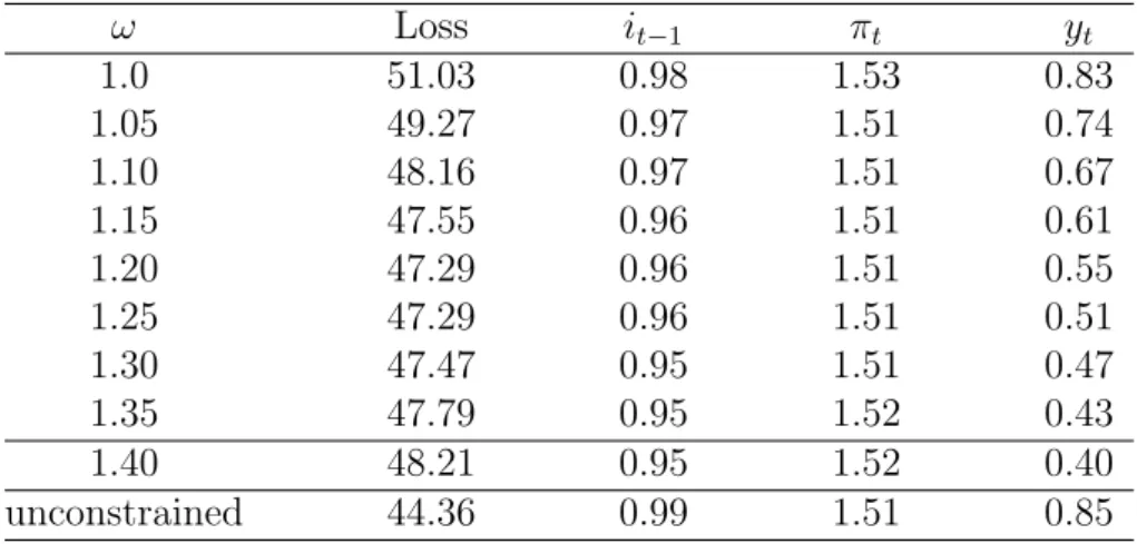
Table2reports the value of the loss function and the optimal reaction coefficients of
for the unconstrained case is also reported in the last line of the table for comparison.
Table 2: Optimal Taylor rules and degree of countercyclicality
ω Loss it−1 πt yt 1.0 51.03 0.98 1.53 0.83 1.05 49.27 0.97 1.51 0.74 1.10 48.16 0.97 1.51 0.67 1.15 47.55 0.96 1.51 0.61 1.20 47.29 0.96 1.51 0.55 1.25 47.29 0.96 1.51 0.51 1.30 47.47 0.95 1.51 0.47 1.35 47.79 0.95 1.52 0.43 1.40 48.21 0.95 1.52 0.40 unconstrained 44.36 0.99 1.51 0.85
Several observations deserve to be highlighted. First, asω increases from unity, the
central banks loss becomes smaller. However, after a certain point, the value of the loss picks up again, suggesting that there is an optimal degree of countercyclicality of the capital constraint. This issue will be explored further in the next subsection.
Second, the optimal coefficients on the lagged interest rate and inflation do not changed much with the degree of countercyclicality. This observation is in sharp contrast with the third observation which concerns the optimal coefficient on the output gap. For
the baseline parameterization (ω = 1.30), the optimal coefficient on the output gap falls
by nearly a half from 0.83 to 0.47 from the fixed-capital-requirement case (ω = 1). The
reduced output response is a reflection of our earlier result that the greater the degree of countercyclicality of a capital requirement, the smaller the need for the central bank to stabilize output.
Given the significant impact of the degree of countercylicality on the optimal Taylor rule, it is of interest to see what will happen to the equilibrium outcomes if the central bank is not aware of the implications of the countercyclical capital constraint on the dynamics of the economy and remains committed to the optimal Taylor rule for the unconstrained case. In this case, the central banks loss and the unconditional variances of the output gap, inflation, and the policy rate are respectively 47.87 (compared to 47.47), 0.68 (compared to 0.72), 1.37 (compared to 1.36), and 21.32 (compared to 20.26). Qualitatively, by committing to the Taylor rule under the unconstrained case, the central bank overreacts to output gap developments. The central banks non-optimizing behavior brings down output gap variability at the expense of both inflation variability and interest
rate variability. Overall, the latter two outweighs the former, resulting in a larger
loss for the central bank. Nevertheless, the loss differential is only about one percent, suggesting that the central banks failure to internalize the implications of the binding capital constraint may not matter much quantitatively.
2.6
Optimal Degree of Countercyclicality
The analysis thus far concerns optimal monetary policy for a given degree of capital requirement countercyclicality. This subsection takes one step further to examine the
optimal policy combination. This problem is best addressed by assuming, not too
unrealistically, that the central bank is also in charge of the capital buffer calibration. In the context of our model, the central bank would at the outset fix the desired degree of countercyclicality of the capital buffer in conjunction with monetary policy to minimize
the value of the loss function.6
For ease of exposition, we assume that the central bank chooses directly the
pa-rameterω as the additional choice variable. The optimal value ofω will likely depend on
several parameters. Rather than providing a full set of comparative statics, this subsection mentions two considerations that are likely to be of high practical importance.
The first consideration is the relative magnitude of the variances of the demand and the cost shocks. An important result from the earlier subsections is that countercyclical capital requirement is good for offsetting the impact of demand shocks but bad for the performance of monetary policy in the face of supply shocks. Therefore, the optimal degree of countercyclicality in an economy where supply disturbances dominate will be lower than that in an economy where demand disturbances dominate, holding other things equal.
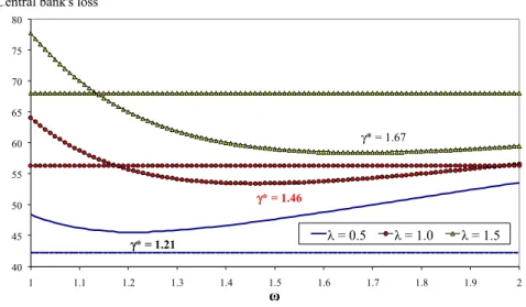
The second consideration concerns the weight the central bank places on output gap stabilization. Because countercyclical capital requirement helps the central bank stabilize the output gap at the expense of inflation stabilization. The optimal degree of countercyclicality should be higher as the central banks weight on output gap stabilization
increases. Figure 6 confirms this intuition. The optimal value of ω indeed rises with the
value of λ. For our baseline parameterization where λ = 0.5, the optimal value of ω is
1.21, below our baseline value of 1.30.7 For λ = 1.0 (the central bank places an equal
weight on output and inflation stabilization), the optimal value of ω is 1.46.8
Figure 6 also illustrates another important point. When λ is high enough, it is
possible for the central bank to achieve a lower level of loss with a countercyclical capital requirement than without a capital constraint at all. Thus, provided that the central banks objective function approximates well the true social preference, in certain societies,
6An alternative approach is to assume a separate macroprudential authority engaging in
cooperative/non-cooperative games with a central bank. SeeAngelini et al.(2010) for an application of this approach.
7The loss differential however is marginal (45.56 versus 45.84), suggesting that over a certain range,
the degree of countercylicality does not matter much to the central banks loss.
8Interestingly, the optimal value of ω for an inflation nutter central bank (λ = 0) is 0.74,
implying that the optimal capital requirement is procyclical. The threshold λ that makes a fixed requirement optimal is 0.17. These conclusions however ignore the financial stability benefit of capital requirement countercyclicality and the financial stability cost of increase bank lending procyclicality which conceptually should result in a higher value of optimalω.
40 45 50 55 60 65 70 75 80 1 1.1 1.2 1.3 1.4 1.5 1.6 1.7 1.8 1.9 2
Central bank's loss
!
! = 0.5 ! = 1.0 ! = 1.5
!* = 1.21
!* = 1.46
!* = 1.67
Figure 6: Central bank’s loss
particularly ones that may care strongly about output stabilization, implementing an appropriately calibrated countercyclical capital buffer is ultimately welfare improving.
3
Policy Coordination in a Model with Financial
In-stability
As insightful as it is, the model of the preceding section lacks one important dimension: financial stability – the very objective of macroprudential regulation. There is neither boom/bust nor bank failure associated with the bank lending cycle generated by the assumed simple banking sector block. The use of a macroprudential tool (the counter-cyclical capital buffer) to restrain bank lending behavior in that model is solely for the sake of economic stabilization and not for the resilience of the financial system as strongly emphasized by the post-crisis consensus.
Unfortunately, when it comes to financial stability modeling, there is no standard canonical model to rely on for policy analysis. In particular, models based on a dynamic general equilibrium concept, whether the likes of the model in the preceding subsection
or their larger DSGE cousins, are generally poor at incorporating financial instability.9
This section thus opts for an alternative model that is less conventional but richer in financial stability dimension.
Our model relies on two central elements in explaining the emergence of financial instability. The first is the basic procyclicality mechanism which works to propagate and magnify shocks, while the second, the path dependence feature, enables the degree of
9Two notable exceptions areFilardo(2007) for a small model andGertler and Kiyotaki(2010) for a
procyclicality to accumulate over time. Specifically, when the strength of procyclicality itself is procyclical (namely it rises with positive shocks), a boom automatically increases the degree of financial fragility, sowing the seed for an outsized crash later on once the shock dissipates. Given these two mechanisms, mere temporary shocks can lead to bubble-and-crash phenomena.
Technically, the source of basic procyclicality in our model derives from the
mark-to-market and banks’ balance sheet adjustment mechanism, described byShleifer and Vishny
(2010) andAdrian and Shin(2010). We extend their work by highlighting that, when the
model is cast in a dynamic setting, there is a path dependence feature: as balance sheet size expands, the sensitivity to mark-to-market gains or losses grows, which captures the idea of time-varying financial fragility. A positive shock to asset price raises banks’ capital via a mark-to-market gain, which encourages further balance sheet expansion and brings about increased fragility. When the shock dissipates, the high level of asset price becomes unsustainable and the correction necessarily excessive due to the accumulated fragility during the run-up.
It will be shown that, in this context, the use of policy interest rate (or indeed any discretionary monetary policy) in pursuit of financial stability is subject to a number of severe limitations. On the other hand, macroprudential regulation in rule-based form, which has a structural and long-term objective in mind, can help weaken the degree of procyclicality and arrest the risk of financial instability at source. While macroprudential tools may vary, they should share a common objective of ensuring a structurally more resilient financial system.
3.1
The Model
There is a single asset in the economy, in fixed supply of size N. The asset is the
securitized loans extended to the real sector, and the banks’ loan supply is modeled
as the demand for this asset10. Banks finance their asset holdings from either equity
or short-term debt. The asset can also be bought by passive investors, whose asset
demand function slopes downward with asset price. Time is discrete and divided into
three periods, t ∈ {1,2,3}. At time t, denote asset’s price by pt, banks’ total holding of
asset by nt, banks’ equity byet, and banks’ liability bydt. The asset market equilibrium
condition requires that the sum of demand for assets from banks and passive investors
equals the total supply N in each period. In period 1, the equilibrium asset price and
banks’ asset holdings are exogenously given (which is consistent with a steady state, to be defined later).
10See Bernanke and Blinder (1988) for a similar approach. This assumption is made purely for
convenience, to bypass explicit modeling of borrowers. For a predominantly non-securitized banking system, the assumption should be interpreted as saying banks have an exposure to the asset that their borrowers invest in for instance through the collateral value.
In the beginning of periods 2, the central bank designs policy configuration before observing shocks. The permissible class of policy instruments includes (1) the policy
interest rate it and (2) regulatory requirements that set limits on banks’ total asset or
leverage. In period 2, the asset market is then subject to a temporary shock, modeled as a shift in passive demand, causing the asset market to re-equilibrate. In the final period, the passive demand returns to its original position, and the asset market is allowed to go
through final adjustment. We will distinguish between a nimble policy maker who can
reset its policy in period 3, and a clumsy who cannot do so as it is constrained by the
long lag with which the policy instrument works.
At the end of the final period, the asset yields a return randomly drawn from a distribution with known expected value. Passive investors are risk-averse and therefore scale down their asset demand as price rises, in line with lower risk-adjusted expected return. A higher interest rate raises return on a competing risk-free asset, and lowers
passive demand for assets. Passive demand, denoted by t(it, pt) ∈ [0, N], is therefore a
decreasing function of both price and policy interest rate.
Banks only invest in one type of asset, therefore their asset demand is effectively their balance sheet size. Banks are risk-neutral and aim to maximize the net present value of investment. The asset’s expected return is assumed to be sufficiently large such that the net present value is always positive, so that banks would always want to raise more debt to increase their asset holding. Their ability to issue debt is however constrained by their
capital endowment. Specifically, in period t banks need to maintain a capital-to-asset
ratio of ht(it), an increasing function of interest rateit, namely
et
et+dt
=ht(it) (3.1)
Clearly, the inverse 1/ht(it) is simplyleverage ratio.
We choose to remain agnostic about the exact source and functional form ofht(it),
except that∂ht(it)/∂it >0 for anyt,11and instead focus on the role that leverage plays in
transmitting the effect of monetary policy to asset market equilibrium. We letht depend
11The micro-foundation forh
t(it) can be motivated in a number of ways. In the presence of asymmetric information and agency costs, ht(it) can be interpreted as the creditors’ demand that banks hold a sufficient level of capital in order to retain enough ‘skin in the game’ for effort to be credible in the spirit
of Holmstrom and Tirole (1997). Higher interest rate lowers returns to asset in present value terms,
making agency cost more binding and hence forcing banks to hold more capital. In this sense, the ratio ht(it) is ahaircut required by banks’ creditors. Shleifer and Vishny(2010) adopt this interpretation and consider the special case of constant ht(it) = h. An alternative interpretation is that ht(it) is chosen voluntarily by banks to meet some objective; for instance inAdrian and Shin(2010), banks aim to stay afloat in each period by holding enough capital to cushion against the worst-case loss. In their model, ht(it) is then derived from the value-at-risk constraint that banks strive to meet in each period. Higher interest rate lowers the present value of asset return, raising the worst case loss and making the value-at-risk constraint more binding. More generally, the dependence of ht(it) onit can also be interpreted as a representation of the ‘risk-taking’ channel of monetary policy transmission (Borio and Zhu(2008)). In any interpretation,∂ht(it)/∂it>0, for anyt.
on time t solely to allow for the possibility of discretionary regulatory policy effecting
change on banks’ leverage so that, for fixed it = i, h1(i) =6 h2(i) 6= h3(i). Absent this
regulatory policy action, we assume thath1(i) =h2(i) = h3(i) for any giveniso that there
is no inherent ‘leverage cycle’ in our model (unlike the mechanism inGeanakoplos(2009),
for example, where leverage is time-varying indicating shifts in risk-taking behavior).
The asset price pt and the amount of net asset buying/selling by banks are
deter-mined by the market equilibrium condition, which in turn defines the state variables’
dynamics. The net asset buying in equilibrium, denoted by Bt, is financed by more
borrowing, hence:
dt=dt−1+ptBt (3.2)
At the beginning of each period, banks’ assets are marked to market and any price appreciation increases the equity value of the banks:
et=nt−1pt−dt−1 (3.3)
3.2
Genesis of Financial Instability
Let us begin by formulating the asset market equilibrium condition. Substituting
equa-tions 3.2 and 3.3 into3.1, we get
ht(it) =
nt−1pt−dt−1
pt(nt−1+Bt)
(3.4)
Invert this, using the balance sheet identity dt−1 ≡(1−ht−1(it−1))nt−1pt−1 and the asset
size identity nt≡nt−1+Bt, we obtain banks’ asset demand function
nt(it, pt) = nt−1 ht(it) 1− pt−1 pt (1−ht−1(it−1)) (3.5) for 0≤nt≤N.
Banks’ and passive investors’ demand together make up the total asset demand. The asset market clears when the total asset demand equals asset supply, i.e.
N =t(it, pt) +nt(it, pt) (3.6)
We now consider the implications of the model within period (static) and across periods (dynamic), respectively. To focus attention on the inherent properties of the asset market
equilibrium, we will assume fixed policy, i.e. ht(it) = h for all t, throughout the rest of
N
Banks' asset holding Passive asset holding
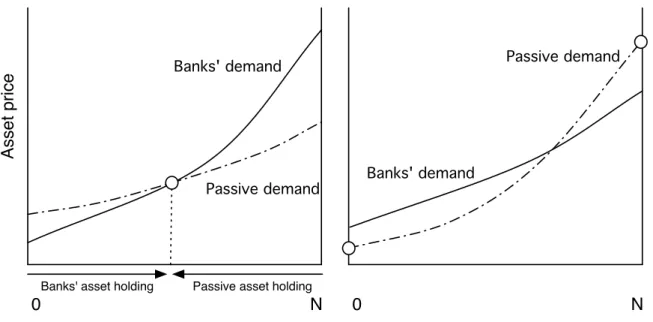
Asse t p ri ce 0 Banks' demand Passive demand N 0 Banks' demand Passive demand
Figure 7: Procyclicality and Static Implications
3.2.1 Propagation and indeterminacy
It is evident from equation 3.5 that banks’ demand function is upward sloping in asset
price. This unorthodox shape of the demand curve stems from marking to market
originating in equation 3.3, whereby a rise in asset price induces a capital gain accrued
to banks, strengthening their balance sheets and allowing them to increase asset holdings while still respecting the leverage constraint. The upward-sloping demand is the basic procyclicality engine in our model. Any shock that induces price appreciation is amplified by the expansion of banks’ balance sheets and debt accumulation. When procyclicality is strong enough, self-fulfilling expectations may take over fundamentals, as we now show.
The determination of asset market equilibrium is schematically illustrated in Figure
7. In both panels, the asset demand by banks should be read from left to right, while
passive demand from right to left. The intersection point of the two demand curves defines the market equilibrium. Consider first the left panel, in which there is a unique interior stable equilibrium. Because of banks’ upward-sloping demand function, a shock that induces an upward shift in the passive demand curve, say by ∆, would lead to a larger-than-∆ increase in the equilibrium asset price. In contrast, if both demand functions were downward sloping, the increase in asset price would have been less than one-for-one. Moreover, the passive investors end up holding less assets in the new equilibrium despite the initial demand shift. This is because they are priced out of the market by banks, who, in response to the initial price rise, manage to raise asset demand via stronger balance sheets.
A unique stable equilibrium is not the only possibility. In the right panel of Figure
positive excess demand, putting further upward pressure on price. In this case, there are two stable equilibria, both of which are corner solutions where banks either price all passive investors out totally, or exit the market altogether. Which equilibrium will be borne out is indeterminate. The indeterminacy can be interpreted as an extreme form of uncertainty, as the procyclicality from marking to market becomes so strong that the asset price and banks’ investment can swing from self-fulfilling expectations without any change in fundamentals.
A unique stable equilibrium can be guaranteed provided this procyclicality is not too strong, i.e. if banks’ asset demand does not rise too quickly with price. This will
ensure that the excess demand function, t(i, pt) +nt(i, pt)−N, is monotone decreasing
in price and hence cuts zero from above at most once. A precise sufficient condition for a unique stable equilibrium is that banks’ demand function be a “contraction” of passive
demand. That is, there exists k <1 such that, for any p1, p0 ≥0,
nt(i, p1)−nt(i, p0) ≤k t(i, p1)−t(i, p0) (3.7)
Under this condition, uniqueness of a stable equilibrium can be established using
argu-ments akin to contraction mapping theorem.12 Intuitively, this condition requires that, as
asset price rises, banks’ demand for asset climbs more slowly than passive demand falls. In other words, banks’ demand function is flatter (and inverse demand function steeper)
than that of passive investors, as depicted on the left panel of Figure 7.
Leverage is an integral determinant of the strength of procyclicality, as the next result establishes.
Proposition 1. The slope along any two points of banks’ demand is decreasing in h.
Proof. The objective is to establish that, for any arbitraryp1 andp0,|n
t(i, p1)−nt(i, p0)|
is decreasing in h. Using equation 3.5, we have
nt(i, p1)−nt(i, p0) = nt−1pt−1 p0 1−h h − nt−1pt−1 p1 1−h h =nt−1pt−1 1 h −1 1 p0 − 1 p1
12Assume a continuous excess demand functiont(i, p
t) +nt(i, pt)−N : [0,∞]7→[−2N,2N] that cuts zero at least once so that an equilibrium always exists. For no loss of generality, consider any arbitrary pair of pricesp0< p1. Since banks’ demand slopes upwards while the passive demand slopes downwards,
condition3.7implies that
nt(i, p1)−nt(i, p0)< t(i, p0)−t(i, p1) t(i, p1) +nt(i, p1)−N < t(i, p0) +nt(i, p0)−N
That is, any part of the excess demand function is always downward-sloping in price. The method of successive approximations can be employed to solve for a unique stable equilibrium, akin to how a unique fixed point is guaranteed in the contraction mapping theorem.
which is decreasing in h for any p1 and p0.
An immediate implication is that, the uniqueness condition 3.7 is more likely to
fail with higher leverage. Intuitively, higher leverage raises the strength of balance sheet valuation mechanism, enabling banks to expand debt-financed asset purchase following any price increase. Underlying this mechanism is an externality, as one bank’s increased asset demand pushes price up, allowing other banks to purchase more asset and so on. This results in higher sensitivity of market equilibrium to fundamental shocks such as changes in passive demand. It is in this sense that higher leverage is associated with more procyclicality. As leverage grows sufficiently high, the spillover effect between banks becomes so strong that coordination problem emerges: each bank will purchase more
asset if it believes other banks will also do so, but will sell otherwise.13
Procyclicality in this form presents a challenge to the policy maker. If adjustments in monetary policy, either via policy interest rate or through macroprudential regulation,
are not large enough to raise h above the range that can support multiple equilibria,
monetary policy can be ineffective. The market equilibrium in this case will solely be
a function of self-fulfilling expectations rather than h that the policy maker may be
adjusting to no avail.14 For monetary policy to have an effect, the policy adjustment
must be large enough to ensure that the contraction condition 3.7 holds. With strong
procyclicality, the transmission of monetary policy can be highly nonlinear.
The potential ineffectiveness of policy interest rate alone provides a powerful ra-tionale for adopting an alternative and more coercive measure such as regulatory policy. Indeed this is one of the oft-cited reasons when some central banks adopt macroprudential measures to control financial excesses. But, perhaps less obviously, even with a unique equilibrium, the balance sheet mechanism remains a potent source of complex procycli-cality that can pose threat to financial stability in a non-trivial way. To pursue this issue at greater length, henceforth it will be assumed that the condition for equilibrium uniqueness is always satisfied throughout and multiplicity never arises.
3.2.2 Path dependence and dynamic implications
Equation3.5shows that banks’ demand function exhibitspath dependence property, since
the current demandnt depends onpt−1 andnt−1 in addition to the current pricept. Past
equilibrium therefore has bearing on the current demand. As an illustration, consider
the following two limiting cases. As pt→ ∞, the asset demand asymptotes tont−1/h, so
13The association between strong strategic complementarities and multiple equilibria is
well-documented in the literature, see for exampleCooper and John (1988).
14In a more elaborate model, e.g. one equipped with an equilibrium selection mechanism, it may
be argued that monetary policy works by changing the relative sizes of the basins of attractions, which makes one equilibrium more likely than the other. The market equilibrium in that model, while unique, will still be insensitive to monetary policy for small policy adjustments.
a larger asset holding in the last period would boost the current demand. On the other
hand, the intercept of the inverse demand function (the priceptat which nt= 0) is given
by pt−1(1−h), so that a higher equilibrium price in the last period would raise inverse
demand function (i.e. a drop in demand). These limiting cases suggest that the past equilibrium affects the current asset demand by ‘rotating’ the demand schedule. We will now characterize these rotational adjustments in demand curve more precisely using the idea of contraction, and show how they give rise to non-trivial dynamic implications.
The key result of this section can be understood intuitively. Asset price and asset holding jointly determine banks’ initial balance sheet size, which in turn dictates the strength of balance sheet mechanism and resulting degree of procyclicality. Stronger procyclicality is associated with a flatter of banks’ demand schedule, indicating higher demand elasticity with banks increasing their demand by more in response to a price rise. While higher elasticity implies stronger propagation of any positive shock to asset price, it also implies more vulnerability to any negative price shock. With this mechanism at work, financial instability can simply be induced by a positive transitory shock to price. A positive shock leads to the expansion of banks’ balance sheet, which raises procyclicality and leaves the asset market highly vulnerable. A reversal in shock, due to its transitory nature, is therefore sufficient to result in an outsized downward adjustment in asset price as banks scramble to sell asset in a falling market. The evolution of asset market adjustments therefore closely mimics the build-up of bubbles and the subsequent crash. This is our basic story of how financial instability emerges.
We begin our formal discussion of the model’s dynamics and implications by first establishing the existence of steady states and characterize their properties.
Steady states
A steady state is defined as a sequence of equilibrium outcomes in which the pair
{nt, pt} is fixed over time, and equal to some constant {n∗, p∗}. In other words, in
a steady state equilibrium, both passive and banks’ demand schedules must be time
invariant. But it is evident from equation3.5 that, for a given history of past equilibrium
{nt−1, pt−1}, there is a unique pair on the banks’ demand schedule that can be upheld
as a steady state equilibrium, namely {nt, pt} = {nt−1, pt−1} = {n∗, p∗}. This steady
state can then be attained under some passive demand schedule t(i, p) that leads to the
equilibrium pair{n∗, p∗}. This establishes the existence of a steady state. An alternative
way to characterize a steady state equilibrium, is to take passive demand function as
given. Any pair{nt, pt}on the passive demand schedule is consistent with a steady state
corresponding to the history {nt−1, pt−1}={nt, pt}={n∗, p∗}.
There are clearly an infinite number of possible steady states. A formal welfare evaluation between different steady states is beyond our scope, and instead focus will be on short-run equilibrium dynamics after a steady state is perturbed by shocks. We assume that the initial steady state is already welfare-maximizing, and that the policy
N Asse t p ri ce 0 D D E E A B C
Figure 8: The lasting impact of temporary shock
maker’s problem is to stabilize the economy around this initial steady state.15
Shocks and instability
Figure 8 depicts the asset market equilibrium. All variables are predetermined in
period 1, and we are interested in the evolution of asset market equilibrium in periods 2
and 3. The initial equilibrium at point A, {n∗1, p∗1}, coincides with a steady state which,
in the absence of any further shock, would imply n∗1 =n2 = n3 and p∗1 =p2 = p3. The
corresponding banks’ demand schedule is represented by the curve D-D. Assume that in period 2 the passive demand schedule is subject to a positive temporary shock that causes it to shift upwards, before falling back to its original position in period 3. That is
Passive demand in period t=t(i, pt) +ct (3.8)
where c1 = c3 = 0 and c2 > 0. How would this period-2 temporary shock affect the
dynamics of asset market equilibrium?
Given that the initial equilibrium at point A is a steady state, banks’ demand function remains unchanged in periods 1 and 2, before endogenously adjusting in period 3. In period 2, the upward shift in passive demand bids up the asset price, which in turn leads to banks’ capital gain and higher demand for asset that pushes asset price
up further. The equilibrium in period 2 is at point B, in which both asset price p∗2 and
banks’ asset holding n∗2 are now higher than at the initial steady state A.
15In a fuller model, the welfare-maximizing steady state may be one in which the market correctly
prices risks associated with the asset’s return. In this case, the risk-return profile of the asset as well as the social welfare function must be spelled out. Alternatively, the society may wish to maximize the asset price in equilibrium (thereby minimizing the real sector’s borrowing cost) while maintaining the banks’ zero profit condition.