Gender Differences in Full-Time
Self-Employment
Suzanne Heller Clain
This analysis reveals interesting gender differences in full-time self-employment. Women who choose full-time self-employment have personal characteristics that are less highly valued in the marketplace than women who work full-time in wage-and-salary employ-ment. The reverse is true for men. It is unclear whether the gender gap in self-employment income is the result of different supply decisions made by women, or greater constraints and/or discriminatory elements faced by women. There is some suggestion that women may place a higher value on nonwage aspects of self-employment than men do. © 2000 Elsevier Science Inc.
Keywords: Self-employment; Gender differences JEL classification: J23, J16, J30
I. Introduction
In this paper, gender differences in the propensity for self-employment (vs. wage-and-salary employment) and in the levels of earnings in each type of employment are investigated, using econometric techniques. It is found that women who choose self-employment have personal characteristics that are less highly valued by the market than women who choose wage-and-salary employment; the reverse is true for men. Certain personal characteristics appear to affect self-employment earnings differently for women than for men. It is unclear whether the resulting gender gap in self-employment earnings is the result of different supply decisions made by women or the result of greater constraints and/or discriminatory elements faced by women. Finally, the observed gender differences in the gap between self-employment earnings and potential wage-and-salary income suggest that employed women may place a higher value on the nonwage aspects of self-employment than self-employed men do.
Associate Professor, Villanova University, Villanova, PA.
Address correspondence to: Suzanne Heller Clain, Associate Professor, Department of Economics, Villanova University, 800 Lancaster Avenue, Villanova, PA, 19085.
Journal of Economics and Business 2000; 52:499 –513 0148-6195 / 00 / $–see front matter
A review of the relevant literature is presented in Section II. A discussion of the methodology used in this paper is contained in Section III. Section IV provides a description of the data used, whereas the empirical findings are outlined in Section V. The main conclusions and implications of this research appear in Section VI.
II. Literature Review
The issue of self-employment has attracted the attention of economic researchers in the past decade for various reasons. Some economists have been drawn to the topic by the expansion of the self-employed sector that began in the U.S. in the mid-1970s (Blau, 1987; Evans and Leighton, 1989; Devine, 1994a, 1994b). Others have been interested in the self-employment of marginalized groups (Moore, 1983a; Bates, 1997; Borjas and Bronars, 1989; Fairlie and Meyer, 1996). Common threads running throughout this body of research concern the role of self-employment in economic advancement and growth, and the impact of public policies on self-employment (Moore, 1983b; Blau, 1985 and 1987; Yuengert, 1994).
In many of these studies, the empirical portion of the analysis was applied exclusively to men (Rees and Shah, 1986; Evans and Leighton, 1989; Evans and Jovanovic, 1989; Yuengert, 1994). Rees and Shah explained their decision to omit all females from their study by characterizing full-time self-employment as “predominantly a male preserve.”1 Moore (1983a), Devine (1994a), and Fairlie and Meyer (1996) stand apart from these others by applying their analyses to women as well as men. The figures reported in these studies confirm that men have been more prone to full-time, full-year self-employment than women.2However, the growth in the self-employment rates has made the study of women more viable and more crucial.3In fact, Devine (1994b) focused exclusively on women, in an effort to explore gender-specific reasons for the substantial increase in the nonagricultural female self-employment rate between 1975 and 1987.
The information on self-employed men and women found in these latter studies does not provide a complete picture of gender differences in self-employment, however. In the study by Fairlie and Meyer, male/female comparisons were secondary to the primary interest in ethnic and racial self-employment differences. Even so, although these authors did explore ethnic and racial differences in the self-employment rates of both men and women, their analysis of ethnic and racial differences in earnings was restricted to men, because sample sizes were too small for women. In testing for employer discrimination against women, Moore focused on female/male earnings ratios in self-employment and in wage-and-salary employment. He did not explore gender differences in self-employment rates, because he felt such differences would reflect imperfections in the capital markets, and not provide a true test of employer discrimination.
1Some of these authors used household data and elected to focus exclusively on men (Rees and Shah, 1986;
Yuengert, 1994). Others used the National Longitudinal Survey of Young Men, which did not include data on women (Evans and Jovanovic, 1989; Evans and Leighton, 1989).
2In Moore’s 1978 sample, 6.7% of men and 2.5% of women were self-employed. Fairlie and Meyer found
self-employment rates to be 10.8% for men and 5.8% for women in 1989. In 59 of the 60 ethnic/racial groups studied by Fairlie and Meyer, the self-employment rates of men exceeded the self-employment rates of women. The exception was the Vietnamese group.
3Devine reported that the full-time, full-year self-employment rate for women (men) had increased from
An extensive effort by Devine (1994a) provides greater detail on gender differences in self-employment. She measured gender differences in self-employment rates by race, age, marital status, years of schooling, and full/part-time and full/part-year status. She recorded gender differences in occupation and industry distributions and earnings levels, for self-employed workers as well as wage-and-salary workers. In particular, she reported that among full-time, full-year workers in 1990, self-employed women earned 73% of the annual income of female wage-and-salary workers, whereas self-employed men earned 107% of the annual income of male wage-and-salary workers.
The results of Devine’s descriptive statistics and the writings of previous researchers are suggestive of the causes for these gender differences. According to Devine, there are noticeable differences in the personal characteristics of self-employed men and women. For example, self-employed men are more likely to be in high-paying occupations (e.g., executive, administrative, and managerial; precision production, craft, and repair) and industries (e.g., construction) than self-employed women. Self-employed women are more likely to be in service occupations and industries. Self-employed men are, on average, more educated than self-employed women. Moreover, self-employed men are more likely than self-employed women to have incorporated their self-employment business.
After controlling for some differences in personal characteristics, Moore (1983a) nevertheless found that female/male earnings ratios in self-employment were much lower than female/male earnings ratios in wage-and-salary employment. Moore suggested that the finding could be evidence of substantial consumer discrimination against women.
The idea that discrimination is a source of differences between the wage-and-salary and self-employment sectors has also received the attention of other researchers in other applications. Borjas and Bronars (1989) developed the theory of consumer discrimination in the context of self-employment more fully. They proceeded to test it on data consisting of White, Black, Asian, and Hispanic men. The results of estimations of earnings functions showed an income gap between self-employed Blacks (Hispanics) and Whites that remained, even after controlling for differences in demographic characteristics. These results were consistent with the implications of their theoretical model.4,5
In this paper, the econometric techniques used in these other settings are applied to microdata, in an effort to contribute to the understanding of gender differences in self-employment. The methodology of the analysis is described in greater detail in the following section.
III. Methodology
This paper adopts the general approach found in many of the studies of self-employment (Blau, 1985; Rees and Shah, 1986; Borjas and Bronars, 1989; Yuengert, 1994; Fairlie and Meyer, 1996). It is assumed that workers choose between wage-and-salary employment and self-employment so as to maximize expected utility. The difference in the expected
4In a theoretical paper by Coate and Tennyson (1992), it was argued that low self-employment rates and
reduced returns to self-employment could result from discrimination, when individuals’ entrepreneurial abilities are imperfectly observable and labor market discrimination “spills over” into markets relevant to self-employment (e.g., the credit market).
5Several studies of Black and Asian self-employment cite a sociological theory of self-employment, that
suggests that low-wage workers are pushed into entrepreneurship by barriers blocking their access to good jobs in the wage-and-salary sector (Bates, 1997; Min, 1984).
utility from self-employment and the expected utility from wage-and-salary employment, I*, is a stochastic function of observable personal characteristics (X). That is,
I*⫽X ⫹ ⑀ (1)
where⑀is normally distributed with a mean of 0. Relevant X variables are those that may affect the individual’s taste for self-employment versus wage-and-salary employment, indicating greater (less) happiness in self-employment, as Xjincreases, whenjis positive
(negative). Relevant X variables may also include those that may affect the individual’s likelihood of a satisfying work situation in self-employment vs. wage-and-salary employ-ment, indicating greater (less) likelihood in self-employemploy-ment, as Xkincreases, whenkis
positive (negative). An individual chooses self-employment if I*⬎0, but chooses
wage-and-salary employment if I*⬍0.
Probit estimation of this relationship is important in its own right. Estimation of this relationship for men and women separately can shed light on the sources of the difference in the self-employment rates of men and women.
An understanding of the employment choice through probit estimation is also vital for an accurate understanding of the determinants of earnings in the two sectors. It is assumed that the natural logarithm of earnings in each type of employment is a stochastic function of observable personal characteristics (Z). That is,
ln Yse⫽Zse␥se⫹se (2)
and
ln Yws⫽Zws␥ws⫹ws (3)
wherese andws are normally distributed with means of 0 in the population. However,
Equations (2) and (3) are estimated on subsamples of the population, consisting of workers within each sector (i.e., self-employed and employees, respectively). Steps to avoid sample-selection bias in the estimation of␥require as input the results of probit estimation of the employment choice.6
Estimation of (2) and (3) for men and women separately, corrected for self-selection, provides a basis for studying the sources of gender differences in the determination of earnings in each type of employment.7It also allows one to address gender differences in the earnings gap between self-employment and wage-and-salary employment.
Details concerning the data set used in the exploration of these issues are given in the following section.
IV. Data
The data used in this study come from a 1/1000 Public Use Microdata Sample (PUMS) of the 1990 Census. Only individuals who were heads of households or partners (married
6In addition to the exogenous variables, Z
se and Zws, one must use estimates of selectivity variables
se⫽f()/(1-F(), andws⫽⫺f()/F(), respectively, where F is the cumulative distribution of a standard
normal random variable, f is its density function, andis -X/⑀. A positive (negative) coefficient on the
constructed selectivity variableseindicates that observed conditional mean earnings among the self-employed
are greater (less) than their population means. A positive (negative) coefficient on the constructed selectivity variablewsindicates that the observed conditional mean earnings among wage-and-salary workers are less
(greater) than their population means. See Lee (1978) and Maddala (1983) for more details.
7Oaxaca (1973) demonstrated one approach for wage-and-salary workers. Because the model specified in
this paper uses predominantly dichotomous variables to reflect personal characteristics, an alternative approach is employed in the analysis that follows.
or unmarried) of household heads, 65 years or younger in age, and working at least 35 hr per week and at least 40 weeks per year, with a nonagricultural, nonmilitary occupation, are included in this analysis.8,9Observations with missing data, inconsistencies in data, or negative income were omitted, leaving 38,015 men and 26,667 women.10Of these, 4,025 (10.6%) men and 1,377 (5.2%) women were self-employed.11
Besides information on income and type of employment, the records for these indi-viduals also include information on age, race, marital status, education, occupation, geographical location, health, fluency in the English language, and presence of one’s own children in the household.12The income of a spouse can be gleaned from the data record of the spouse, if any.13As a group, these factors can influence the individual’s choice of self-employment, through their influence on tastes and opportunities.14,15These factors can also influence earnings, through their influence on productivity and local market conditions.
8The analysis was restricted to heads of households, or partners thereof, to focus on those who have had
primary or joint responsibility for a household. Individuals who are working full-time, but are not household heads or partners thereof, may be in transition and/or subject to undue uncertainty or instability in their life circumstances. Being viewed as an inherently different population, these individuals are omitted from the analysis.
9Modeling the labor force participation decision or the decision to work part-time and/or part-year is beyond
the scope of this paper. Full-time and/or full-year restrictions are also made in Rees and Shah (1986), Fairlie and Meyer (1996), Moore (1983a, 1983b) and Yuengert (1994); however, the exact definition of “full” varies from paper to paper. Here, the restrictions eliminate 627 self-employed female workers and 375 self-employed male workers. These restrictions are imposed so that annual earnings can be compared without excessive variation associated with annual level of commitment to work. In effect, Equation (1) measures the difference between the utility of full-time, full-year employment in the two sectors, and Equations (2) and (3) are full-time, full-year annual earnings equations.
10Workers who did not claim to be self-employed, but reported self-employment income, are excluded.
Workers who reported both wage-and-salary income and self-employment income were either moonlighting at two or more jobs, or moving into or out of self-employment during the year. They are also excluded, because the reported hours and weeks are not separated by job, and therefore not necessarily indicating a full-time, full-year commitment to self-employment. The latter restriction eliminates 236 full-time, full-year female workers and 740 full-time, full-year male workers. As a consequence of these exclusions, the results based on this sample may not apply to individuals of these types (in transition and/or moonlighting) in the population of self-employed. (Note that wage-and-salary income was defined as total money earnings received for work performed as an employee during the calendar year 1989. That is, it included wages, salary, commissions, tips, piece-rate payments, and cash bonuses earned before deductions were made for taxes, pensions, etc. Self-employment income was defined as net money income (gross receipts minus expenses) from one’s own business, professional enterprise, or partnership.)
11Of the self-employed men, 1487 (37%) are incorporated; of the self-employed women, 385 (28%) are
incorporated. This study does not attempt to explain gender differences in the propensity to incorporate one’s business. If incorporation systematically influences self-employment income, it would contribute to an expla-nation of the overall gender differences in self-employment income. In this study, the return to incorporation may manifest itself as a return to personal characteristics that raise the likelihood of incorporation (e.g., education).
12The possibility that occupation is jointly determined with sector is not considered here. Although the
census classification consists of 500 specific occupational categories, broad classes are used in this analysis. Finer categorization would force the estimation of occupational effects to rely on smaller numbers of individuals within each occupational category. Moreover, it would make sector comparisons holding occupational category fixed more objectionable.
13Co-ownership of family businesses by married couples cannot be inferred
14For example, higher education may raise the value that an individual places on being one’s own boss. On
the other hand, the presence of small children may reduce the opportunities for wage-and-salary employment moreso than the opportunities for self-employment.
15Noticeably missing is a measure of assets. However, as Fairlie and Meyer (1996) warned, using assets as
an independent variable in a cross-sectional analysis of self-employment could lead to faulty results, because high assets could be a consequence rather than a cause of self-employment.
The variables constructed from this information are summarized in Table 1.16 Descrip-tive statistics for men and women are presented in Tables 2 and 3, respecDescrip-tively.
It can be seen from these tables that self-employed workers tend to be older than wage-and-salary employees. Self-employed workers are more likely to be White than are wage-and-salary employees. They are also more likely to be married. Compared to wage-and-salary workers, a smaller proportion of the self-employed workers live in a central city location, MSA or PMSA.
Gender differences in the comparisons of self-employed workers and wage-and-salary employees do exist. For women, self-employment earnings fall below wage-and-salary income, on average. For men, the reverse is true.17Among men, self-employed workers tend to be more college-educated than wage-and-salary employees. For men, there is a greater concentration of white-collar workers among the self-employed. For women, the concentration of service workers is greater among the self-employed than among the wage-and-salary employees.
As outlined in Section II, probit and regression analyses are applied to sort out the effects of these influences, ceteris paribus, on the choice of type of employment and the subsequent level of earnings, by gender. The results of this estimation are presented and discussed in the following section.
16The omitted category in the measurement of educational attainment is the high-school dropout. Given the
definitions of the educational dummy variables,HSrepresents the effect of the high-school diploma, compared
to the high-school dropout.HS⫹COLLrepresents the effect of the college diploma, compared to the high-school
dropout, whereasCOLLrepresents the effect of the college diploma, compared to the high-school graduate. 17Because the incorporated self-employed may have reported earnings as either wage or salary income or
self-employment income, their earnings are defined in this analysis as the sum of those two types of income. (Given the exclusions noted earlier in footnote 10, only one of these would be nonzero for any self-employed individual included in the study.)
Table 1. Definitions of Variables
Variable
Name Definition
LNINC Natural logarithm of 1989 earnings MARRIED 1 if individual is married; 0 otherwise SPINCOM Spouse’s total 1989 income
WHT 1 if race of individual is white; 0 otherwise HS 1 if individual completed high school; 0 otherwise COLL 1 if individual completed college; 0 otherwise AGE Years of age
AGESQ Square of age
CITY 1 if individual resides in central city location, MSA or PMSA; 0 otherwise
HLTHLIM 1 if individual is limited in kind or amount of work, has a mobility limitation, or has a personal care limitation; 0 otherwise
FLUENT 1 if individual is fluent in English; 0 otherwise
DKIDS 1 if individual is female and living with her own minor children; 0 otherwise NEAST 1 if individual lives in Northeast; 0 otherwise
MWEST 1 if individual lives in Midwest; 0 otherwise WEST 1 if individual lives in West; 0 otherwise
WHTCLL 1 if individual’s occupation is among managerial or professional specialties, or the individual works in a technical, sales or administrative support position; 0 otherwise
SERV 1 if individual is in a service occupation; 0 otherwise
V. Estimation Results
The results of probit estimation of Equation (1) are presented in Table 4. It can be seen that variables that significantly affect both men and women tend to affect them in the same way. As Tables 2 and 3 suggested, being White raises the likelihood of self-employment, whereas living in an urban location decreases it, for both men and women. This likelihood significantly increases with age, though at a diminishing rate.
Table 2. Descriptive Statistics
Full-time, Full-year, Nonagricultural Male Workers
Wage-and-Salary Workers Self-Employed Workers
Mean natural log earnings 10.25 10.30
Percent White 86.6% 93.1%
Percent living in cities 76.3% 75.3%
Percent high school graduates 84.9% 86.6%
Percent college graduates 26.2% 34.8%
Mean age 40.1 43.9
Percent married 80.4% 86.1%
Percent with health limitations 5.7% 6.1%
Percent living in Northeast 21.3% 22.6%
Percent living in Midwest 24.3% 21.7%
Percent living in West 20.8% 23.5%
Percent white-collar 48.9% 62.4%
Percent service 8.2% 3.8%
Percent blue-collar 42.8% 33.9%
Percent fluent 98.0% 98.5%
Number of observations 33,990 4,025
Table 3. Descriptive Statistics
Full-time, Full-year, Nonagricultural Female Workers
Wage-and-Salary Workers Self-Employed Workers
Mean natural log earnings 9.82 9.43
Percent White 82.9% 89.7%
Percent living in cities 76.9% 70.4%
Percent high school graduates 88.0% 88.2%
Percent college graduates 22.8% 22.3%
Mean age 39.5 42.5
Percent married 66.0% 74.5%
Percent living with own minor children 42.3% 42.1%
Percent with health limitations 4.9% 5.7%
Percent living in Northeast 20.6% 16.9%
Percent living in Midwest 23.0% 25.5%
Percent living in West 19.9% 26.2%
Percent white-collar 75.5% 64.6%
Percent service 10.8% 29.7%
Percent blue-collar 13.6% 5.7%
Percent fluent 98.2% 97.9%
The probit results provide evidence that the likelihood of self-employment increases with education for both men and women; having a high-school diploma is critical for women, whereas having a college diploma is critical for men. Living in the west raises the likelihood of self-employment for both men and women; geographic location affects men and women differently (and less significantly) in the northeast and midwest. Individuals in white-collar occupations are uniformly more likely to be self-employed than individuals in blue-collar occupations. Among men, service workers appear to be the least likely candidates
Table 4. Probit Results for Self-Employment Status:Full-time, Full-year, Nonagricultural
Workersa
Variable Female Equation Coefficient Male Equation Coefficient
INTERCEPT ⫺3.713*** ⫺3.911*** (.0001) (.0001) HS 0.083* ⫺0.037 (.0694) (.1829) COLL 0.040 0.081*** (.2447) (.0002) HLTHLIM 0.068 0.026 (.2567) (.4953) WHT 0.299*** 0.326*** (.0001) (.0001) AGE 0.065*** 0.099*** (.0001) (.0001) AGESQ ⫺0.0006*** ⫺0.0010*** (.0012) (.0001) CITY ⫺0.156*** ⫺0.074*** (.0001) (.0006) FLUENT ⫺0.194* ⫺0.059 (.0522) (.4062) NEAST ⫺0.057 0.029 (.1474) (.2348) MWEST 0.056 ⫺0.057** (.1185) (.0187) WEST 0.193*** 0.100*** (.0001) (.0001) WHTCLL 0.243*** 0.175*** (.0001) (.0001) SERV 0.926*** ⫺0.266*** (.0001) (.0001) DKIDS 0.035 (.2610) MARRIED 0.554 0.660* (.1898) (.0613) MARRIED*AGE ⫺0.031 ⫺0.030* (.1263) (.0874) MARRIED*AGESQ 0.0004* 0.0004* (.0899) (.0689) SPINCOM 5.48/106*** 4.35/107 (.0001) (.4843) Log likelihood ⫺5016.2 ⫺12343.2 Number of observations 26,667 38,015
ap-values are in parentheses.
for self-employment, whereas workers in this occupation are the most likely candidates for self-employment among women. In and of itself, being married raises the likelihood of self-employment for men. For women, the effect of marriage works most strongly through the spouse’s income: the greater the income, the greater the likelihood of self-employment. For both genders, the effect of marriage on the likelihood of self-employment tends to diminish with age.18
These estimation results are used to construct selectivity variables for the OLS estimation of the earnings Equations (2) and (3), to avoid sample-selection bias. Tables 5 and 6 present the findings for men and women.
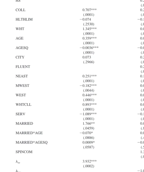
Some findings are consistent across gender and type of employment. Earnings tend to increase with education. Health limitations tend to have a negative impact on earnings, whereas living in an urban location tends to raise earnings. Workers in service occupations tend to have the lowest earnings, ceteris paribus.
Other findings vary by gender and/or type of employment. For example, among wage-and-salary workers, those living in the south tend to have the lowest earnings, ceteris paribus. The same cannot be said of employed workers; indeed, for self-employed workers, the impact of regional location varies by gender.
In many cases where findings vary across the four types of workers studied, self-employed women stand out as uniquely different. Being White and being married tend to have negative impacts on the earnings of self-employed women, whereas they have positive impacts on the earnings of the three other groups of workers studied. Also, although aging tends to enhance the earnings of the three other types of workers, it erodes the earnings of self-employed women. These patterns may reflect differences in the length of workweek and/or workyear worked by self-employed women (within the ranges defined as full-time and full-year), by race, marital status and age, and the subsequent impacts on annual earnings. Alternatively, they may reflect the presence of greater constraints and/or discriminatory elements faced by self-employed women.19
One of the most intriguing differences in the findings across the four types of workers is perhaps the most subtle: the signs of the coefficients of the selectivity variables,seand ws, are opposite by gender. For men, the findings suggest that the sorting between
wage-and-salary employment and self-employment is consistent with positive selectivi-ty.20 Rees and Shah (1986) interpreted dual positive selectivity as each group having a comparative advantage in its chosen employment.
18In an effort to check for significant gender differences, men and women were pooled into a single sample
for subsequent estimation. A dummy variable for gender was created, as were interaction terms of this dummy variable and all other X variables. Significant interaction terms in a probit estimation using the pooled data pinpointed significant gender differences in the coefficients in the probit equations for men and women. The variables found to be significant at the 10% level were: HS, CITY, NEAST, MWEST, WEST, SERV, and SPINCOM.
19In the estimation of a full specification of the self-employment earnings equation, for a pooled sample of
self-employed men and women, gender differences were found to be significant for the coefficients ofse,WHT,
AGE, AGESQ, CITY, WEST, WHTCLL, MARRIED, MARRIED*AGE, MARRIED*AGESQ, and SPINCOM, at the 10% level. In the estimation of a full specification of the wage-and-salary earnings equation, for a pooled sample of men and women employed in the wage-and-salary sector, gender differences were found to be significant for the coefficients ofws,COLL, HLTHLIM, AGE, AGESQ, CITY, FLUENT, MWEST, WEST,
WHTCLL, SERV, MARRIED, MARRIED*AGE, MARRIED*AGESQ, and SPINCOM, at the 5% and 10% levels.
20The product of the coefficient and the selectivity variable reflects the expected value of the error term in
the earnings equation, given the self-selected sample. Sincese⬎0 andws⬍0, the products of the observed
coefficients and the respective variables are positive. That is, the expected values of the error terms in each equation, conditioned on the sample, are greater than zero, making them greater for the individuals who have selected into the type of employment than for those who have not.
Table 5. OLS Estimation of Earnings Equations: Full-time, Full-year, Nonagricultural Male
Workersa
Variable Self-Employed Coefficient Wage-and-Salary Coefficient
INTERCEPT ⫺7.324* 7.889*** (.0864) (.0001) HS 0.216*** (.0001) COLL 0.707*** 0.252*** (.0001) (.0001) HLTHLIM ⫺0.074 ⫺0.148*** (.2530) (.0001) WHT 1.345*** 0.079*** (.0001) (.0001) AGE 0.359*** 0.057*** (.0001) (.0001) AGESQ ⫺0.0036*** ⫺0.0006*** (.0001) (.0001) CITY 0.073 0.215*** (.2966) (.0001) FLUENT 0.287*** (.0001) NEAST 0.251*** 0.113*** (.0001) (.0001) MWEST ⫺0.182*** 0.077*** (.0044) (.0001) WEST 0.446*** 0.058*** (.0001) (.0001) WHTCLL 0.893*** 0.057*** (.0001) (.0001) SERV ⫺1.089*** ⫺0.112*** (.0001) (.0001) MARRIED 1.766** 0.018 (.0459) (.8336) MARRIED*AGE ⫺0.070* 0.004 (.0886) (.4203) MARRIED*AGESQ 0.0009* ⫺0.00003 (.0587) (.5702) SPINCOM 1.38/106*** (.0099) se 3.932*** (.0002) ws ⫺1.089*** (.0001) F statistic 60.97*** 868.9*** (.0001) (.0001) R-square 0.186 0.315 Number of observations 4,025 33,990
ap-values are in parentheses.
Table 6. OLS Estimation of Earnings Equations: Full-time, Full-year, Nonagricultural Female
Workersa
Variable Self-Employed Coefficient Wage-and-Salary Coefficient
INTERCEPT 20.947*** 7.627*** (.0001) (.0001) HS 0.195*** (.0001) COLL 0.286*** 0.352*** (.0006) (.0001) HLTHLIM ⫺0.105 ⫺0.071*** (.3965) (.0001) WHT ⫺0.627** 0.073*** (.0407) (.0001) AGE ⫺0.203*** 0.075*** (.0056) (.0001) AGESQ 0.0020*** ⫺0.0008*** (.0085) (.0001) CITY 0.753*** 0.168*** (.0001) (.0001) FLUENT 0.351 0.145*** (.1430) (.0001) NEAST 0.251*** 0.105*** (.0090) (.0001) MWEST ⫺0.196** 0.031*** (.0326) (.0001) WEST ⫺0.300 0.150*** (.1274) (.0001) WHTCLL ⫺0.284 0.142*** (.2954) (.0001) SERV ⫺2.582*** 0.018 (.0042) (.5724) DKIDS ⫺0.175** ⫺0.059*** (.0147) (.0001) MARRIED ⫺4.143*** 0.423*** (.0001) (.0001) MARRIED*AGE 0.188*** ⫺0.029*** (.0004) (.0001) MARRIED*AGESQ ⫺0.0022*** 0.0003*** (.0006) (.0001) SPINCOM ⫺1.07/105** 4.56/106*** (.0404) (.0001) se ⫺2.840** (.0123) ws 1.159*** (.0001) F statistic 24.07*** 582.45*** (.0001) (.0001) R-square 0.242 0.305 Number of observations 1,377 25,290
ap-values are in parentheses.
For women, however, the sorting between wage-and-salary employment and self-employment reflects negative selectivity.21 In finding negative selection into self-employment among Hispanics and Asians, Borjas and Bronars (1989) argued it to be consistent with the existence of consumer discrimination, which reduces the gains from self-employment for the most able members of a minority group.
To explore these findings further, the estimated equations are used to predict wage-and-salary earnings, self-employment incomes, and probabilities of self-employment, for the given samples of workers, by gender. For purposes of comparison, the equations estimated for males are also applied to females. The mean predicted values are shown in Table 7.22
These calculations reiterate the gender differences in earnings, by type of worker, found in Tables 2 and 3: the gender gap in predicted earnings of workers in their chosen work is greater in self-employment (9.426 vs. 10.297) than in wage-and-salary employ-ment (9.823 vs. 10.265). This result is consistent with Moore (1983a).
21Blau (1985) reasoned that negative selection into farm self-employment in Malaysia tended to support the
hypothesis of a noncompetitive labor market in a developing country.
22To calculate the probabilities, the sample mean value ofis calculated. This value is then used to evaluate
1-F(), yielding the probability of self-employment for an individual with that sample mean value of
Table 7. Mean Predicted Earnings and Probabilities of Self-Employment
Self-Employment Incomea Potential Wage-and-Salary Incomea Probability of Self-Employment Self-Employed Males 10.297 10.396 .1214 95% CI (10.283, 10.310) (10.386, 10.405) 99% CI (10.279, 10.314) (10.383, 10.408) Females 9.426 9.793 .0725 95% CI (9.398, 9.455) (9.775, 9.812) 99% CI (9.389, 9.463) (9.769, 9.818) Femalesb 10.113 10.295 .0997 95% CI (10.091, 10.135) (10.277, 10.313) 99% CI (10.083, 10.142) (10.271, 10.319) Wage-and-Salary Incomea Potential Self-Employment Incomea Probability of Self-Employment Wage-and-Salary Males 10.265 10.152 .0935 95% CI (10.261, 10.269) (10.148, 10.157) 99% CI (10.260, 10.270) (10.146, 10.158) Females 9.823 9.539 .0401 95% CI (9.819, 9.826) (9.533, 9.545) 99% CI (9.818, 9.828) (9.531, 9.547) Femalesb 10.266 10.165 .0933 95% CI (10.262, 10.270) (10.160, 10.170) 99% CI (10.162, 10.171) (10.159, 10.172)
aThe natural logarithms of earnings are reported.
bThese calculations are made using the personal characteristics of the female sample, but the equations estimated from the
Simulations of outcomes for individuals having the personal characteristics of the female samples, but the equations estimated for men, shed light on the sources of difference. For wage-and-salary workers, the gender gap essentially disappears in the simulated results (10.266 vs. 10.265). That is, differences in the structure of the equations, not in the personal characteristics, account for the gender differences in wage-and-salary earnings.23For self-employed workers, the gap is substantially, but not fully, narrowed in the simulated results (10.113 vs. 10.297); differences in the structure of the equations and in the personal characteristics of self-employed men and women contribute to the gender gap in earnings in this sector.
Table 7 also reports the mean predicted earnings of workers in the type of work not chosen. Interestingly enough, predicted wage-and-salary earnings are always higher than predicted self-employment earnings.24 This finding is understandable for workers who have chosen wage-and-salary employment: their choice is consistent with wage maximi-zation. To understand the result for workers who have chosen self-employment, one must assume that there are desirable nonwage characteristics of self-employment that make it a rational choice for these workers in the maximization of expected utility. One could argue that nonwage considerations must influence women to a greater extent; they forfeit a larger percentage of earnings in choosing self-employment than do men.25
Finally, these calculations reflect the gender differences in selectivity into self-employment. Men who choose self-employment have personal characteristics that are more highly valued in the marketplace than men who choose wage-and-salary employ-ment: the former’s earnings would be higher, on average, no matter which sector they chose (10.396 vs. 10.265, if a wage-and-salary worker; 10.297 vs. 10.152, if self-employed).26 The opposite is true for women: self-employed women have personal characteristics that are less highly valued in the marketplace than women in wage-and-salary employment (9.793 vs. 9.823, if a wage-and-wage-and-salary worker; 9.426 vs. 9.539, if self-employed).27–29
23The literature exploring gender differences among wage-and-salary workers generally suggests that
differences in personal characteristics do play a role in explaining the gender wage-gap in this sector. To measure the contribution of differences in personal characteristics accurately, however, studies rely on more detailed information on occupation, field of study in formal education, and labor market experience. In summarizing these studies, Blau and Ferber (1992) reported that differences in these personal characteristics explained 60 to 66% of the wage gap between men and women with the same education level.
24A comparison of confidence intervals for these values suggests that these differences are significant 25Previous researchers have suggested that the ease of underreporting income to avoid taxes is one attraction
of self-employment (Moore, 1983b; Blau, 1987; Yuengert, 1994). If so, this practice could account for lowered self-employment income, but would not account for the gender difference, unless one were willing to assume women more guilty of it than men.
26A comparison of confidence intervals for these values suggests that these differences are significant. 27A comparison of confidence intervals for these values suggests that the differences are significant, though
the former only weakly so.
28Self-employment has been promoted by a number of states and the federal government as a way for
individuals to exit the welfare and unemployment insurance programs. See discussion and studies cited in Fairlie and Meyer (1996). Although it is possible that this activity has affected women more than men and has contributed to these findings, it cannot be determined conclusively from the present data set.
29In the comparisons of mean predicted earnings between the two types of workers, positive (negative)
selectivity of men (women) into wage-and-salary employment is masked by the systematic differences in personal characteristics of individuals who choose wage-and-salary employment. In and of themselves, these differences in characteristics tend to reduce (increase) wage-and-salary income of men (women) in the wage-and-salary sector, making it smaller (greater) than the self-employment income of self-employed men (women).
These results are consistent with the sociological theory that low-wage workers (i.e., females) are pushed into entrepreneurship, whereas high-wage workers (i.e., males) are pulled into entrepreneurship by attractive opportunities. However, the result for women contradicts the results of Devine (1994b). Devine used a different data source, with part-time or part-year workers as well as full-time and full-year workers, a different measure of earnings and a methodology not correcting for sample selection bias. She found potential wage-and-salary hourly earnings for the average self-employed female that exceeded the potential wage-and-salary hourly earnings of her wage-and-salary counterpart. This contrast raises the possibility that the mechanisms that determine self-employment status for women differ by length of workweek and/or workyear sought. Indeed, the length of workweek and/or workyear may be jointly endogenous with the choice of sector.30Although this consideration is beyond the scope of the current analysis, it certainly indicates an area in need of further investigation.
VI. Conclusion
This investigation of full-time self-employment reveals interesting gender differences. First, there is a basic gender difference in the mechanism that guides the choice between self-employment and wage-and-salary employment for a full-time, full-year worker. Women who choose self-employment have personal characteristics that are less highly valued in the marketplace than women who choose wage-and-salary employment. The reverse is true for men.
Second, certain personal characteristics affect self-employment earnings differently for women than for men. Being White and being married tend to have negative impacts on the earnings of self-employed women, whereas they have positive impacts on the earnings of self-employed men. Also, although aging tends to enhance the earnings of self-employed men, it erodes the earnings of self-employed women. It is unclear whether the resulting gender gap in self-employment earnings is the result of different supply decisions made by women or greater constraints and/or discriminatory elements faced by women.
Third, although the self-employment earnings of both men and women fall short of their wage-and-salary income foregone, the magnitude of the shortfall is greater for women. For self-employment to be viewed as a rational unconstrained choice, there must be nonwage aspects of self-employment that justify the cost. The observed gender difference suggests that women may place a higher value on these nonwage aspects of self-employment than men do.
As the self-employment of women continues to grow, there will be an opportunity to monitor these gender differences. It remains to be seen whether the rise in female self-employment will raise the relative economic status of women or increase the male/ female earnings inequality.
References
Bates, T. 1997. Race, Self-Employment, and Upward Mobility. Baltimore: The Johns Hopkins Press. Blau, D. 1985. Self-employment and self-selection in developing country labor markets. Southern
Economic Journal 52(4):351–63.
30Devine (1994a) found that self-employed women had greater variability in usual hours worked per week,
Blau, D. 1987. A time-series analysis of self-employment in the United States. Journal of Political
Economy 95(3):445–467.
Blau, F. D., and Ferber, M. A. 1992. The Economics of Women, Men, and Work. Englewood Cliffs, NJ: Prentice–Hall.
Borjas, G., and Bronars, S. 1989. Consumer discrimination and self-employment. Journal of
Political Economy 97(3):581–605.
Coate, S., and Tennyson, S. 1992. Labor market discrimination, imperfect information and self-employment. Oxford Economic Papers 44(2):272–288.
Devine, T. 1994a. Characteristics of self-employed women in the United States. Monthly Labor
Review March:20–34.
Devine, T. 1994b. Changes in wage-and-salary returns to skill and the recent rise in female self-employment. American Economic Review 84(2):108–113.
Evans, D., and Jovanovic, B. 1989. An estimated model of entrepreneurial choice under liquidity constraints. Journal of Political Economy 97(4):808–827.
Evans, D., and Leighton, L. 1989. Some empirical aspects of entrepreneurship. American Economic
Review 79(3):519–535.
Fairlie, R., and Meyer, B. 1996. Ethnic and racial self-employment differences and possible explanations. Journal of Human Resources 31(4):757–793.
Lee, L.-F. 1978. Unionism and wage rates: A simultaneous equations model with qualitative and limited dependent variables. International Economic Review 19(2):415–433.
Maddala, G. S. (1983). Limited Dependent and Qualitative Variables in Econometrics. New York: Cambridge University Press.
Min, P. G. 1984. From white-collar occupations to small business: Korean immigrants occupational adjustment. Sociological Quarterly 25(3):333–352.
Moore, R. 1983a. Employer discrimination: Evidence from self-employed workers. Review of
Economics and Statistics 65(3):496–501.
Moore, R. 1983b. Self-employment and the incidence of the payroll tax. National Tax Journal 36(4):491–501.
Oaxaca, R. 1973. Male-female wage differentials in urban labor markets. International Economic
Review 14(3):693–709.
Rees, H., and Shah, A. 1986. An empirical analysis of self-employment in the U.K. Journal of
Applied Econometrics 1(1):95–108.
U. S. Department of Commerce, Bureau of the Census. 1993. Census of Population and Housing 1990 [United States]:Public Use Microdata Sample [Computer file].2nd
release. Washington, DC: U.S. Department of Commerce, Bureau of the Census [producer], 1993. Ann Arbor, MI: Inter-university Consortium for Political and Social Research [distributor]
Yuengert, A. 1994. Testing hypotheses of immigrant self-employment. Journal of Human