Solver Choice in the SEM: A Comparative Study of Lagrangian Relaxation vs. Mixed Integer Programming

(1)

Solver Choice in the SEM:

A Comparative Study of Lagrangian

Relaxation vs. Mixed Integer

(2)

Contents

1 Executive Summary ... 3

2 Study Overview ... 5

3 A Comparison of the MIP Timeout Settings ... 14

4 MSP Production Costs ... 32

5 Consumer Costs ... 46

6 System Marginal Price ... 55

7 Commitment of Generators ... 71

8 Energy Limited Generators ... 94

9 Constraint Costs ... 102

10 MSP Software Internal Parameters ... 116

(3)

1

Executive Summary

The SEM is the wholesale electricity market covering the island of Ireland and has been operational since November 1st 2007. The market was designed as a centrally dispatched Gross Mandatory Pool model with a single System Marginal. Because the design is centrally dispatched, this requires the use of Unit Commitment software which must optimise the available generation portfolio to achieve the best economic dispatch of generators, working with the objective of minimising generator production costs in the market.

To solve unit commitment problems in power systems and markets, sophisticated mathematical optimisation software is used to determine the least cost production schedule. This software is largely seen as “black box” technology where commercial and technical data of participating generators is input and market schedules and prices are output. There are many optimisation techniques available; however, because of the non-convex nature of the unit commitment problem, more sophisticated methods are required.

Optimisation science was developed during the 1940s and 1950s using Linear Programming to solve convex problems but this could not be easily applied to unit commitment problems. The Lagrangian Relaxation (LR) method, which is now commonly applied to unit commitment problems, was first successfully developed in 1970. This has become the most commonly used technique for unit commitment in electricity markets around the world. Mixed Integer Programming (MIP) was also developed around this time but, due to computational requirements of this approach, its application was largely limited to academic circles. It has only been in the last ten years that improvements in computer processing power and memory have meant that MIP has become viable for use in commercial markets. During the development of the Central Market Systems for use in the SEM, the MSP software was designed with the option of using either an LR or MIP solver. At that time, because LR was still considered the most reliable commercial standard solver this was selected for use in the SEM; however, the MIP solver was also included and retained for use as a back up.

On a number of occasions during the first months of the SEM, due to issues with the outputs of the LR solver, SEMO made use of the back up solver for determining the Market Schedules and System Marginal Prices. Participants were made aware of SEMO’s limited use of the MIP solver when it was discussed during presentations in relation to the Dual Rated modification (Mod 34_08). After this, SEMO hosted a MOST (Market Operator Single Topic meeting) in August 2008. The purpose of this was to explain to Participants the high-level workings of the solvers and the process adopted by SEMO around the use of MIP in the SEM.

SEMO undertook to complete a comparative study of the two solvers. This report represents the results of that study. The intent of this study is to provide comparative analysis to Participants in the SEM and the Regulatory Authorities. It is hoped that this would provide assurance to Participants with regard to the issue of solver choice in the SEM and may inform future decisions and developments in this area.

A total of 154 Ex-Post Initial study cases and 16 Ex-Ante study cases were completed for this study. In each case, the original base case from SEM operations was used as a starting point but to ensure consistency of comparison, the latest version of the software was used. This means that the study cases completed with the LR program used later versions than that used in SEM operations and reviewers may note that the LR solutions used in this study differ from historical data published in the SEM.

Timeout settings were used on the MIP program where its execution would be terminated after five minutes, ten minutes and thirty minutes as appropriate.

We published a scope document1 detailing the proposed areas for review which consisted of

(4)

MSP Production Costs, System Marginal Price,

Revenue (Generator revenue and Consumer Costs),

Scheduling of Energy Limited Generators (Hydro stations), Unit commitment relative to fuel and station technology type, and Constraint Payments.

During the course of the study, we extended the scope to cover Timeout settings of the MIP solver, and

Internal software parameters.

A key observation, which is apparent, not just from the studies we completed but also from academic literature that we reviewed, is that using MIP does not provide a global optimal solution to the SEM. This is because the use of timeout settings and a convergence tolerance will always steer the MIP solver to terminate after a given parameter has been achieved (either the time or the MIP gap) thus leading to premature convergence. As a result, we must be clear that we are always comparing sub-optimal solutions.

We noted that the MIP solver produced good solutions and, in over 83% of study cases, the MSP Production Costs were observed to be lower than in the results from the LR. A key observation when reviewing the changes in the unit commitment outputs was the increased use of Energy Limited or Hydro stations. Using the MIP solver, we observed that full Energy Limits were more frequently used with significantly higher quantities of their Energy Limit being scheduled whereas this was not the case with respect to the LR results. Other fuel and station technology types did not appear to be impacted by the solver choice.

When we reviewed System Marginal Prices and Consumer Costs, we noted that the MIP solver produced higher results in over 57% of cases. This was despite an observed reduction in peak prices. Constraint Costs were also observed to increase in our study cases; however, as the Dispatch Production Cost is a static value across all studies, when one solver reduces the MSP Production Cost this will lead to increases of this nature.

Detailed observations can roughly be summed up as follows -

Using MIP over LR will more frequently lead to reduced MSP Production Costs;

Using MIP over LR has been observed to make better use of Energy Limited Generators; Using MIP with the five minute timeout setting provides best return;

MIP schedules more frequently produced higher System Marginal Prices; MIP schedules more frequently produced higher Consumer Costs; MIP schedules more frequently produced higher Constraint Costs;

Taking account that the objective of the MSP software is to minimise the aggregate MSP Production Costs across the Optimisation Time Horizon, this would mean that the MIP solver appears to better implement the requirements of the Trading & Settlement Code; however, consideration should be given to our observations with regard to increasing Consumer Costs. The mathematical function does not refer to the calculation of System Marginal Price, which is completed by separate phases of the MSP software. Therefore, minimising the MSP Production Costs by producing a more efficient unit commitment will not directly affect the calculation of the System Marginal Price and the ensuing Consumer Costs. As such, we cannot state that the MIP solver will increase the System Marginal Price but we observe that, in our study cases that it did.

However, it needs to be recognised that because of the nature of optimisation science, it cannot be guaranteed that one solver will always perform better than the other will.

We should also highlight the key finding that the LR solutions are very good relative to the sub-optimal solutions found using MIP with the current timeout and convergence tolerance settings.

(5)

2

Study Overview

2.1

Introduction

The SEM was developed as an all-island market for electricity for the island of Ireland. The design is of a centrally dispatched Gross Mandatory Pool model with a single System Marginal Price paid and charged to all Participants in the SEM. Central Unit Commitment is a key component of the design. This means that the market must optimise the available generation portfolio to achieve the best economic dispatch of generators, working with the objective of minimising generator production costs in the market. The implementation of this in the Central Market Systems is with a three-stage process in the Market Scheduling and Pricing (MSP) software –

Unit Commitment, Economic Dispatch, and Price Calculation.

To solve unit commitment problems in power systems and markets, sophisticated mathematical optimisation software is used to determine the least cost production schedule. This software is largely seen as “black box” technology where commercial and technical data of participanting generators is input and market schedules and prices are output. There are many optimisation techniques available; however, because of the non-convex nature of the unit commitment problem (that is, the inclusion of not just the linear programming problem of solving the market based on generator output and commercial/technical data, but also the integer decision of turning a generator on or off ), more sophisticated methods are required.

Lagrangian Relaxation (or LR) has been most commonly used in electricity markets for a number of years. In Lagrangian Relaxation, the primal problem (schedule generation to minimise production costs subject to some constraints) is split into a number of smaller sub-problems. Each sub-problem is solved separately with Lagrangian multipliers applied to relax the constraints. Because of the nature of how LR works, it is well understood that it will generally produce sub-optimal solutions and not produce a global optimal solution. As a result, it is widely understood that there are likely better solutions available than the outcomes achieved using an LR solver. However, this technology is still used as a practical solver for market operations.

For a long time, an alternative method called Mixed Integer Programming (or MIP) was considered in academia to be a better optimisation model but the processing and time requirements to solve a problem using MIP were prohibitive and made this impractical for use in real-world scenarios. Recent innovations in CPU technology and improvements in the MIP algorithm (Bixby, Fenelon, Gu, Rothberg, Wunderling, 1999) have meant that it is now possible to use MIP based software for market and real time operations. PJM2 in the USA, in partnership with AREVA, have developed a MIP solution for market operations and unit commitment, which has been in commercial use since 2005. CAISO is using a MIP solution in their new market since April 2009. EirGrid and SONI TSOs operate a MIP unit commitment engine to determine operating schedules on the island of Ireland.

During the implementation of the SEM, it was decided that LR based optimisation would be employed as the primary solver for unit commitment in the market. This was largely because LR techniques were considered proven and, outside of the work that was being done by PJM, no electricity market in the world was using MIP for central unit commitment problems. However, as part of the delivery of market systems prior to the start of the SEM, the Central Market Systems vendor provided a software solution that could utilise two commercial standard market solvers. One of these is proprietary software developed

2

(6)

by ABB which solves the market using Lagrangian Relaxation. The other solver is the CPLEX implementation which uses Mixed Integer Programming. Having selected the LR option as the primary solver for the SEM, the MIP solver was retained for back-up purposes for use in the event of infeasible LR solutions and other unforseen events.

Lagrangian-Relaxation (LR) is used in the SEM as the default solver to solve unit commitment. MIP has been run if certain predefined events occur, and only published if certain predefined criteria are met, namely around extreme price events driven by established bidding patterns. Details of these requirements are set out in the document “MIP_policy_V4 0 - Use of MIP for Determination of Market Schedules”, available here3 from the SEMO website. At present, it is not practical to run both solvers and compare results for each run given the current market deadlines and system and resource constraints.

The limited use of the MIP solver in study cases was openly discussed with Participants during presentations in relation to the Dual Rated modification (Mod 34_08). In response to suggestions from the Regulatory Authorities, and to provide greater assurance to Participants, SEMO hosted a Market Operator Single Topic (MOST) meeting in August 2008. During this session, presentations were given to explain the high-level workings of the solvers and the process adopted by SEMO for the use of MIP. This covered how SEMO would assess whether a schedule should be reviewed with the MIP solver and if the publication of a solution from the MIP solver was warranted. To provide further transparency to Participants, SEMO agreed to include in its Monthly Market Operator Report a listing of all Ex-Pos Initial MSP runs where the MIP solution had been published. Market Messages are also published to the SMEO website when the published schedule has been determined using the MIP solver.

At that time, SEMO also undertook to complete a comparative study of the two solvers.4 The intent of this study is to provide comparative analysis to industry Participants and the Regulatory Authorities. It is hoped that this would provide assurance to Participants with regard to the issue of solver choice in the SEM.

The intention of this study is to provide observations on the merits of each solver and recommendations to the SEM as appropriate. It is hoped that this will provide an informed background to any consultation process with regard to changing the default solver in the SEM.

2.2

Background

In total, we examined 154 Trading Days based on Ex-Post Initial data and a further 16 Trading Days based on Ex-Ante data.

All study cases days were completed using the 1.4.11 version5 of the MSP software. The MIP software used was CPLEX 10.0

The MIP implementation includes two operator configurable settings which are a time limit and a convergence tolerance, called the MIP Gap. We choose to set the time limit to five minutes. Where this did not achieve a solution within the MIP Gap, the study case would be re-run with the time limit set to ten minutes. Where this did not achieve a solution within the MIP Gap, the study case would be re-run with the time limit set to thirty minutes. We elected not to run the MIP solver for longer periods than this as there would be no practical application of a solution determined in this way.

As we will observe, only a subset of the Trading Days had to be run with the longer time limits. In total, we completed 576 individual study cases. Considering that each study case produces a set of MSP Production Costs, Market Schedule Quantities, System Marginal Prices, Shadow Prices, as well as the further values calculated from these such as Energy Payments, Constraint Payments, Consumer Costs, this resulted in the analysis of over 8.5 million individual pieces of data.

In general, study cases were completed with the market conditions that existed on the original Trading Day. The intention of this is to come up with a measure of the consequences of the solver choice on the market outcomes. A limited number of further runs were completed for the following issues:

Altering LR ALTCOM parameters ,

3_{http://www.sem-o.com/market_publications/image.aspx?id=063edd35-221d-45b5-8632-dca2d8c0ff2b}

4_{It was originally planned that this study might take place in Q4 2008 and Q1 2009. However, issues discovered}

with the MSP Demand meant a change in priority for the SEMO, which was to analyse the MSP Demand issue and provide details of this analysis to Participants.

5_{This means that previous published market schedules were not included in this study. As each run of the LR}

program was completed with a new version of the software, this will likely give rise to different results than those originally observed in actual market operations.

(7)

Running consecutive Trading Days in blocks, Altering MIP Optimality Gap, and

Amending commercial offer data for Hydro generators.

The inputs and outputs of each run of the MSP software were exported as CSV files for analysis. Most of the initial work was completed using Microsoft Access. After considerable number crunching had been completed using these tools, data was exported to Microsoft Excel. At this point, averages, trends and other points of interest were reviewed and data was further refined for inclusion in this report.

Our analysis takes the form of observing general trends in the solutions by reviewing averages, totals and standard deviations. When trying to measure the results from one solver to the next, we have done frequency analysis of these results to make observations and draw conclusions where appropriate.

In the final report, we have broken our analysis into the following areas – A comparison of the MIP timeout settings;

Productions costs;

Consumer Costs and Generator Revenues; System Marginal Prices;

Commitment of generators;

Scheduling of Energy Limited Generators; Constraint Payments; and

MSP Software internal parameters.

Each of these is presented as a separate section that can be reviewed in isolation. Each section is made up of an introduction to summarise why this specific area was focused on, an Executive Summary, a background section to provide further detail on the issue and the analysis approach, a review of the findings of the analysis and final conclusions. Appendices for the report are maintained separately. While each section can be reviewed in isolation, there is overlap between them. This Summary Overview section intends to provide an encompassing review of the findings.

2.3

Results and Review

The Unit Commitment problem is solved using complex optimisation software. In principle, the software takes the technical and commercial offer data for each generator in the SEM and uses this to determine a set of MSP Production Costs for feasible solutions. Considering the number of generators in the market and the number of pieces of input data, this produces a vast number of candidate solutions. The job of the optimisation software is to find the lowest cost feasible solution. This is done by stepping through a search space and testing the quality of each solution. Because of the non-convex nature of commercial offer data used in the SEM, this can lead to a search space where there may be several local minimum solutions. This is known as a multi-modal search space.

(8)

Some bidding patterns also add further complexity to the search space where they cause the area to become rugged; that is, the gradients in the search space become steeper and it becomes more difficult for the optimisation engine to find the best optimum solution. This was previously discussed at the SEMO MOST on the Lagrangian Relaxation and Mixed Integer Programming Solvers, held in August 2008.

Figure 2 - Multimodal search space displaying ruggedness

These elements have led to premature convergence when using the LR program when the solvers produce solutions that are sub-optimal, based on selection of a local optimal and not the global optimal solution. As we noted above, because of the nature of how LR works, it is widely understood that the solutions produced will most probably be sub-optimal solutions and this approach is not likely to produce a global optimal solution. The MIP method is considered a way to achieve a global optimal solution. However, this is only the case when MIP is run to complete convergence, which is not the case in the SEM or energy markets in general.

The MIP solver has a number of distinct phases. First of these is to solve a relaxed version of the problem. This is completed to get the lower bound on the overall solution. The Optimality Gap is calculated as the percentage variance between the best current solution and the best lower bound from this phase. The program then enters the Branch and Bound phases where it eliminates regions of the search space where the optimal solution cannot be found. This method will solve any problem to a global optimal solution but not in time limits that are practical for market operations.

The practice of applying timeout settings and convergence tolerances (or Optimality Gap limits) to MIP algorithms is quite common and is used in the SEM6 as well as PJM (Streiffret, Philbrick, Ott, 2005). This is because, despite the improvments in MIP performance over recent years, allowing the solver to seach for a true global optimal solution is still not practical for real time operations of either markets or systems (Sioshansi, 2008). As a result, while we have a measure of how close the MIP solution is to the lower bound, and can therefore estimate how close the solution is to the true global optimal, at no point does the MIP solver produce a global optimal solution.

Therefore, we have to be keenly aware that in comparing the outputs of LR to the outputs of MIP, we are comparing two sub-optimal solutions. Both are imperfect and here we attempt to measure the quality of the solutions based on this fact.

One of our first reviews was with regard to the different timeout settings that could be used with the MIP solver. Of the 154 study cases completed based on the Ex-Post Initial days, over 100 solved to within the convergence tolerance within the five minute setting. As a result, only a third of cases needed to be completed with extended timeout limits. Of these, we noted that only 50% ever solved to within the

6

(9)

convergence tolerance and to achieve that, most had to be run for thirty minutes. We observed that the best improvements in terms of convergence was from a five minute run which stopped with a MIP gap of 1.56% which improved to 0.21% when run with the thirty minute setting; however, the solver took over 16 minutes to reach this solution. The quickest resolution when set at the thirty minute level was in just over eleven minutes. The average solution time of runs that achieved the convergence tolerance was 20.33 minutes.

We observed little extra value in the ten minute setting as only six out of the study cases that did not solve with the five minute setting achieved the convergence tolerance within ten minutes.

This thirty minute timeout setting was largely used for demonstration purposes only to see if the MIP solver could produce better results with the addition of more time. It was never a consideration that running the solver for thirty minutes would be practical in terms of daily market operations. Taking account of the tight timescales under which the SEM currently operates and that the LR solution currently in use produces solutions within one minute, this would represent a significant change to operational processes if these timings were to be considered.

In general, we noted that the longer running time improved the solutions, with MSP Production Costs specifically being reduced in almost all cases7. We also noted System Marginal Prices and Consumer Costs appeared to reduce with the longer runs but by less significant amounts than the MSP Production Cost improvement. Constraint Costs were largely unaffected in this question.

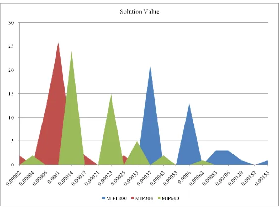
We took the findings and tried to see if there was a quality measure we could apply to the solutions. We approached this as taking the MSP Production Costs, Optimality Gap and solution time as the primary measures being as they are tied to the obligations SEMO must meet. Using the values returned from the study runs, we derived a “Solution Value”8_{. We then completed a frequency analysis of this “Solution} Value” shown below.

Figure 3 - Solution value.

The graph above shows that taking these three key inputs the MIP300 appears to have the best value for operations in the SEM. We draw the conclusion and make the recommendation that for future SEM operations where the MIP solver is run that it is run using the 300 second timeout only.

We also adopted this for the broader study on the comparison between the MIP and LR solvers and, for

7_{In general, the longer run time will result in a better solution. However, this is not always true especially when the}

MIP engine is stopped by the time limit. In this situation, the solution may vary at different runs depending on the CPU loading at each specific run. Also, the final polishing step of the algorithm may give a slightly different solution depending on the position of the best available solution in the entire search tree.

8_{This was calculated by taking the solution time in minutes, dividing by the Production Costs, and then again by the}

(10)

the other areas of interest covered in this report, we exclusively use the results of the MIP300 runs for these comparisons.

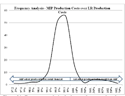
With respect to MSP Production Costs, the results observed were very interesting. While the MIP solver performed better than the LR solver in most study cases, the quality of the solutions from the LR solver appeared to be quite high. MIP produced schedules with cheaper MSP Production Costs in over 83% of the study cases, while the LR solutions were better in the remaining. Of note, in just over 42% of the study cases where the LR solver performed better, the MIP solver had achieved its convergence tolerance. While recognising the improvement with the MIP solver, it is worth noting how close the LR solutions were. In 46.1% of study cases, there was a variance of +/-0.5% between the two solutions. In 82.46% of cases, the variance between the two was +/-1%. In two study cases, the variance between the LR and MIP solvers was 0.008%. In the cases where the MIP solver performed better than the LR, the average improvement on MSP Production Costs was only 0.59%. In only 16 of the study cases did MIP improve on the LR solution by more than 1%. Equally, when LR performed better, the average improvement was 0.88% with only 11 out of 26 study cases showing variances of more than 1%.

This shows that when dealing with sub-optimal solutions from both solvers, although the MIP solution is more frequently providing lower production cost results, the solutions from the LR solver are very good in terms of the overall objective function of minimising MSP Production Costs in the SEM

From the findings, we conclude that although MIP produces solutions with lower MSP Production Costs, the improvement over those observed using the LR solver is not as significant as many people may have previously been considered. On the evidence of this study, the MIP solver generally finds better sub-optimal solutions.

This would therefore deliver the obligation of the SEM rules, to minimise the aggregate MSP Production Costs, more consistently and efficiently than the LR solver. However, the analysis also indicates that should the SEM continue with the LR solver, the quality of the solutions is very high and comparable to those from the MIP solver.

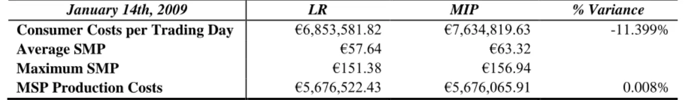
We did also note that small improvements in the Production Cost can lead to large changes in the overall SEM outcomes with significant changes to Consumer Costs being observed. Some attention is given to a study case where although the MSP Production Costs in the two solutions are within 0.008%, the variance in Consumer Costs is quite significant with costs being 11.34% higher in the outcomes of the MIP solution.

As the optimisation programs seek only to minimise MSP Production Costs, their behaviour when it comes to other issues is provided here as observations. It is not possible for us to state categorically that the use of one solver over the other will have these impacts; however, we can observe in our studies that they did. One of the principal impacts is the overall increase in System Marginal Price that we noted with the results of the MIP solver over the LR. While we should have no expectations one way or another, it could be thought that by producing a lower Production Cost the MIP solver should produce commitment decisions that result in generators from lower in the merit order being used. However, in terms of commitment decisions, we have noted that the two solvers do not vary greatly in terms of how they commit generators except that the MIP solver will commit more generators than the LR solver. As noted above, LR decomposes the problem into sub-problems to solve. In effect, the LR solver breaks the market problem down to a unit problem and solves each unit separately. Because of this, we have noted a tendency with LR solutions to be blockier with how units are scheduled; that is, the final schedules from an LR study case are more likely to be at Min Stable Generation or Max Availability. As such, the LR solver commits just enough generators to meet the System Load in this manner. The MIP solver appears to commit more generators and, in doing so, allows the Economic Dispatch phase of the problem more freedom to schedule megawatt output in a more economical way. This extra generation, while still minimising MSP Production Costs better, does affect Consumer Costs.

The most notable exception in terms of commitment decisions is with respect to Energy Limited Generator Units. This generator type, which represents the Hydro generators in the SEM, does not appear to be committed as efficiently in the LR solver. We noted in all study cases improved scheduling of Hydro generators when using MIP. Daily Hydro limits were more frequently better used in the outcomes of the MIP solver. The improvements in Hydro scheduling appear to have knock on affects in all other areas, such as in terms of the number of generators committed. By making better use of the Hydro generators, MIP does not de-commit other generator units in the same schedule and will largely keep a similar portfolio of other generation committed as the LR solver. We also note that increased used of Hydro generators has led to these generators being marginal more frequently in the MIP results. This is in

(11)

turn contributing to the increase in System Marginal Price, noted to be a result of how the Shadow Price is calculated in these circumstances.

We have also observed that LR solver has a tendency to commit a single generator unit for one Trading Period to meet a portion of the Schedule Demand when MIP will commit a combination of units. One affect of this is a larger volume of Uplift in the LR runs. However, because MIP schedules more generators especially Energy Limited generators, the overall Shadow Price in the MIP runs tends to be higher than with the LR.

Figure 4 - Average SMP, Trading Period

Figure 5 - Maximum SMP, Trading Period

Figure 6 - Minimum SMP, Trading Period

those observed when using MIP. This means that while reducing Peak Prices and Uplift, the Shadow Prices in the MIP solutions are generally higher than those in LR.

This in turn has led to more incidents of higher System Marginal Prices, and therefore Consumer Costs, in the outcomes of the MIP solver. We found that the average daily System Marginal Price increased in 57% of our study cases when reviewing the results of the MIP cases. Peak prices did reduce with a decrease of 53% in the daily maximum System Marginal Price. Uplift also appeared reduced when using the MIP solver. This aligns with the patterns observed in terms of commitment where we noted that the LR solver is more likely to incur start ups and their respective costs than the MIP solver. This appears to relate to an observed behaviour of the MIP solver where generators once started are kept on for longer periods of operation. This longer period of operation makes it more likely for the generator to recover its costs at Shadow Price rather than needing Uplift when they are shut down after shorter periods, a behaviour noted in the solutions from the LR solver.

Interesting, we observed a study case where the MIP solution, which was within the convergence tolerance, included three Shadow Prices where the price was set by the Dual Rated generator in the SEM using its oil bid step while the LR solution, though with higher Production Costs, did not have the same impact. This study case had one of the most significant variances in Consumer Costs between the two solvers where the MIP solution was 31.79% more expensive than the LR. While it may be considered that the reduction in Uplift, incidents of Peak Prices and lower daily Maximum System Marginal Prices in the outputs of the MIP solver should mean that this would produce cheaper prices, this is not the case as the daily Average shows. It can also be noted that the daily Minimum System Marginal Prices in the results of the LR solver were more frequently lower than

(12)

These changes are leading to follow on changes in the Consumer Costs of the SEM. We have observed that Consumer Costs are increasing in 57% of the study cases with an average increase of €500,000 per Trading Day. The increase in Consumer Costs also means that revenue for suppliers and generators in the SEM is also impacted. The studies completed show generator revenues increasing by around 2.5% in the solutions from the MIP solver. Though not explicitly reviewed, because the SEM is a balanced market by design, this means that supplier charges will increase by approximately the same amount. This will in turn impact on the Credit Cover requirements on Participants in the SEM.

There is no observed relationship between the Consumer Costs and other key components of this study, particularly the MSP Production Costs and the Optimality Gap in MIP. The largest single percentage increase in Consumer Costs did align with an instance where the MIP solver failed to solve to within its convergence tolerance. However, other similar instances did not show similar increases in the Consumer Costs. With one of the largest observed increases of over 30% occurring when the MIP solver stopped with an Optimality Gap of 0.8%. This is the solution noted above that contained two Peak prices from the Dual Rated generator.

While reviewing the financial impact of the two solvers, we also took into account the economic downturn that has occurred within the timeframe of the study. To try highlight where variances were being driven by the solvers from the impact of the economic climate, for much of the financial reporting, we have separated the studies into those that related to dates before the economic downturn to those that come after. To try pinpoint when this should be we reviewed the System Marginal Price in the SEM across this timeframe. This is demonstrated in the graph below.

Figure 7 - Load Weighted Average SMP

Based on this above, we selected February 2009 as boundary of the economic downturn and have reflected this in our reporting.

As noted previously, one of the most significant changes we observed related to Hydro generators and how they were scheduled by the MIP solver over the LR. While the Trading & Settlement Code sets out rules for scheduling Energy Limited Generators as being that they cannot exceed their daily limits, as these units also bid in very low costs (generally, only a small Start Up cost and zero bid cost and zero No Load Cost), it could be fairly expected that they would be low in the merit order and should be used as much as possible. The inter-temporal nature of their operation which requires that the daily limit is not exceeded across all Trading Periods does add a complexity that could led to an amount of unused energy, regardless of the solver chosen. However, the unused quantities are significantly greater in the schedules from the LR solver than from the MIP. Because these units get used to their full limit in actual dispatch, this means that compensation should come from the Constraint Payments. However, with the given commercial offer data, these payments are usually zero. We do observe the quantities by which these units are being constrained in the market. This is because while the Hydro generators are being paid a zero Constraint Payment, other thermal generators are paying back Constraints. Though this figure cannot be effectively quantified, we do consider that this will mean Constraint Payments would also increase when using the MIP solver.

(13)

In our review of Constraint Payments, we have observed that these payments more frequently increase when calculated using the outputs of the MIP solver. This is partially due to the issue of the Hydros; however, other more general commitment decisions also impact strongly on the calculation. In general, the trend appears the same using the two solvers; that is, the net daily total is either positive or negative. Trading Days which moved from negative to positive were rare and in each case, largely the result of a single commitment decision on one generator.

2.4

MSP Parameters

A modification in both LR and MIP default parameters has been carried out on a limited number of Trading Days.

This analysis has confirmed that there is limited value in modifying both the ALTCOM parameters in LR and the Optimality Gap in MIP. We have observed incidents with both where the MSP Production Costs have been improved; however, full consideration should be given to all the other aspects impacted by such changes, like SMP, Consumer Costs and Generator revenue. This has not been done in sufficient detail for this report to reach any solid conclusions, as only a limited number of study cases have been considered.

We therefore recommend that the current settings continue to be used in SEM operations and further analysis be carried out in separate studies should this be required.

2.5

Recommendations

Based on the analysis completed, we believe that the MIP program better achieves the aims of the Trading & Settlement Code with respect to MSP Production Costs. However, when we consider the other impacts in terms of System Marginal Price, Consumer Cost and Constraint Cost, we would recommend that a consultation is undertaken to allow Participants in the SEM the opportunity to digest this report and comment and suggest proposals for next steps.

(14)

3

A Comparison of the MIP Timeout Settings

3.1

Introduction

The Mixed Integer Programming solution used by SEMO has configurable timeout settings. While the program has an Optimality Gap target, defined as the MIP Gap, timeout settings are used to ensure that the program does not continue to work for periods which are operationally impractical. In the SEM, when MIP is used two timeout settings can be employed as follows:

After five minutes or MIP300 (300 seconds), and After ten minutes or MIP600 (600 seconds).

In each of these cases, if the solution found does not achieve the convergence tolerance within the set timeframe, the solver will finish and deliver the best solution found to that point, i.e. – the market solution resulting may be outside the convergence tolerance settings. For the purposes of this study, we also wanted to include an “unlimited” option. However, this was not available. In place of this, we set the timeout to 1800 seconds or 30 minutes.

In running the studies, the longer timeout settings were only used where the previous setting had timed out. As such, not all cases include runs at all settings. Before getting to the analysis of MIP against the Lagrangian Relaxation program, we will review the outputs of the various MIP runs against each other to assess if any pattern can be observed and any conclusions made. This is to determine if these can be excluded in the direct MIP to LR comparisons.

3.2

Executive Summary

A comparison of the MIP solver being run with the different timeout settings shows that while the longer runs do provide slight improvements in a number of areas, (such as better Optimality Gaps, reduced MSP Production Costs), the changes in other areas are negligible. For example, while Consumer Costs and System Marginal Prices are decreased with the longer runs, this does in turn lead to a reduction in Generator revenue, which may have separate unintended consequences in terms of encouraging investment. In addition, the changes in Consumer Costs and System Marginal Prices are not significant with the bulk of the changes occurring with the MIP1800 runs, a timeout setting that is not practical for SEM operations.

The analysis concludes that the improvements achieved by using the software with longer timeout settings do not outweigh the costs that come with the longer run time. Shorter run times are providing good quality solutions within practical timeframes for daily market operations.

It is recommended that when running the MIP solver, that the timeout setting of 300 seconds or five minutes is used – both in real operation of the SEM and through the rest of this study of MIP versus LR.

3.3

Background

To assess the results of the different MIP runs, comparative analysis has been done on the available runs under the following headings which are a subset of the criteria for analysis in the overall MIP-LR studies.

MSP Production costs, Optimality Gap,

System Marginal Prices, Consumer Costs,

(15)

Constraint Payments, and Solution times.

The Optimality Gap is a measure of how close the found solution is from the best lower bound solution determined in the first phase of the MIP program. In the SEM implementation, there is a configurable parameter called the MIP Gap, currently set at 1%. This is used as a convergence tolerance which allows the program to stop when it has achieved a solution with an Optimality Gap better than the tolerance, once time limits have not been reached.

In the study, a total of 154 “standard” Trading Days were run using the different solver options. Of these, we found the MIP300 found a solution within the MIP Gap on 105 occasions. The remaining 49 all timed out with an Optimality Gap of more than 1%. In each of these cases, the MIP600 option was run. The solver found a solution within the MIP Gap in only six of these cases. The remaining 43 were completed using the MIP1800 option.

The analysis presented in this section is based on a review of these 49 study cases.

3.4

Analysis

1.

Productions Costs

The objective function of the market solvers is to schedule Price Maker Generation, subject to some constraints while minimising MSP Production Costs across the full Optimisation Horizon. With this in mind, we have taken the measure of MSP Production Costs as being the primary measure for any analysis.

The analysis below covers the entire Optimisation Horizon and not just the Trading Day. In the SEM, this is a thirty hour period which runs from 6AM on the Trading Day to 12 noon on the following day. The Trading Day is a twenty four hour period from 6AM.

The graph below demonstrates the total MSP Production Costs, summed over the Optimization Horizon, for each of the 49 studies that were run with more than just the MIP300 option. What is noted here is that almost all studies that included extra time in the running of the solver showed reductions in the MSP Production Costs, the actual reduction in Production Cost is negligible. In some instances, the saving is so small as to be not apparent when looking at this representation.

(16)

As can be observed, the studies covered dates from 2007 through to 2009 and the notable reduction in MSP Production Costs across the studies is driven by external market drivers and not the choice of solvers, a fact that can be further observed when the MSP Production Costs are compared to the outputs of the LR solver later on. This is also shown by comparison against the average Generator Cost. This is calculated by taking the Price Quantity pairs submitted by Generators and calculating an average bid price per MW. The trend observed in the Average Generator Cost line above closely corresponds to the trend observed in the summed MSP Production Costs for the studies.

To further analyse the results, we reviewed the change between the different runs taking the MIP300 as the “base” case as this is the default setting used in production in the SEM. This was done by calculating the percentage change between the MIP300 and the MIP600 runs and between the MIP300 and the MIP1800 runs calculated as -

100 ) ( _ Pr _ ) ( _ Pr _ ) ( _ Pr _ x BASECASE Cost oduction MSP STUDYCASE Cost oduction MSP BASECASE Cost oduction MSP

The observed percentage changes are set out in Figure 8 below.

Notwithstanding one incident when the variance in Productions Costs was above +/-3% (the value of the Settlement Recalculation Threshold or SRT), across all studies the average improvement in MSP Production Costs between MIP300 and MIP600 was 0.00165%.

The average improvement between the MIP300 and the MIP1800 was 0.473%. However, between MIP300 and MIP1800 there was a higher instance of larger variances. 35 study runs were noted to have variances of more than +/-1%.

Figure 9 - Percentage Improvement in MSP Production Costs

The average monetary reduction observed between MIP300 and MIP600 was just over €7,000; while for MIP1800, the average monetary reduction we noted was €22,500.

The following graph demonstrates the results of a frequency analysis on changes in the MSP Production Costs between MIP300 and MIP600. This shows that the bulk of the changes are between +/-0.5% of the MIP300. Note the frequency value remains at zero largely between -3% and -1%.

This indicates that there is little improvement gained in the MSP Production Costs by extending the running time of the MIP solver by an extra five minutes.

(17)

Frequency analysis of percentage improvement on MIP300/MIP600

-5 0 5 10 15 20 25 30 35 40 45 -3.5 -3 -2.5 -2 -1.5 -1 -0.5 0 0.5 1

Percentage Change in MS P Production Cost

F re q u en cy o f c h an ge

Figure 10 - Frequency Analysis of changes between MIP300 and MIP600 MSP Production Costs

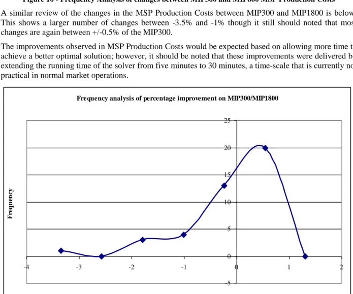
A similar review of the changes in the MSP Production Costs between MIP300 and MIP1800 is below. This shows a larger number of changes between -3.5% and -1% though it still should noted that most changes are again between +/-0.5% of the MIP300.

The improvements observed in MSP Production Costs would be expected based on allowing more time to achieve a better optimal solution; however, it should be noted that these improvements were delivered by extending the running time of the solver from five minutes to 30 minutes, a time-scale that is currently not practical in normal market operations.

Frequency analysis of percentage improvement on MIP300/MIP1800

-5 0 5 10 15 20 25 -4 -3 -2 -1 0 1 2

Percentage Change in MS P Production Cost

F re q u en cy

(18)

It should be noted that in the instances of +1% on MSP Production Costs between MIP300 and MIP1800 the MIP never solved to optimality and the Optimality Gap was better on the MIP300 and MIP600 runs than in the MIP1800 run9.

2.

Optimality Gap

The Optimality Gap is a value reported by the MSP solver. Recognising that commercial solvers rarely produce global optimal solutions and more frequently deliver the local optimal, this is a measure of how close the given solution is to the lower bound solution determined in the first relaxed phase of the problem solution. The lower the Optimality Gap, then the closer the solution is to the global optimal.

Figure 12 - Optimality Gap

Reviewing the findings summarised in the graph above, it can be observed that for the study cases which were completed using the three solver time settings, we only observed a few extreme variances in the Optimality Gap with most changes not being very significant. There are some notable exceptions such as August 25th 2009 where the Optimality Gap after the first five minute run was at 4.9%. The addition of extra time considerably improved the solution though even with a thirty minute run, this Trading Day never resolved to within the 1% MIP Gap. A similar occurrence can be noted on August 11th 2008. Again, an initial high Gap on the five minute run is improved in the thirty minute run, but still not to within the 1% MIP Gap.

Figure 13 - Average Optimality Gap

9

In general, the longer run time will result in a better solution. However, this is not always true especially when the MIP engine is stopped by the time limit. In this situation, the solution may vary at different runs depending on the CPU loading at each specific run. Also, the final refining step of the algorithm may give a slightly different solution depending on the position of the best available solution in the entire search tree.

The summary table here shows average values of Optimality Gap across the runs completed with the three time settings. As expected, the additional time does provide for improvements in the Optimality Gap, mirroring the improvements noted in Production Costs above.

However when comparing the average Optimality Gap across all MIP runs completed, this shows a different story.

(19)

Figure 14 - Average Optimality Gap, all runs

As noted above, of the 154 “standard” Trading Days that were studied, in 105 cases the MIP Gap was reached. This is 68% of the dates sampled that the MIP solver achieved optimality within five minutes or less. Running for a further five minutes only solved a further 4% of the total cases to within the MIP Gap, or 12% of those originally unresolved. Extending the solution time to thirty minutes provided solutions in a further 12% of cases, or 46% of the cases run for this duration. In total, 84% of the Trading Days studied resolved to some level of optimality. That leaves 16% that timed out without achieving an optimal solution within the 1% MIP Gap target.

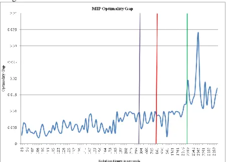
However, the improvements in the Optimality Gap are minimal with the extra time runs. With the MIP600 option, the Gap improved by an average of 0.24% over the MIP300. Running the solver for the thirty minute option only yielded a 0.7% improvement over the original MIP300. It has been observed that it is unlikely to gain any benefit from longer runs when the Gap in the MIP300 run is under 1.5%. The graph below measures the Optimality Gap against the Solution times of the runs. Without highlighting each of the separate run types, this graph shows the times of the runs that achieved an optimality gap of less than 1% – that is, where a study run for a given Trading Day did not achieve optimality within a set timeframe and had to be run again with the longer setting, these results are not included here. This graph only includes the data for study runs that completed to below the Optimality Gap or those that failed to resolve even with a 30 minute run time.

The graph lines highlight the time limits of the three run types. As can be see here, a large number of the MIP runs completed to optimality within the 300 seconds demonstrating the observations above. Allowing and additional ten minutes for a study run yields no major benefit with only a small number or additional cases resolved. Again, with the further study runs that were done over the thirty minutes timeframe only a small benefit can be observed with a large proportion of cases still not solving to within the 1% MIP Gap target.

Figure 15 - Solution time with Optimality Gap

The summary table here shows average values of Optimality Gap across all the runs. Because MIP 300 was used in all cases, its average value is the lowest here.

Here the high number of five minutes runs that achieved the Optimality Gap demonstrate the quality of MIP300 solutions when compared to the other options. This further underlines the lack of benefit that can be observed with the additional time, already noted when discussing Production Costs above.

This is especially true considering the small improvements noted by the addition of an extra five minutes running time.

(20)

As noted above, the 1800 second running time is not practical for normal market operations given the requirements of the Trading & Settlement Code. It should also be noted that of the 32% of cases that did not solve to within the 1% MIP Gap target within five minutes, 69% of these solved with MSP Production Costs that were below those of the LR runs.

3.

System Marginal Prices

A review of the System Marginal Price or SMP across the three run types demonstrated no clear pattern. As the SMP is largely the result of calculations done in the MSP software beyond the Unit Commitment phase (where the LR and MIP solvers apply) such as the Economic Dispatch and post processing phases, this was as expected. Also, the calculation of SMP is not part of the objective function that is to be solved under the Trading & Settlement Code.

However, to be fully confident we would expect to see a level of consistency between the three timeout settings. Taking a time-weighted average daily SMP, we have compared this across the 49 study runs completed with the extra timeout settings.

The results show a generally consistent pattern with similar values of average SMP across the three study run types. The graph below demonstrates the results of this comparison. It can be observed that barring two Trading Days (12th October 2008 and 22nd June 2009), the resulting SMP values are quite similar. For the two Trading Days noted with larger variances, 22nd June 2009 is one of the study cases where no solution was ever found within the Optimality Gap. However, the MSP Production Costs of the MIP300 solution were better than those of the LR study and no major improvement was found in MSP Production Costs with the longer MIP runs. The Trading Day of 12th October 2008 is one of the six cases where MIP600 improved on the original MIP300 and produced a solution within the Optimality Gap.

Figure 16 - System Marginal Price

While keeping in mind that the calculation of SMP is not part of the objective function, it is worth observing the changes that were noted. Of the 49 study cases, 25 solutions (or 51%) yielded higher daily average SMP values when run for an extra five minutes. Of the 43 study runs that were run for thirty minutes, 19 of these (or 44%) had higher daily average SMPs. The two charts below represent a frequency analysis of the changes noted in the daily average SMP.

(21)

Frequency analysis of changes to S MP between MIP300 and MIP600

-5 0 5 10 15 20 25 30 35 40 -25.00% -20.00% -15.00% -10.00% -5.00% 0.00% 5.00% 10.00% 15.00% 20.00% 25.00%

Percentage Change in S ystem Marginal Price

Figure 17 - Changes in SMP between MIP 300 and MIP 600

Frequency analysis of changes to S MP between MIP300 and MIP1800

0 5 10 15 20 25 -50.00% -40.00% -30.00% -20.00% -10.00% 0.00% 10.00% 20.00% 30.00% 40.00% Percentage Change in S MP F re q u en cy o f c h an ge

Figure 18 -Changes in SMP between MIP 300 and MIP 1800

Both these charts demonstrate that while large variances can be observed in the daily average SMP in each instance and that longer runs do appear to produce on average lower Daily SMPs, the prevailing trend is for a consistent value across all three timeout settings.

Looking at the Uplift portion of the SMP shown in figure 18 below, there is a general trend of reduction in the average daily Uplift calculation across the three run types with 63.25% of MIP600 cases and 71.4% if MIP1800 cases having smaller values of Uplift than the original MIP300 run. While taking note of this trend however, the actual monetary values of the changes noted are not always significant.

A frequency analysis of the variances, shown in figure 19 below, yields no valuable data as what can be observed as a significant percentage shift in value can be observed where little actual change in monetary terms has occurred. We have demonstrated this in the graph below where a percentage change of over 1800% can be noted. This however represents an increase of under €25 in the calculated value. Elsewhere changes of over 100% can be noted where the monetary change can be as low as €3.89.

(22)

Figure 19 - Average Uplift in SMP

Changes in calculated Uplift values between MIP300 and MIP600

-€30 -€25 -€20 -€15 -€10 -€5 €0 €5 €10 €15 €20 €25 14-N ov-07 22-F eb-0 8 01- Jun-08 09-S ep-0 8 18-D ec -08 28-M ar-09 06-Jul -09 14-O ct -09 Trade Date P er ce n tag e c h an ge ob se rve d % -2000% -1500% -1000% -500% 0% 500% € Change % Change

Figure 20 - Changes in Uplift, comparing % to € changes

As noted above, while the SMP and Uplift calculations are not part of the objective function and therefore not strictly impacted by the solver choices, the consistency of results observed here provides an assurance that there are no significant changes to results when it comes to the timeout settings of the MIP runs.

(23)

4.

Consumer Costs

Consumer Costs is considered to be the final value that the end consumer of electricity will pay. In terms of how this is calculated the general approach has been to take an approximation of payments to Generators calculated as -

SMPh

MSQuh

TPD

t in h u, Where

TPD is Trading Period Duration;

MSQuh is the Market Schedule Quantity for Generator Unit u in Trading Period h; SMPh is the System Marginal Price in Trading Period h.

the summation t in h

u,

is a summation over all Generator Units u, and across all Trading Periods h within Trading Day t

Considering that the SEM is designed as a balanced market and that the sum of all payments to Generators should be funded directly through the sum of all charges on Suppliers, this approximation is suitable though it does not consider Constraint Payments which are charged on Suppliers through the Imperfections Charge. We have separately reviewed the Constraint Payments across the different runs types to take account of this.

As the system load remained static across all the study runs completed, this means that the changes to Consumer Costs observed are driven primarily by the changes to the System Marginal Price noted above. This can be seen when comparing the summed daily Consumer Costs against the average daily SMP in figure 15 above. As these are a financial calculation that is paid and charged out according to settlement rules, this analysis was only completed across the 24 hours of the Trading Day

Figure 21 - Consumer Costs across the different MIP run types.

Equally a frequency analysis of percentage changes in the Consumer Costs shows similar trends to the same analysis on the SMP. Figure 21 below follows a similar curve to figure 16 above, reflecting that the percentage reduction in SMP does produce the expected reduction in Consumer Costs.

(24)

Frequency analysis of percentage change on MIP300/MIP600

0 5 10 15 20 25 30 35 40 -25% -20% -15% -10% -5% 0% 5% 10% 15% 20% 25%

Percentage Change in Consuner Cost

Figure 22 - Percentage Changes in Consumer Costs, MIP300 to MIP600

With the comparison of Consumer Costs between MIP30 and MIP1800 as graphed below, the shape is somewhat different.

Frequency analysis of percentage change on MIP300/MIP1800

-2 0 2 4 6 8 10 12 14 16 18 -40% -30% -20% -10% 0% 10% 20% 30% 40% 50% 60%

Percentage Change in Consumer Cost

Figure 23 - Percentage Changes in Consumer Costs, MIP 300 to MIP1800

While showing similar reductions in Consumer Costs matching the percentage decreases in SMP, there is an anomaly where the Consumer Costs increased by over 45% in the MIP1800 study run over the MIP300. This was for Trading Day June 22nd 2009 where a considerably higher SMP in the MIP1800 run produced significant variances in the Consumer Costs.

With regard to this Trading Day, no study run achieved a solution that fell within the Optimality Gap of 1%. The reported gaps were 3.06%, 2.53% and 2.38% for each of the respective runs. The MSP Production Costs for this date in the MIP1800 run were in fact higher than those in the MIP600 run even though the solution was closer to Optimality which would support some of the caution urged with regard to the quality of solutions that result when MIP algorithms are timed out (Sioshansi, 2008). It is also

(25)

noted that for this Trading Day, even the MIP300 run resolved with a lower Production Cost than the LR study.

5.

Constraint Payments

Constraint Payments are outside the main objective function of the MSP software as they represent the variance between the MSP Production Costs that Generators would incur based on the Market Schedule and the MSP Production Costs they actually incur based on how they are run in dispatch by the Transmission System Operator. The management of the Constraints costs is done by the TSO in each jurisdiction and is outside the scope of the SEM. However, the costs are collected through the Constraint Payment calculation which is defined in the SEM rules and configured in the SEMO systems. These are funded through the Imperfections Charges levied on all Suppliers in the SEM and again, collected as part of the settlement of Trading Payments and Charges in the Central Market Systems.

As this is funded by Suppliers, it can be seen as part of a grander Consumer Cost as the charges to Suppliers will inevitably be factored into retail tariffs. With this in mind, we have completed some analyses on the variances in Constraint costs between the different timeout settings of the MIP algorithm. In each case, the Constraint Payment was calculated as the Dispatch Production Cost less the Market Production Cost. The Dispatch Production Cost was calculated according to the Trading & Settlement Code based on the actual dispatch schedule of Generators on each of the relevant study days by the System Operator. As these are a financial calculation that is paid and charged out according to settlement rules, this analysis was only completed across the 24 hours of the Trading Day.

The graph below shows a comparison of total daily Constraint Payments for each of the study cases completed. While changes are noticeable, an initial review indicates that the Constraint Payments do not vary greatly across the different MIP runs.

Constraint Payments -€600,000 -€400,000 -€200,000 €0 €200,000 €400,000 €600,000 €800,000 €1,000,000 2 0 /1 2 /2 0 0 7 0 3 /0 1 /2 0 0 8 2 0 /0 1 /2 0 0 8 0 4 /0 2 /2 0 0 8 0 7 /0 2 /2 0 0 8 0 4 /0 3 /2 0 0 8 1 0 /0 3 /2 0 0 8 1 8 /0 3 /2 0 0 8 0 2 /0 4 /2 0 0 8 1 4 /0 4 /2 0 0 8 0 2 /0 6 /2 0 0 8 0 3 /0 6 /2 0 0 8 0 4 /0 6 /2 0 0 8 0 5 /0 6 /2 0 0 8 0 8 /0 6 /2 0 0 8 2 0 /0 7 /2 0 0 8 1 1 /0 8 /2 0 0 8 2 7 /0 8 /2 0 0 8 2 9 /0 8 /2 0 0 8 0 3 /0 9 /2 0 0 8 0 4 /0 9 /2 0 0 8 1 6 /0 9 /2 0 0 8 1 2 /1 0 /2 0 0 8 1 3 /1 0 /2 0 0 8 1 4 /1 0 /2 0 0 8 1 9 /1 0 /2 0 0 8 2 2 /1 0 /2 0 0 8 0 2 /1 1 /2 0 0 8 2 3 /1 1 /2 0 0 8 2 4 /1 1 /2 0 0 8 2 1 /1 2 /2 0 0 8 2 2 /1 2 /2 0 0 8 0 7 /0 1 /2 0 0 9 1 0 /0 1 /2 0 0 9 1 1 /0 1 /2 0 0 9 0 3 /0 3 /2 0 0 9 0 4 /0 3 /2 0 0 9 0 8 /0 3 /2 0 0 9 1 7 /0 4 /2 0 0 9 2 7 /0 4 /2 0 0 9 2 9 /0 4 /2 0 0 9 0 5 /0 5 /2 0 0 9 0 2 /0 6 /2 0 0 9 0 9 /0 6 /2 0 0 9 1 5 /0 6 /2 0 0 9 2 2 /0 6 /2 0 0 9 2 6 /0 7 /2 0 0 9 2 5 /0 8 /2 0 0 9

Sum of MIP300 - Total CONP Sum of MIP600 - Total CONP Sum of MIP1800 - Total CONP

Figure 24 - Constraint Payments across MIP runs

This is further borne out by the frequency analysis below completed between the MIP300 and MIP600 data. This shows a high portion of cases with little or no change in the Constraint Payment values with only exceptions where the change in value is greater than +/-10%. Note that negative changes represent a reduction in the total Constraint Payments made under a study run.

Looking at the comparison between MIP300 and MIP600 in figure 23 above, 30 study cases out of 48 reviewed showed reductions in the total Constraint Payments, while 18 study cases showing increases. However, of these 26 study cases out of the total had changes that were less than +/-1%.

(26)

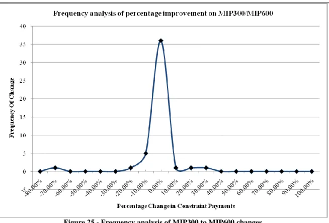
Figure 25 - Frequency analysis of MIP300 to MIP600 changes

With a comparison of the MIP600 with the MIP1800 study runs, again the bulk of the cases have only small changes though only 11 of the 42 study cases were in the +/-1% range.

In the graph below, we have excluded the Trading Day of March 18th 2008 from the frequency analysis below. This is because this Trading Day showed a change between the MIP300 and MIP1800 study runs of almost 1,500%; however, the actual monetary change between the runs was only €7,500

Figure 26 - Frequency analysis of MIP300 to MIP1800 changes

Because changes at a percentage level can be misleading, the Figures 20 and 21 below represent the frequency of the monetary changes between the MIP300 and MIP600 study cases, and between the MIP300 and the MIP1800 study cases.

Similarly to the percentage change, the indication is that large variances in the allocation of Constraint Payments are infrequent occurrences. In the comparison between MIP300 and MIP600 in Figure 20

(27)

below, 14 Trading Days of the 48 showed changes of less than €100, 32 Trading Days (including the 14 just mentioned) showed changes of less than €5,000.

There was a greater instance of monetary change in the MIP300 to MIP1800 runs demonstrated in Figure 21 below. This also showed that Constraint Payments were more frequently increasing in the longer MIP runs. We noted 11 Trading Days where the change was greater than €50,000. Of these, seven Trading Days are among those Trading Days that never solved to within the 1% Optimality Gap.

This again would be in line with academic findings that when MIP does not complete to optimality, unusual solutions can be observed.

Figure 27 - Monetary Changes in Constraint Payments, MIP300 to MIP600

(28)

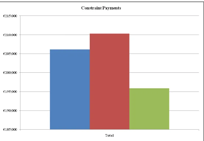
Figure 22 below shows the average Constraint Payments made across the runs in total. While the MIP1800 runs did show more frequent increases and by larger amounts than the MIP600 runs, when taken as an average across all Trading Days, Constraint Payments are lowest with the longer run. Interestingly, on average Constraint Payments made under the MIP600 run would be higher than under the MIP300.

Figure 29 - Average Constraint Payments

However, in final review, the changes to Constraint Payments under MIP between the different timeout settings are not significant. The frequency analysis above indicates that between each of the settings large changes are exceptional and in general Constraint Payments to Generators do not vary to a major extent. This indicates that the variance between how Generators are scheduled in the MIP runs with different timeout settings is not substantial.

6.

Solution times

A key consideration when reviewing the MIP options is the solution time. Taking account of the tight timelines under which the SEM operates, it is essential that the solver selected for use as the MSP software should be able to produce quality solutions in a sufficient time so that operators can ensure accuracy of outputs and meet the publication timelines obligated in the Trading & Settlement Code. While the LR program does not have specific timeout settings, the MIP program has configurable timeout settings. These are essential as with any optimisation problem, there is the potential for the program to take a considerable amount of time to reach a global optimal solution. As noted elsewhere, of the 154 study cases completed, 27 failed to solve to within 1% of optimality. Obviously, global optimal solutions exist for these study cases; however, it was not possible to find them within the time constraints we set upon ourselves when completing the study runs.

The settings of MIP300 and MIP600 are based on running the program for five and ten minutes respectively. This has been how the MIP program has been run by SEMO during other market studies and in the formulation of the SEM document, “MIP_policy_V4 0 - Use of MIP for Determination of Market Schedules”. We chose to run the program for 30 minutes as a version of an “open-ended” MIP run. This was done to assess how much longer it would take the program to produce an optimal solution and to review the quality of that solution compared to the one completed with the shorter timeout settings.

(29)

In essence, we wanted to see if study cases that had timed out at ten minutes would solve in an additional minute or two.

A 30 minute run of the program is only for study purposes and is not practical for daily operations of