OpenBU http://open.bu.edu
Theses & Dissertations Boston University Theses & Dissertations
2018
Machine learning in the real world
with multiple objectives
https://hdl.handle.net/2144/30738
COLLEGE OF ENGINEERING
Dissertation
MACHINE LEARNING IN THE REAL WORLD WITH
MULTIPLE OBJECTIVES
by
TOLGA BOLUKBASI
B.S., Middle East Technical University, 2012
Submitted in partial fulfillment of the
requirements for the degree of
Doctor of Philosophy
2018
First Reader
Venkatesh Saligrama, Ph.D.
Professor of Electrical and Computer Engineering Professor of Systems Engineering
Professor of Computer Science
Second Reader
Stanley E. Sclaroff, Ph.D. Associate Dean of the Faculty
Mathematical & Computational Sciences Professor of Computer Science
Third Reader
Brian Kulis, Ph.D.
Assistant Professor of Electrical and Computer Engineering Assistant Professor of Systems Engineering
Assistant Professor of Computer Science
Fourth Reader
Adam T. Kalai, Ph.D. Principal Researcher
Marie Curie
First, I would like to thank my advisor Venkatesh Saligrama. He gave me the op-portunity to work freely on broad range of topics. His encouragement, patience and optimism whenever I hit roadblocks in research were very valuable. I appreciate his contributions, time, ideas and funding that made my PhD experience productive and stimulating. I thank my committee members Brian Kulis and Stan Sclaroff for their feedback. When I first joined the DSML lab, I wasn’t fully ready to do research in machine learning. Joseph Wang introduced me to my first major research problem, resource-efficient learning, which turned into the focus of my first paper. He taught me how to do research, think about problems, and write papers. Collaborating with him in the earlier years of my PhD formed the foundation of my research confidence. I thank Adam Kalai in Microsoft Research Cambridge for all his mentorship and collaboration on algorithmic fairness which turned into one of the most interesting projects of my PhD. I also thank my collaborators James Zou and Kai-Wei Chang for teaching me very fundamental research principles. I thank Meng Wang for his guidance during my internship at Amazon Research, and all of Amazon Rekognition team in Seattle for a great summer and valuable real world experience. I would like to express my appreciation to Ofer Dekel for granting me the internship opportunity in his group at Microsoft Research, and continuing his collaboration afterwards.
I thank my friends on 3rd and 4th floors of the Photonics Building. Especially Onur Sahin and Jonathan Wu for all the quick meals and late night discussions on research and life. I thank Alexander Welles for always being supportive in times of need and available as a team member for little technical pursuits. I am grateful to my long time friends Cosan Caglayan, Emir Alp Yazicioglu and Selen Caner for being with me throughout life. More specifically, I would like to thank Ozan Tuncer, with whom I started the journey of engineering in undergraduate. He has been my
I thank Pricila Paulino for being a very supportive and understanding partner in long days and stressful times. I appreciate her advice, and for pushing me to live the life outside of my graduate studies.
Finally, and most importantly, I would like to thank my mother and father for being understanding and supportive throughout my PhD. Between the distance and long work hours, I haven’t had the chance to visit them as often as I would like to. Even in these circumstances, they always made themselves available with life advice and made me believe in myself.
This work was supported in part by NSF Grants CCF: 1320566, NSF Grant CNS: 1330008 NSF CCF: 1527618, the U.S. Department of Homeland Security, Science and Technology Directorate, Office of University Programs, under Grant Award 2013-ST-061-ED0001, and by ONR contract N00014-13-C-0288.
MULTIPLE OBJECTIVES
TOLGA BOLUKBASI
Boston University, College of Engineering, 2018
Major Professor: Venkatesh Saligrama, Ph.D.
Professor of Electrical and Computer Engineering
Professor of Systems Engineering
Professor of Computer Science
ABSTRACT
Machine learning (ML) is ubiquitous in many real-world applications. Existing ML systems are based on optimizing a single quality metric such as prediction ac-curacy. These metrics typically do not fully align with real-world design constraints such as computation, latency, fairness, and acquisition costs that we encounter in real-world applications. In this thesis, we develop ML methods for optimizing pre-diction accuracy while accounting for such real-world constraints. In particular, we introduce multi-objective learning in two different setups: resource-efficient prediction and algorithmic fairness in language models.
First, we focus on decreasing the test-time computational costs of prediction sys-tems. Budget constraints arise in many machine learning problems. Computational costs limit the usage of many models on small devices such as IoT or mobile phones and increase the energy consumption in cloud computing. We design systems that allow on-the-fly modification of the prediction model for each input sample. These sample-adaptive systems allow us to leverage wide variability in sample complexity where we learn policies for selecting cheap models for low complexity instances and
proach where one minimizes the system cost while preserving predictive accuracy. We demonstrate significant speed-ups in the fields of computer vision, structured prediction, natural language processing, and deep learning.
In the context of fairness, we first demonstrate that a naive application of ML methods runs the risk of amplifying social biases present in data. This danger is particularly acute for methods based on word embeddings, which are increasingly gaining importance in many natural language processing applications of ML. We show that word embeddings trained on Google News articles exhibit female/male gender stereotypes. We demonstrate that geometrically, gender bias is captured by unique directions in the word embedding vector space. To remove bias we formulate a empirical risk objective with fairness constraints to remove stereotypes from em-beddings while maintaining desired associations. Using crowd-worker evaluation as well as standard benchmarks, we empirically demonstrate that our algorithms signif-icantly reduces gender bias in embeddings, while preserving its useful properties such as the ability to cluster related concepts.
1 Introduction 1
1.1 Real-World Scenarios . . . 2
1.2 Contributions . . . 4
1.3 Organization . . . 6
2 Cost: Learning to Trade-off System Cost and Accuracy at Test-time 8 2.1 A Tree-based Policy for Cost-Accuracy Tradeoff . . . 10
2.1.1 Empirical Risk Problem . . . 12
2.1.2 Model Selection by Linear Programming . . . 15
2.1.3 Convex Risk Objective . . . 16
2.1.4 Linear Programming . . . 18
2.1.5 Experimental Setup . . . 20
2.1.6 Model Selection in Structured Learning . . . 22
2.1.7 Scene Recognition . . . 27
2.2 Structured Prediction with Resource Constraints . . . 31
2.2.1 Budgeted Structured Learning . . . 32
2.2.2 Structured Prediction Under an Expected Budget . . . 33
2.2.3 Combinatorial Search Space . . . 36
2.2.4 Anytime Structured Prediction . . . 38
2.2.5 Experiments . . . 41
2.3 Adaptive Neural Networks for Efficient Inference . . . 48
2.3.1 Adaptive Early Exit Networks . . . 51
2.3.3 Experimental Details . . . 59
2.3.4 Evaluation of Network Selection . . . 61
2.3.5 Evaluation of Network Early Exits . . . 64
2.3.6 Network Error Analysis . . . 65
2.4 Related Work . . . 67
2.4.1 Multi-Class and Black-Box . . . 67
2.4.2 Structured Prediction . . . 69
2.4.3 Deep Learning . . . 71
3 Social Constraints: Making models aware of harmful associations 73 3.1 Word Embeddings and Bias . . . 75
3.2 Discovering and Measuring Social Biases in Word Embeddings . . . . 82
3.2.1 Gender stereotypes in word embeddings . . . 83
3.2.2 Geometry of Gender and Bias . . . 87
3.2.3 Identifying the gender subspace . . . 87
3.2.4 Direct bias . . . 89
3.2.5 Indirect bias . . . 91
3.3 Removing Unwanted Social Biases from Word Embeddings . . . 92
3.3.1 Determining gender neutral words . . . 96
3.3.2 Debiasing results . . . 97
3.4 Related work . . . 100
3.4.1 Gender bias and stereotype in English . . . 100
3.4.2 Bias within algorithms . . . 101
4 Conclusions and Future Directions 103 4.1 Summary of Contributions . . . 103
4.2 Future Research Directions . . . 107
A.1 Proofs of LP-Tree . . . 109
A.1.1 Simple Tree Example . . . 109
A.1.2 Proof of Theorem A.1.1 . . . 112
A.1.3 Proof of Lemma 2.1.1 . . . 113
A.1.4 Additional Explanation of Proposition 2.1.2 . . . 114
A.2 Proofs of Resource Efficient Structured Prediction . . . 115
A.2.1 Proof of Theorem 2.2.1 . . . 115
A.2.2 Proof of Theorem 2.2.2 . . . 116
A.2.3 Proof of Theorem 2.2.3 . . . 117
A.2.4 Implementation details . . . 118
B Notes on Chapter 3 119 B.1 Generating analogies . . . 119
B.2 Learning the linear transform . . . 120
B.3 Details of gender specific words base set . . . 122
B.4 Debiasing the full w2vNEWS embedding. . . 124
B.5 Questionnaire for generating gender stereotypical words . . . 124
B.6 Questionnaire for generating gender stereotypical analogies . . . 125
B.7 Questionnaire for rating stereotypical analogies . . . 126
B.8 Analogies Generated by Word Embeddings . . . 127
References 135
Curriculum Vitae 146
2.1 Early exit performances at different accuracy/budget trade-offs for dif-ferent networks. @x denotes x loss from full model accuracy and re-ported numbers are percentage speed-ups. . . 65 3.1 The columns show the performance of the original w2vNEWS
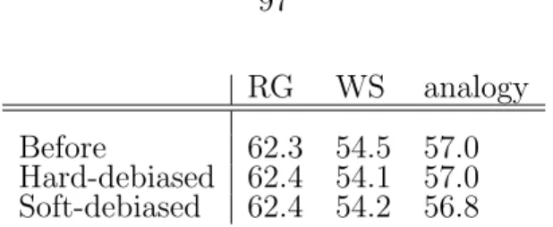
embed-ding (“before”) and the debiased w2vNEWS on the standard evalu-ation metrics measuring coherence and analogy-solving abilities: RG (Rubenstein and Goodenough, 1965), WS (Finkelstein et al., 2001), MSR-analogy (Mikolov et al., 2013c). Higher is better. The results show that the performance does not degrade after debiasing. Note that we use a subset of vocabulary in the experiments. Therefore, the performances are lower than the previously published results. . . 97 B.1 First 10 different she-he analogies generated using the parallelogram
approach and our approach, from the top 100 she-he analogies not containing gender specific words. Most of the analogies on the left seem to have little connection to gender. . . 121
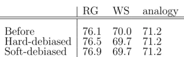
w2vNEWS embedding (“before”) and the debiased w2vNEWS on the standard evaluation metrics measuring coherence and analogy-solving abilities: RG (Rubenstein and Goodenough, 1965), WS (Finkelstein et al., 2001), MSR-analogy (Mikolov et al., 2013c). Higher is better. The results show that the performance does not degrade after debias-ing. . . 124
2·1 An illustration of our model selection tree. We have access to four models: f1, . . . f4. The models use a different combination of three
rep-resentations: rgb, hog, and gist. The system has two internal decisions nodes. g1(rgb) uses the raw pixel values to either select a low cost model
f1(rgb), medium cost modelf2(rgb, hog) or delay the decision. The last
decision node, g2(rgb, gist), acquired the gist feature selects between
predicting with available information, f3(rgb, gist), or processing hog
and predicting with the most expensive model, f4(rgb, gist, hog). The
performance of an adaptive model selection can be represented by a budget vs error curve in the upper right corner. The colors correspond to different operating points as we vary the trade off between cost and error. The overall goal is to operate close the performance of the most complex model (red) with much lower budget. The green point is an example of a desired system. . . 12 2·2 An example decision system of depth two: nodeg1(x1) selects either to
acquire feature 2 for a costc2 or 3 for a cost c3. Node g2(x1, x2) selects
either to stop and predict with features {1,2} or to acquire 3 for c3
and then terminate. Node g3(x1, x3) selects to predict with {1,3} or
with {1,2,3}. . . 14
stage cascade and a three node tree. In (b), we display the budget vs error plot for three methods: cascade and tree architecture of our LP model selection system and a DMS cascade system. While performance of LP and DMS are on par in the cascade structure, LP Tree has a significant advantage over DMS. LP tree achieves same accuracy with a significant speedup and lower computation cost(≥70% savings). . . 25 2·4 The distribution of examples that end up at 3 different stages/models
in the LP cascade at three budget operating points. . . 26 2·5 Here, we examine the histogram at .62 budget from Fig. 2·4. We
provide examples of three different words being classified at the cheapest/simplest model (frgb) and at the complex/expensive model
(frgb,hog1,hog2). As expected, more obscure and rotated words require
the complex model. . . 27 2·6 SUN Scene Categorization Results. (a) shows cascade structure used
in the experiment. In (b), we report cost savings for four accuracy levels. Loss is the difference between accuracy of the most complex model and the dynamic model at different budget points. Cost savings is the percent saved from the most expensive model. . . 28 2·7 We display example distribution among stages for scene categorization
task at different budget points. . . 28 2·8 Sample images from the railroad category sent to different models. . 29 2·9 When predicting the dependency tree, some dependencies (e.g., the
dashed edges) are easily resolved, and there is less need for expressive features in making a prediction. Our goal is to learn a system that identifies these dependencies to reduce the test-time costs. . . 33
initially incorrectly identified due to degradation in letters ”u” and ”n”. The letter classification accuracy increases after the policy acquires the HOG features at strategic positions. . . 41 2·11 Comparison of our one-shot policy (in red) with uniform strategy (in
black) and (Weiss and Taskar, 2013)’s policy for the OCR dataset. We obtained a top accuracy of 93%, which is not shown in the plots. Although the rate of accuracy gain is large for the policy that utilizes complex features, we note that policies that utilize simple features achieve lower absolute run-time in the low budget region. This is due to the overhead arising from additional inference required for complex features. . . 43 2·12 Performance of various adaptive policies for varying budget levels
(de-pendency tree accuracy vs. total execution time), is compared to a uniform strategy on word and sentence level, and myopic policy for the 23 section of PTB dataset. . . 46 2·13 Distribution of parse-tree depth for words that use cheap (green) or
expensive features (orange) for anytime policy. Time increases from left to right. Each group of columns show the distribution of depths from 0(root) to 7. The policy is concentrated on acquiring features for lower depth words. A sentence example also shows this effect. It is easy to identify parents of the adjectives and determiner. However, additional features(orange) are required for the root(verb), subject and object. . . 47
that won the ImageNet challenge over past several years. The model evaluation times increase exponentially with respect to the increase in accuracy. . . 49 2·15 An example early exit system topology (based on Alexnet). The
pol-icy chooses one of the multiple exits available to it at each stage for feedback. If the sample is easy enough, the system sends it down to exit, otherwise it sends the sample to the next layer. . . 51 2·16 An example network selection system topology for networks
Alexnet(A), GoogLeNet(G) and Resnet(R). Greenγ blocks denote the selection policy. The policy evaluates Alexnet, receives confidence feed-back and decides to jump directly to Resnet or send the sample to GoogLeNet→Resnet cascade. . . 52 2·17 Performance of network selection policy on Imagenet top-5 error. Our
full adaptive system (denoted with blue dots) significantly outperforms any individual network for almost all budget regions and is close to the performance of the oracle. The performances are reported on the validation set of ImageNet dataset. . . 60 2·18 Performance of network selection policy on Imagenet top-1 error. Our
full adaptive system (denoted with blue dots) significantly outperforms any individual network for almost all budget regions and is close to the performance of the oracle. The performances are reported on the validation set of ImageNet dataset. . . 61
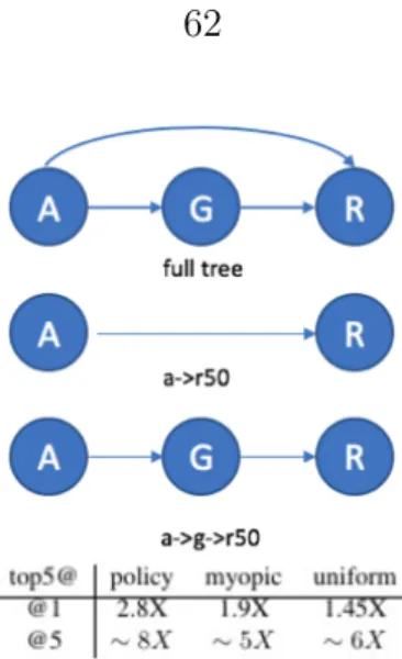
rows denote possible jumps allowed to the policy. A, G and R denote Alexnet, GoogLeNet and Resnet50, respectively. Bottom: Table com-paring the speedup of our policy versus myopic and uniform baselines at different accuracy points. . . 62 2·20 Statistics for proportion of total time spent on different networks and
proportion of samples that exit at each network. Top row is sampled at 2.0ms and bottom row is sampled at 2.8ms system evaluation . . . 63 2·21 The plots show the accuracy gains at different layers for early exits for
networks GoogLeNet (left) and Resnet50 (right). . . 65 2·22 Analysis of top-1 and top-5 errors for different networks. Majority of
the samples are easily classified by Alexnet, and only a minority of them require deeper networks. . . 66 3·1 The most extreme occupations as projected on to the she−he gender
direction on g2vNEWS. Occupations such as businesswoman, where gender is suggested by the orthography, were excluded. . . 76 3·2 Analogy examples. Examples of automatically generated analogies
for the pairshe-he using the procedure described in text. For example, the first analogy is interpreted as she:sewing :: he:carpentry in the original w2vNEWS embedding. Each automatically generated anal-ogy is evaluated by 10 crowd-workers are to whether or not it reflects gender stereotype. Top: illustrative gender stereotypic analogies au-tomatically generated from w2vNEWS, as rated by at least 5 of the 10 crowd-workers. Bottom: illustrative generated gender-appropriate analogies. . . 77
softball-football axis, which indirectly captures gender bias. For each occupation, the degree to which the association represents a gender bias is shown, as described in Section 3.2.5. . . 77 3·4 Comparing the bias of two different embeddings–the w2vNEWS and
the GloVe web-crawl embedding. In each embedding, the occupation words are projected onto the she-he direction. Each dot corresponds to one occupation word; the gender bias of occupations is highly con-sistent across embeddings (Spearman ρ= 0.81). . . 85 3·5 Ten possible word pairs to define gender, ordered by word frequency,
along with agreement with two sets of 100 words solicited from the crowd, one with definitional and and one with stereotypical gender associations. For each set of words, comprised of the most frequent 50 female and 50 male crowd suggestions, the accuracy is shown for the corresponding gender classifier based on which word is closer to a target word, e.g., the she-he classifier predicts a word is female if it is closer to she than he. With roughly 80-90% accuracy, the gender pairs predict the gender of both stereotypes and definitionally gendered words solicited from the crowd. . . 88 3·6 Left: the percentage of variance explained in the PCA of these vector
differences (each difference normalized to be a unit vector). The top component explains significantly more variance than any other. Right: for comparison, the corresponding percentages for random unit vec-tors (figure created by averaging over 1,000 draws of ten random unit vectors in 300 dimensions). . . 90
difference between the embeddings of the words he and she, and y is a direction learned in the embedding that captures gender neutrality, with gender neutral words above the line and gender specific words below the line. Our hard debiasing algorithm removes the gender pair associations for gender neutral words. In this figure, the words above the horizontal line would all be collapsed to the vertical line. . . 92 3·8 Number of stereotypical (Left) and appropriate (Right) analogies
gen-erated by wordembeddings before and after debiasing. . . 99 A·1 An example decision system of depth two: node g1(x1) selects either to
acquire feature 2 for a costc2 or 3 for a cost c3. Node g2(x1, x2) selects
either to stop and predict with features {1,2} or to acquire 3 for c3
and then terminate. Node g3(x1, x3) selects to predict with {1,3} or
with {1,2,3}. . . 109
AMT . . . Amazon Mechanical Turk CRF . . . Conditional Random Field DMS . . . Dynamic Model Selection DNN . . . Deep Neural Networks DP . . . Dependency Parsing
ERM . . . Empirical Risk Minimization HOG . . . Histogram of Oriented Gradients IL . . . Imitation Learning
LP . . . Linear Program
MDP . . . Markov Decision Process ML . . . Machine Learning
OCR . . . Optical Character Recognition POS . . . Part-of-Speech
PTB . . . Penn Treebank
RL . . . Reinforcement Learning SVM . . . Support Vector Machine WBC . . . Weighted Binary Classification
Chapter 1
Introduction
Over the last decade, we have experienced an explosion in the availability and scale of data, and access to inexpensive computational resources. This explosion has fa-cilitated the utilization of Machine Learning methods for real-world decision-making, which is increasingly impacting everyday human experience.
ML systems based on supervised learning, learn to predict by training on data. During training, ML systems optimize a loss function, `(f(X), Y) that penalizes the mismatch between predictions, f(X), and target ground-truth variables Y. Predic-tors, f(X), are trained by mapping input variables, X, such as images, text etc. to the predicted output f(X), which is then compared against the ground-truth. There are three important aspects that require further consideration in this context: (a): choosing a suitable family of predictors F that not only result in good predictions but also are easier to optimize, and generalize well with limited data; (b): Efficient methods for optimizing the loss function;(c): Construction of a suitable loss function that reflects real-world objectives and constraints. For instance, consider the task of ranking web pages with respect to their relevancy to a keyword. In this task, the true goal of the system is to learn a ranking function that orders documents that best match the keyword. The loss function must penalize poor placement of retrieved results relative to ground-truth (human annotated) rankings.
Nevertheless, in many real-world applications, we encounter additional constraints. These include fairness, computation, latency and sensor acquisition costs. For
in-stance, in our ranking web page application, our task is not only to accurately re-trieve results matching a keyword but also do so in the budgeted time (latency costs). The fundamental issue is that, it is not entirely clear as to how to augment such real-world constraints into existing learning methods. While, heuristic methods have been proposed in the literature to account for such constraints, much of this work is frag-mented. In this thesis, we propose systematic methods for learning in the context of additional constraints motivated by real-world applications.
We develop a systematic framework that allows the practitioner to explicitly model the trade-off between multiple real-world objectives.
1.1
Real-World Scenarios
In this section, we motivate our problem setup through some examples on real-world scenarios:
• You are a machine learning researcher building a software for doctors to help them diagnose certain disease types. You built a model that performs well within the quality requirements given the full set of measurements: x-ray, blood test, patient history, and ultrasound. You soon realize that doctors use which test to conduct next depending on the results on the previous ones, requiring only a subset of these tests on average. Thus, it is time consuming, expensive and extra burden on hospital’s resources to run all the tests for every patient. How can you build a system that replicates doctor’s behavior and adaptively acquires only the required features? Furthermore, a medical researcher told you that there is a large variation in the order of tests requested by different physicians for patients of similar background. Is it possible to validate the efficiency of existing feature acquisition scheme followed by physicians, and possibly discover more efficient ones?
• You are a project manager for a group of engineers that design applications for mobile phones. Your have been maintaining a project where an ML algorithm is used within a smart keyboard that predicts the next word as user inputs text. Over the course of years, you ended up with more than 10 models, each is better than the previous in accuracy. You realize that each step increase in accuracy comes in the expense of computation and latency. Knowing that both responsiveness and battery consumption are important factors of customer satisfaction, is it possible to use the expensive models only when needed? Can one reduce average battery use significantly without training a new model or degrading application accuracy? Can one easily set a maximum latency limit for devices of different computational power and let the algorithm adjust with minimal loss?
• You work in a company that is building a self driving car. You are responsible for the computer vision system for automatic pedestrian detection and evasion. The regulations state that the latency of your system should be less than 10 mil-liseconds while having more than 90% detection accuracy. Your current model is within time requirement, but can only achieve 85% accuracy. Fortunately, one of your engineers found a new research paper that describes an algorithm called Super Amazing Network. You implement it and find that it achieves 95% accuracy at 11 milliseconds. You don’t want to upgrade the hardware of all the cars already sold to customers. Is it possible to easily tweak this model to satisfy the regulations?
• You are consulting for Fortune 500 bank that wants to use machine learning to improve their credit application process. The want to predict the likelihood of someone defaulting on their loan, and have wide variety of customer data available at their disposal. You train a model that achieves good accuracy on
their data. You used Great Language Model that is trained on Big Web Corpus to create input features. However, the bank is worried about discriminating against people of protected groups and wants to know what the algorithm bases it’s decisions on. How do you measure such social bias in your algorithm? How do you make your algorithm aware of social constraints?
• You work for a startup that is aiming to revolutionize the court system in US by developing an algorithm that predicts a criminal’s likelihood of committing another crime in future. You are excited to see that your method is very ac-curate. However, you soon realize that it is relying heavily on race and age in making predictions. Even when you remove race and age related features, the results don’t seem to change. What is the problem? How do you proceed? In all these cases, there are gaps in the machine learning literature which require the practitioners to rely on heuristic measures. In this thesis, we focus on these gaps and build frameworks to address them more formally. In the end, we hope to guide both researchers and practitioners in the right direction even in cases where the exact solution to a real world dilemma is not clear.
1.2
Contributions
We can summarize the contributions of this thesis as follows:
• We leverage wide variability in image complexity and learn adaptive model se-lection policies. Our learned policy maximizes performance under average bud-get constraints by selecting “cheap” models for low complexity instances and utilizing descriptive (expensive) models only for complex ones. During train-ing, we assume access to a set of models that utilize features of different costs and types. We consider a binary tree architecture where each leaf corresponds
to a different model. Internal decision nodes adaptively guide model-selection process along paths of a tree to a leaf. The learning problem can be posed as an empirical risk minimization over training data with a non-convex multi-linear objective function. Using hinge loss surrogates we show that adaptive model selection reduces to a linear program thus realizing substantial compu-tational efficiencies and guaranteed convergence properties. Our LP approach realizes substantial computational-savings (≥70%) to achieve similar accuracy over state-of-art methods for structured prediction of words from handwritten images. We also apply our algorithm for scene categorization using crowd-sourced data and demonstrate cost-savings there as well.
• We study the problem of structured prediction under test-time budget con-straints. We propose a novel approach applicable to a wide range of structured prediction problems in computer vision and natural language processing. Our approach seeks to adaptively generate computationally costly features during test-time in order to reduce the computational cost of prediction while maintain-ing prediction performance. We show that trainmaintain-ing the adaptive feature genera-tion system can be reduced to a series of structured learning problems, resulting in efficient training using existing structured learning algorithms. This frame-work provides theoretical justification for several existing heuristic approaches found in literature. We evaluate our proposed adaptive system on two struc-tured prediction tasks, optical character recognition (OCR) and dependency parsing and show strong performance in reduction of the feature costs without degrading accuracy.
• We present an approach to adaptively utilize deep neural networks in order to reduce the evaluation time on new examples without loss of accuracy. Rather than attempting to redesign or approximate existing networks, we propose two
schemes that adaptively utilize networks. We first pose an adaptive network evaluation scheme, where we learn a system to adaptively choose the compo-nents of a deep network to be evaluated for each example. By allowing examples correctly classified using early layers of the system to exit, we avoid the com-putational time associated with full evaluation of the network. We extend this to learn a network selection system that adaptively selects the network to be evaluated for each example. We show that computational time can be dra-matically reduced by exploiting the fact that many examples can be correctly classified using relatively efficient networks and that complex, computationally costly networks are only necessary for a small fraction of examples. We pose a global objective for learning an adaptive early exit or network selection policy and solve it by reducing the policy learning problem to a layer-by-layer weighted binary classification problem. Empirically, these approaches yield dramatic re-ductions in computational cost, with up to a 2.8x speedup on state-of-the-art networks from the ImageNet image recognition challenge with minimal (<1%) loss of top5 accuracy.
• We propose novel scoring functions and experimental schemes to evaluate social bias in language models, more specifically, word embeddings. We propose two novel approaches to remove harmful biases and evaluate our results with human feedback from Amazon Mechanical Turk.
1.3
Organization
The rest of this thesis is organized as follows:
Chapter 2 focuses on costs of ML systems. We motivate the cost problem in more detail for multiple classification setups, explain the algorithms we developed for each case, provide empirical evidence as well as theoretical justification, and summarize
the related literature. Chapter 3 deals with the hidden social constraints for ML systems. We describe socially motivated constraints, propose ways to quantify them, and formulate ways to balance the accuracy, while respecting these constraints. In Chapter 4, we present concluding remarks and possible future directions. Finally, in the Appendix, we present proofs and additional details of experiments conducted in this thesis.
Chapter 2
Cost: Learning to Trade-off System Cost
and Accuracy at Test-time
In this chapter, we focus on the aspect of cost in designing machine learning systems. In real world settings, companies usually operate with constraints on cost, and there is an inherent trade-off between accuracy and resources. Assume that an engineer came up with a classifier that is marginally more accurate than another in categorizing user images into folders, but requires 10 times the computation power of previous one. The new classifier may be significantly worse in practice although it is more accurate. This is because the company may have to pay 10 times in cloud computing costs that may decrease the profits without tangible positive user experience. This better classifier may actually cause worse user experience if it is running on a mobile device, draining the battery significantly faster. In general, better accuracy comes at the cost of more resources. There are multiple sources that cause the costs to increase. First, there is a cost of acquiring the input features, this type of cost is external to the classifier. Second, there are costs associated with the algorithm itself. It is common that more complex representations require more computation. In our image categorization example, feature cost can be the cost of transferring an image through network. Hence, a lower resolution image would incur lower cost. At this point, the complexity of choosing the best classifier for our application is becoming clear.
and precise decisions on the trade-off between test-time cost and accuracy for their classifiers. We refer to this learning problem asresource-efficient learning orbudgeted learning. We will refer to the decision making system as policy throughout this chapter. We first set up the problem on black-box classifiers in Section 2.1, design an algorithm in the form of integer programming and reduce it exactly to a convex linear program. In Section 2.2, we focus on the special case of structured prediction where we exploit the classifier structure. We first modify the structured loss to introduce cost in the framework of empirical risk minimization. Later we show that the policy takes the form of structured predictor itself for certain classes of problems. We show that optimizing cost and accuracy in the case of structured prediction is computationally exponential in nature and propose approximations that work well in practice. We continue with Section 2.3 where we develop a policy specifically designed for deep neural networks. Again, we make use of the internal structure of the classifier, deep neural networks in this case, and modify it to allow joint optimization of cost and accuracy. Finally, we conclude with how our methods compare to the existing literature.
We motivate each problem within its section to make their practical use cases clear. The works presented in this chapter are published in papers: Model Selection by Linear Programming (Wang et al., 2014), Resource Constrained Structured Predic-tion (Bolukbasi et al., 2017a) and Adaptive Neural Networks for Efficient Inference
2.1
A Tree-based Policy for Cost-Accuracy Tradeoff
Image recognition often relies on expensive intermediate visual processing tasks that can hinder test-time applicability. In automated systems, low-level representations (e.g., histograms of oriented gradients) typically incur a high computation cost and impact test time tractability. In crowd-sourced systems, humans are paid to identify intermediate visual cues/attributes and can be prohibitively expensive for test-time. On the other hand, we can leverage the fact that images exhibit wide diversity in complexity. Indeed, recognition for many typical instances can be performed to desired accuracy with relatively cheap models that utilize computationally inexpen-sive features or only a few expeninexpen-sive attributes. This key insight motivates our model selection policies that adapts to problem difficulty. We learn decision rules from train-ing data, which when presented with a new example selects the most informative and cost-effective model for that example.
We describe our work in the context of handwriting recognition and scene cat-egorization. In handwriting recognition, the objective is to predict a word given a sequence of letter images. While a more complex model, that uses several feature types or processing at multiple resolutions yields better predictive performance, the system suffers from the prohibitively slow computation time (Weiss et al., 2013). Scene recognition—another scenario where budget constraints arise—is a difficult task due to the large number of classes and interclass similarity (Patterson and Hays, 2012). Low-level features are often insufficient for acceptable performance; and high-level attributes crowd-sourced by Amazon Mechanical Turk (AMT) are often used in predictive models incurring monetary costs. Due to the wide diversity of images, high-cost attributes/features are often unnecessary for many images to meet accept-able performance. Indeed “cheap” models can often be used for typical cases. The goal of this work is to learn policies that adaptively utilize cost-effective models while
ensuring desired performance. If we represent an input data instance as x, its un-known response as y and our adaptive selection system as g(x) then the high level objective is to minimize the average prediction error subject to an average budgetB.
min
g E[ error(g(x), y) ] s.t. E[ cost(g(x)) ] ≤B
Several researchers have explored similar problems (Gao and Koller, 2011; Jiang et al., 2012; Karayev et al., 2012; Weiss et al., 2013) which we will describe later in detail.
The novel contribution that differentiates our work is a convex formulation for learning an adaptive model selector. We assume we are given a collection of precom-puted models. Each model operates on features with different costs. Our decision system is described by a binary tree (see Fig.2·1). Each leaf corresponds to a particu-lar model. Due to this structure, models can share features/attributes. The internal decision nodes route examples along the paths in a tree culminating in a model that is cost-effective while meeting desired accuracy levels.
Learning decision functions at each node of such a tree can be posed as an empirical risk minimization(ERM) problem that balances acquisition cost and misclassification error. We express ERM as an extremal(maxima) point of sums of indicator functions. This key transformation enables us to introduce convex surrogates for the indicator functions and, in turn, results in a convex objective. Without our transformation, direct substitution of surrogates in the original empirical risk results in a non-convex multi-linear formulation which is known to be NP-complete (Megiddo, 1988).
Next, by choosing hinge loss for upper-bounding surrogate, we reduce the objec-tive to a linear program (LP): a very well studied problem with strong convergence guarantees and efficient optimization algorithms. However, other convex surrogates are also possible, and our formulation carries all the advantage of convex programming such as repeatability, global convergence and computational efficiency. In contrast,
f
1f
2f
3f
4(
)
(
)
(
)
(
)
g
1(
)
g
2(
)
Average Budget Pr ed ic ti o n Er ro rFigure 2·1: An illustration of our model selection tree. We have access to four models: f1, . . . f4. The models use a different
combi-nation of three representations: rgb, hog, and gist. The system has two internal decisions nodes. g1(rgb) uses the raw pixel values to
ei-ther select a low cost model f1(rgb), medium cost model f2(rgb, hog)
or delay the decision. The last decision node, g2(rgb, gist), acquired
the gist feature selects between predicting with available information,
f3(rgb, gist), or processing hog and predicting with the most
expen-sive model, f4(rgb, gist, hog). The performance of an adaptive model
selection can be represented by a budget vs error curve in the upper right corner. The colors correspond to different operating points as we vary the trade off between cost and error. The overall goal is to oper-ate close the performance of the most complex model (red) with much lower budget. The green point is an example of a desired system.
alternating non-convex optimization approaches (Trapeznikov and Saligrama, 2013; Bennett and Mangasarian, 1993; Wang and Saligrama, 2012) applied to similar prob-lems do not have such guarantees.
2.1.1 Empirical Risk Problem
In a typical learning problem, a data instance, x∈ X has a corresponding response
y ∈ Y. The goal is to learn a model f(x) ∈ Y that correctly predicts the response variable y. For notational purposes we let D denote the unknown joint distribution for (x, y).
For example, in scene categorization, the objective is to predict a scene category,y, in an image x. Here, the response space Y consists of L possible classes, {1, . . . , L}. In structured prediction, the input, x, is a sequence of handwritten letter images. The goal is predict the written word. In this case,Y is a combinatorial output space consisting of all admissible letter sequences.
Each instance x is composed of M different vector-valued feature/attribute com-ponents. The mth feature component has an associated costcm. We assume we have
access to K prediction models: f1(x), . . . , fK(x) that are a priori given and fixed.
The input to each model, fk(·), is a sub-collection, Sk, of the M attributes or
fea-tures. Each model has an associated cost of prediction: P
m∈Skcm. In addition, each
model’s prediction performance is evaluated with a loss function given the ground truth response variable: L(f(x), y) ∈ R+. For instance, in classification, the loss is
simply a 0/1 error, L(f(x), y) =1[f(x)6=y].
Our goal is to learn a decision system that dynamically selects one of these models for every instance x. We represent our system as a binary tree. The binary tree is composed ofK leafs andK−1 internal nodes. At each internal node,j = 1, . . . , K−1, is a binary decision function, sign[gj(x)]∈ {+1,−1}. This function determines which
action should be taken for a given example. The binary decisions, gj(x)’s, represent
actions from the following set: stop and predict with the model that uses the current set of features or choose which feature to request next. Each leaf node,k = 1, . . . , K, corresponds to a terminal decision of predicting with the model fk(x) based on the
available information. For notational simplicity, we denote applying a decision node and a leaf model asgj(x) andfk(x) respectively. Note the functions implicitly operate
only on the feature sets that have been acquired along the associated path to each node.
g
1g
2g
3 + -- + - +f
1f
2f
3f
4 g1(x) g2(x) g3(x) " # Leaf 1 −1 −1 0 Leaf 2 −1 +1 0 Leaf 3 +1 0 −1 Leaf 4 +1 0 +1 = P z }| { 0 0 0 0 1 0 1 0 0 1 0 1 − N z }| { 1 1 0 1 0 0 0 0 1 0 0 0 Figure 2·2: An example decision system of depth two: node g1(x1)
selects either to acquire feature 2 for a cost c2 or 3 for a cost c3. Node
g2(x1, x2) selects either to stop and predict with features {1,2} or to
acquire 3 for c3 and then terminate. Node g3(x1, x3) selects to predict
with {1,3} or with {1,2,3}. system risk: R(g,x, y) = K X k=1 Rk(fk,x, y)Gk(g,x) (2.1)
Here, g = {g1, . . . gK−1} is the set of decision functions. Rk(fk,x, y) is the risk of
making a decision at a leaf k. It consists of two terms: loss of the model at the leaf and the cost of features corresponding to the sub-collection of attributes,Sk, acquired
along the path from the root node to the leaf; and α is a parameter that controls trade-off between acquisition cost and model performance.
Rk(fk,x, y) = L(fk(x), y) +α
X
m∈Sk
cm (2.2)
Gk(g,x)∈ {0,1} is a binary state variable indicating whether or not an instancexis
terminated at the kth leaf. As illustrated in Fig. 2·2 we compactly encode the path from the root to every leaf in terms of internal decisions, gj(x)’s, by two auxiliary
binary matrices: P, N ∈ {0,1}K×K−1. If P
k,j = 1 then, on the path to leaf k, a
decision node j must be positive: gj > 0. If Nk,j = 1 then on the path to leaf k, a
decision at node j must be negative: gj ≤0. Akth row in Pand Njointly encode a
path from the root node to a leaf k. The sign pattern for each path is obtained by P−N. Using this path matrix, the state variable can be defined:
Gk(g,x) = K−1
Y
j=1
[1gj(x)>0]Pk,j[1gj(x)≤0]Nk,j (2.3)
Our goal is to learn decision functions g1, . . . , gK−1 that minimize the expected
system risk:
min
g ED[R(g,x, y)] (2.4)
However, the probability distribution D is assumed to be unknown and cannot be estimated reliably due to potential high-dimensionality of attributes. Instead, we are given a set of N training examples with full features, (x1, y1), . . . ,(xN, yN). We
approximate the expected risk by a sample average over the data and construct the following empirical risk minimization (ERM) problem:
min g N X i=1 R(g,xi, yi) = N X i=1 K X k=1 risk of leafk z }| { Rk(fk,xi, yi) K−1 Y j=1 [1gj(xi)>0] Pk,j[1 gj(xi)≤0] Nk,j | {z } Gk(·) = state ofxiin a tree (2.5)
Note that by the definition of risk in Equation (2.1), the ERM problem can be viewed as a minimization over a function of indicators with respect to decisions: g1, . . . , gK−1.
2.1.2 Model Selection by Linear Programming
A popular approach to solving ERM problems is to substitute indicators with convex upper-bounding surrogates, φ(z)≥1[z] and then to minimize the resulting surrogate
in our setting. Previous attempts to solve problems of this form have focused on com-putationally costly alternating minimization approaches (Trapeznikov and Saligrama, 2013; Bennett and Mangasarian, 1993; Wang and Saligrama, 2012) with no guaran-tees on optimality. A key point of this work is that rather than attempting to solve this non-convex surrogate problem, we instead reformulate the indicator empirical risk in (2.5) as a maximization over sums of indicators before introducing convex surrogate. Our approach yields a globally convex upper-bounding surrogate of the empirical loss function.
2.1.3 Convex Risk Objective
In reformulating the risk, it is useful to define the ”savings” for an example. The sav-ings, πi
k, for an examplei, represents the difference between the worst case outcome,
Rmax and the risk Rk(fk,xi, yi) for terminating at the kth leaf. Intuitively Rmax is
the cost of incorrectly predicting with the most expensive model (the model that uses all the features):
Rmax = max y0 L(y, y 0 ) +αX m cm (2.6) πik=Rmax−Rk(fk,xi, yi) (2.7)
Note that the savings do not depend on the decisions, gj0s, that we are interested in learning.
For a binary tree, T, composed of K−1 internal nodes andK leaves, it turns out that the risk in Equation (2.5) can be rewritten as a maxima ofK terms. Each term is a weighted linear combination of indicators, and each weight corresponds to the
savings lost if the decision inside the indicator argument is true. Before stating the result, we define the weights for the linear combination in each term of the max. For an internal nodej, we denote Cjn as the set of leaf nodes in a subtree corresponding to a negative decisiongj(x)≤0. AndCjp is the set of leaf nodes in a subtree corresponding
to a positive decision. For instance in Fig. 2·1, C1p ={Leaf 3, Leaf 4}.
For a compact representation, recall that thekth rows in matricesPandNdefine a path to leaf k in terms of g1, . . . , gK−1, and a non-zero Pk,j or Nk,j indicates if
gj ≶ 0 is on the path to leaf k. So for each xi and each leaf k, we introduce two
positive weight row vectors of lengthK −1:
win,k =Nk,1 X l∈C1p πil, . . . ,Nk,K−1 X l∈CK−p 1 πil wp,ki =Pk,1 X l∈Cn 1 πli, . . . ,Pk,K−1 X l∈Cn K−1 πil (2.8)
Using these weight definitions, the empirical risk in (2.5) can be rewritten as: Lemma 2.1.1 The empirical risk of tree T is:
R(g,xi, yi) =Rmax− K X k=1 πik+ max k∈{1,...,K}w i p,k 1g1(xi)>0 .. . 1gK−1(xi)>0 +wn,ki 1g1(xi)≤0 .. . 1gK−1(xi)≤0 (2.9)
The proof of this lemma is included in the Appendix A.1.3. The jth component of wi
n,k multiplies1[gj(xi)≤0] in the term corresponding to the
kth leaf. For instance in our four leaf example in Figure 2·2, the weight multiplying
1[g1(xi)≤0] is the sum of these savings for leaves 3 and 4 (i.e. savings lost if g1 ≤ 0).
wi n,1 1 =π i 3+π4i. Therefore, setsC p
j, Cjndefine which πki’s contribute to a weight for
a decision term. If Pk,j orNk,j is zero then decisiongj ≷0 is not on the path to leaf
k and the weight is zero.
Intuitively, the empirical risk in (2.9) represents a scan over the paths to each leaf (k = 1, . . . , K), and each term in the maximization encodes a path to one of the K leaves. The active term in the maximization corresponds to the leaf to which an observation is assigned by the decision functions g1, . . . , gK−1. Additionally, the
is active. In our example, if the decision function g1(xi) is negative, leaves 3 and 4
cannot be reached by xi, and thereforeπ3i and π4i, the savings associated with leaves
3 and 4, cannot be realized and are lost.
An important observation is that each term in the max in (2.9) is a linear com-bination of indicators instead of a product as in (2.5). This transformation en-ables us to upper-bound each indicator function with a convex surrogate, φ(z):
φ[gj(x)]≥1[gj(x)>0], φ[−gj(x)]≥1[gj(x)≤0]. The result is a novel convex upper-bound
on the empirical risk in (2.9). We denote this risk as Rφ(g). And the optimization
problem over a set of training examples, {xi, yi}Ni=1 and a family of decision functions
G: min g∈G N X i=1 Rφ(g,xi, yi) (2.10) 2.1.4 Linear Programming
There are many valid choices for the surrogateφ(z). However, if a hinge loss is used as an upper bound andGis a family of linear functions of the data then the optimization problem in (2.10) becomes a linear program (LP).
Proposition 2.1.2 For φ(z) = max(1−z,0) and linear decision functions
g1, . . . , gK−1, the minimization in (2.10) is equivalent to the following linear program:
min g1,...,gK−1,γ1,...,γN α1 1,...,αNK−1,β11,...,βK−N 1 N X i=1 γi subject to: (2.11) γi ≥wip,k αi1 .. . αi K−1 +win,k β1i .. . βi K−1 , i∈[N], k ∈[K] 1 +gj(xi)≤αij, 1−gj(xi)≤βji, α i j ≥0, β i j ≥0, j ∈[K−1], i∈[N]
We introduce the variable γi for each examplex
over leaves to a set of linear constraints. Similarly, the maximization within each hinge loss is converted to a set of linear constraints. The variables αi
j upper-bound
the indicator1gj(xi)>0 and the variablesβji upper-bound the indicator1gj(xi)≤0.
Addi-tionally, the constant terms in the risk are removed for notational simplicity, as these do not effect the solution to the linear program. More details of this conversion can be found in Appendix A.1.4.
Complexity: Linear programming is a relatively well-studied problem, with ef-ficient algorithms previously developed. Specifically, for K leaves, N training points, and a maximum feature dimension ofD, we haveO(KD+KN) variables andO(KN) constraints. The state of the art primal-dual methods for LP are fast in practice, with an expected number of iterations O(√nlogn), where n is the number of variables (Anstreicher et al., 1999).
Generalization: The VC-dimension of our decision trees is small, growing on the order of Klog(K)D, where D is the maximum VC-dimension of the decision func-tions and classification funcfunc-tions (Sontag, 1998). Intuitively, the slow growth of the VC-dimension suggests that the complexity of the decision system is comparable to the complexity of each individual classifiers, f1, . . . , fK, and therefore generalization
error of the system is comparable to the generalization error of the individual classi-fiers (see (Sontag, 1998; Wang and Saligrama, 2012) for a more in-depth analysis of generalization of the system).
Kernelization: Our formulation can handle more complex decision functions g(x) by kernelization. The observations xi are replaced in the LP by ψ(xi) for some
expanded basis function ψ(·). For expanded basis functions, a natural solution is to add `2 regularization on the decision functions, converting the LP to a quadratic
program. Addition of `2 regularization removes non-unique solutions, with solution
problem (for a sufficiently small regularization parameter value). Furthermore, the
`2 regularization allows for the problem to be kernelized, as the optimization can be
expressed with respect to expanded basis inner products of the form ψ(xi)Tψ(xj) in
the dual problem. While this is possible, yielding a quadratic optimization problem in place of the proposed LP, empirical evidence indicates that on real-world data the family of linear and low-order polynomial decision functions is sufficiently rich and therefore we do not explore kernelization in the experimental section.
Algorithm 1 Model Selection by LP
INPUT:f1(x), f2(x), . . . , fK(x) .Models; S1, S2, . . . , SK . Features used by each
model; P,N .Tree structure; (x1, y1),(x2, y2), . . . ,(xN, yN) . Training Data; α .
Trade-off parameters
for (i, k) = {1, . . . , N} × {1, . . . , K} do Compute savings in (2.7): πi
k ←Rmax−Rk(fk,xi, yi)
Compute weight vectors in (2.8): win,k,wp,ki end for
Solve linear program in (2.11):
[g1(x), g2(x), . . . , gK−1(x)]←LP solver({wn,ki ,wip,k})
OUTPUT:Model Selection Tree: g(x)
2.1.5 Experimental Setup
We demonstrate our LP model selection approach in Algorithm 1 on two important prediction tasks in computer vision. First, we apply our method to the problem of structured prediction. We use the handwriting dataset for word prediction and compare our method to the reinforcement learning(RL) based model selection (Weiss et al., 2013). Here, the cost is computation time for processing Histogram of Oriented Gradients(HOG) transforms of different scales. For the second experiment, we apply our method to the SUN scene categorization (Patterson and Hays, 2012) dataset. Here instead of using image processing features, we use human generated descriptor as inputs to a classifier. In this set-up, the cost of feature acquisition is the monetary value paid to Amazon Mechanical Turk workers.
Performance Metric: Our goal is to train a set of decision functions for a fixed tree that minimizes prediction loss subject to an average budget constraint. We examine average acquisition cost vs. average prediction loss to compare performance of the proposed LP approach. We sweep over values of the trade-off parameter α in order to learn systems of varying average budget, resulting in a series of learned trees of differing prediction rates and average budgets. Increasing the value of α biases the system to learn decisions with low average acquisition cost with an increased system error, while decreasing the value α yields systems with smaller error at the expense of an increase in cost. Although a system may not be learned that exactly matches a desired budget, any point in the convex hull of budget/error points learned is achievable by weighted randomization over learned systems. As a result, we take the lower convex hull of points in the space of average error vs. average cost to learn a decision system for any average budget. Note that in the experimental results, a convex hull over the training points is taken, with the corresponding policies applied to unseen test data, and therefore the resulting curve is not necessarily a convex hull. In all experiments, we first divide the data into 10 training/test folds. Within each fold, we further divide the training data of each fold into 10 sub-folds. In these sub-folds, we use all but one sub-fold to train the models, and apply this learned predictor to estimate the losses for the unused sub-fold These sub-folds are used to more accurately represent the prediction ability of the models for learning our adaptive system.
Leaf Models: Each individual leaf model,f1, . . . , fK, operates on a subset of the
features acquired on the path to that leaf. We assumefk’s are pre-computed prior to
learning the decision system. The goal of this work is to demonstrate the advantage of an adaptive selection system therefore we do not seek to learn the most accurate models. We simply illustrate the gain in relative performance: same level of accuracy
as the most complex model achieved with lower budgets. 2.1.6 Model Selection in Structured Learning
Structured Learning Problem: In structured learning, the goal is to learn a model from a set of training samples that maps inputs x ∈ X to the outputs y ∈ Y. In a typical structured prediction setup (Tsochantaridis et al., 2005), the response space Y is not simply a discrete label but instead a more complex structured output. In particular, we focus on the problem of predicting words from handwritten characters, where the output space, Y, is a string of letters of varying length. The goal is to learn a scoring function, Ψw(x, y), over training data such that the prediction model,
f(x) = arg maxy∈YΨw(x, y) matches the given training structure.
We use a function Ψw(x, y) =w·h[x, y] which is linear in the score featuresh:X ×
Y →Rp. In general, there are exponentially many outputs and solving this inference
is computationally infeasible. However, h is usually constructed to decompose over subsets of ythat enables this problem to be solved efficiently. In our experiment, we adopted a first-order linear conditional random field(CRF) model which is commonly used in optical character recognition (OCR) tasks (Weiss et al., 2013; Maaten et al., 2011). In this model, the score features decompose into sum of unary and pairwise terms. Given an input character image sequence of x= {x(1), ..., x(l)}, the score of output sequence can be written as,
Ψw(x, y) = ` X j=1 h[x(j), y(j)]·w+ ` X j=2 h[x, y(j−1), y(j)]·w (2.12)
where y(1), ..., y(`) are labels for individual characters in the word y. Given the weight vector w, we use max-sum algorithm (Bishop, 2006) to solve the inference problem. To learn the weight vector w, we solve maximum conditional likelihood using stochastic gradient descent. We used the implementation in (Maaten et al.,
2011) for this purpose.
Note that in this section we use structured prediction in our experiments to show the flexibility of our tree decision system in the case of more complex classifiers. As seen in Algorithm 1, given pre-trained modelsfi, this method only requires the ability
to compute savings for each sample which in turn require a loss and cost feedback. Our method’s flexibility comes with some shortcomings which we will digress in Section 4. Furthermore, we will specifically focus on structured predictors in Section 2.2.
Dataset and Simulation Details: We used the OCR data set from (Taskar et al., 2003). This data set has 6,877 handwritten words where each word is rep-resented as sequence of 16x8 binary letter images. There are 55 unique words, 26 unique characters and 55,152 letters.
Following (Taskar et al., 2003), we use three sets of features: raw images, HOG (hog1) (Dalal and Triggs, 2005) computed in 3x3 bins and a finer HOG computed on 2x2 bins (hog2). We have four CRF models: frgb, frgb,hog1, frgb,hog2, frgb,hog1,hog2. The
computational cost of processing the raw images is assumed to be negligible, while the computational cost of the 2x2 and 3x3 HOG features are assumed to be equal and proportional to the length of the word.
The goal is to learn a system to minimize character recognition error subject to an average computational cost constraint per letter. We train two architectures: a two stage cascade and a three decision node binary tree as illustrated in Fig. 2·3. Note the tree allows greater flexibility by allowing us to acquire hog2 directly from rgb while a cascade has to acquire hog1 before processing hog2.
Following the framework presented in (Weiss et al., 2013), the decision functions in our LP tree also act on meta features as opposed to the raw features. These meta features reflect the fit of the structured predictor f(·) to the training set population.
predic-tions, the average of the min/max and mean entropies of the marginal distributions as predicted at each position in the word by the predictor at that stage. Additional meta-features count the number of times a 3-gram 4-gram and 5-gram are predicted but never occur in the training set.
Dynamic Model Selection baseline: We compare our approach to dynamic structured model selection method (DMS) in (Weiss et al., 2013). There the au-thors employ a cascade architecture with models arranged sequentially in the order of increasing cost, and learn a policy that controls whether an example should be predicted using the current model or rejected to the next more expensive model. For their DMS architecture, we use the same cascade as for our approach.
The authors define the value of delaying a decision as a decrease in the loss when a sample is moved from stage i to i + 1. This value function is modeled as a linear combination of the meta-features. The policy then sends the instance that suffer the maximum predicted loss reduction to the next stage until a predeter-mined budget limit is hit. The value of skipping a stage is defined as: V(fi,x,y) =
L(fi−1(x),y) −L(fi(x),y). The policy parameter β is found by ridge regression,
arg minβλ||β||22 +
P3
i=2
Pn
j=1(V(fi,xj, yj)−βTφ(xj, f1:i−1))2, where φ denotes the
meta-features for given sample and stage predictors. The test time value is then defined as J(τ1, ..., τn, η) = Pnj=1P
τj
i=2βTφ(xj, f1:i−1), where τj denotes how many
features are computed for example j. During test time, the total value is greed-ily maximized until the budget constraint B prevents any other features from being computed.
Discussion: We report average error for different values of average budget (see Fig. 2·3). For simplicity, we normalize the units to the fraction of the maximum budget allowed. For example, if the system operates at budget 1 then every example is routed to the most expensive model frgb,hog1,hog2 (the best accuracy). For budget
rgb hog1 hog2 hog2 frgb frgb,hog2 frgb,hog2 frgb,hog1 rgb hog1 hog2 frgb frgb,hog2 frgb,hog1 Tree Cascade (a) 0 0.2 0.4 0.6 0.8 1 0.11 0.12 0.13 0.14 0.15 0.16 0.17 0.18
Fraction of max budget used
Letter classification error
LP tree DMS cascade LP cascade
(b)
Figure 2·3: (a) shows two system structures used in the OCR experi-ment: a two stage cascade and a three node tree. In (b), we display the budget vs error plot for three methods: cascade and tree architecture of our LP model selection system and a DMS cascade system. While performance of LP and DMS are on par in the cascade structure, LP Tree has a significant advantage over DMS. LP tree achieves same ac-curacy with a significant speedup and lower computation cost(≥70% savings).
0, every example remains with the cheapest model, frgb. An adaptive system with a
budget between 0 and 1, utilized the cheap model for some examples and the expensive model for others resulting in a lower budget but accuracy equivalent to the expensive model.
The experiments clearly highlight the advantages of our approach. Our LP cas-cade performance matches the accuracy for all budget values of a DMS cascas-cade. How-ever, when we introduce a more flexible tree architecture instead of a cascade, the performance dramatically improves. Our LP tree exhibits significant computational-savings(≥ 70%) and speedup to achieve similar accuracy as a DMS cascade. In a
cascade, an example cannot go directly to the model, frgb,hog2 while in a tree this
decision is possible and results in higher cost efficiency. In addition, our approach learns a separate decision for every internal node in the tree allowing for more com-plex selection functions. In contrast in DMS, the same policy function is used at every stage of the cascade limiting the discriminative power of the decision system. Note that DMS does not generalize to trees in an obvious way since it is in essence an early stopping policy.
1 2 3 0 100 200 300 400 Avg word length: 8.10 Avg word length: 6.88 1 2 3 0 100 200 300 400 Avg. word length: 6.92 Avg. word length: 7.28 Avg. word length: 7.93 1 2 3 0 100 200 300 400 Avg. word length: 6.48 Avg. word length: 8.97 . .26 .62 .73 frgb frgb,hog1 frgb,hog2 @Budget
Figure 2·4: The distribution of examples that end up at 3 different stages/models in the LP cascade at three budget operating points.
In addition to the error vs budget performance, we explore the distribution of examples that are being routed to the three models in our LP cascade architecture. Figure 2·4 illustrates the analysis of systems corresponding to budgets: 0.26, 0.62 and 0.73. As expected at a budget of 0.26, model utilization is evenly distributed between the cheapest, frgb and the medium complexity model, frgb,hog1. At the other end of
the spectrum, at a higher budget of .73, most examples are being routed to the most expensive/complex model, frgb,hog1,hog2. However, in the middle of the spectrum at
w1 w2 w3 w1 w2 w3
@simple model: frgb @complex model: frgb,hog2
Figure 2·5: Here, we examine the histogram at .62 budget from Fig. 2·4. We provide examples of three different words being classified at the cheapest/simplest model (frgb) and at the complex/expensive model
(frgb,hog1,hog2). As expected, more obscure and rotated words require
the complex model.
routed to the last modelfrgb,hog1,hog2. We believe that for many examples hog2 results
in super linear decrease in loss. Therefore, the model sends samples to final model before making use of the middle cost model with hog1 in budget limited regions. This observation shows one other strength of our approach: the analysis of model behavior can give important insights into characteristics of application which can be valuable in real world situations such as medical policy making as discussed earlier.
We also report the average word length that each model sees. As expected, longer words (presumably harder to classify) end up at a later more complex model. We next look at the actual images being classified at the cheapest (simplest) model (frgb)
and at the most expensive, frgb,hog1,hog2 levels. We look at different instances of the
same word. Figure 2·5 illustrates more obscure instances of the same word are routed to the last stage (the most complex/expensive model).
2.1.7 Scene Recognition
Next, we apply our system to another challenging task in computer vision: scene recognition. The problem can be posed as multi-class classification problem, wherex is an image of a scene, and y is one of L scene categories. We focus on the popular scene dataset SUN (Xiao et al., 2016).
Cascade f1,2 2 3 f1 1 f1,2,3 (a) Cost Savings (%)
Accuracy Loss LP DMS Fixed
0% 5.4 3 0
1% 27 12 6
2% 32 32 24
10% 65 65 65
(b)
Figure 2·6: SUN Scene Categorization Results. (a) shows cascade structure used in the experiment. In (b), we report cost savings for four accuracy levels. Loss is the difference between accuracy of the most complex model and the dynamic model at different budget points. Cost savings is the percent saved from the most expensive model.
The difficulty in this problem is due to several factors. First, the number of classes,
L, is very large,L >700, and the number of examples per class is small, 20. Partly due to this data limitation and the difficulty of the task itself, automatic visual recognition features such as HoG or GIST do not achieve suitably high accuracy rates. In an attempt to improve performance, authors in (Patterson and Hays, 2012) proposed exploring human annotated attributes. Amazon Mechanical Turk workers were asked to vote whether images fit certain descriptions such as: camping, cluttered space, fire. For each attribute, an average of three votes is reported, with a total of 102 attributes. The attributes are then grouped into three sets: (1), functions (camping, hiking, biking...), (2), materials (trees, clouds, grass,...), and (3) surface/spatial properties (dirty, glossy, rusty,open area, warm,...).
Figure 2·7: We display example distribution among stages for scene categorization task at different budget points.
f
1,2
f
1
f
1,2,3
Figure 2·8: Sample images from the railroad category sent to different models.
To simplify our experiment, we use the second level of the class hierarchy, which groups the scenes into more general categories, and then we discard the indoor cate-gories, resulting in only 10 classes. From this data, we randomly construct an even training/test split, resulting in around 400 training and 400 test points per class.
We then train 3 models: f1, f1,2, f1,2,3, with the subscripts indicating which
at-tribute groups are used to construct the model. Since atat-tributes are acquired by pay-ing AMT workers, the goal is to make accurate predictions while uspay-ing the smallest number of total attributes. Additionally, due to the nature of the system, dynamic model selection must be performed in a streaming test data setting as opposed to collecting data for all test examples before acting.
We compare the performance of our system to a DMS cascade and non-adaptive fixed-length systems. Note that the DMS cascade cannot be applied to individual test examples, as the system relies on the relative value of selecting a model compared to other samples. To accommodate for this shortcoming, we randomly partition the test data into subsets of 10 examples, with performance of the learned DMS cascades
averaged over all subsets. In contrast, the system learned using the proposed LP operates on single examples allowing for streaming/parallel application as opposed to a batch/centralized strategy.
Table 2·6b compares change in classification accuracy vs. cost reduction for the th