Ancestral Benders’ Cuts and Multi-term Disjunctions for
Mixed-Integer Recourse Decisions in Stochastic Programming
∗
Yunwei Qi
†, Suvrajeet Sen
†‡[email protected], [email protected]
September 3, 2013
Abstract
This paper focuses on solving two-stage stochastic mixed integer programs (SMIPs) with general mixed integer decision variables in both stages. We develop a decomposition algorithm in which the first stage approximation is solved using a branch-and-bound tree with nodes inheriting Benders’ cuts that are valid for their ancestor nodes. In addition, we develop two closely related convexifi-cation schemes which use multi-term disjunctive cuts to obtain approximations of the second stage mixed-integer programs. We prove that the proposed methods are finitely convergent. One of the main advantages of our decomposition scheme is that we use a Benders-based branch-and-cut ap-proach in which linear programming approximations are strengthened sequentially. Moreover as in many decomposition schemes, these subproblems can be solved in parallel. We also illustrate these algorithms using several variants of an SMIP example from the literature, and present preliminary evidence of the scalability of these algorithms as the number of scenarios increases.
Keywords: Two-stage stochastic mixed-integer programs, cutting plane tree algorithm, multi-term disjunctive cut, Benders’ decomposition.
1
Introduction
Stochastic mixed-integer programs (SMIPs) have long been recognized as an important class of models for many practical operational problems (see e.g. [Wollmer, 1980]). However, algorithmic advances to solve SMIP models have lagged behind other forms of stochastic programs (SP). In addition to the standard difficulties associated with stochastic linear programming (e.g. designing scalable ways to approximate
∗This work is supported in part by NSF-CMMI Grant 1100383 and AFOSR Grant FA9550-13-1-0015 †Integrated Systems Engineering, The Ohio State University,Columbus OH, 43210, USA
‡Epstein Department of Industrial and Systems Engineering, University of Southern California, Los Angeles CA, 90089-0193, USA
the expected recourse/value function), SMIP formulations with mixed-integer recourse decisions in the second stage encounter value functions that are possibly non-convex and discontinuous. Early work by [Carøe and Tind, 1998] presented a decomposition algorithm based on mixed integer programming (MIP) duality, and while it is conceptually applicable to SMIP with general mixed-integer recourse decisions, the algorithm is not easily realizable because it requires calculations involving exact MIP value functions. Such value functions are not only difficult to construct in the second stage, but also lead to discontinuous and non-convex first stage approximations in general. Other decomposition algorithms, based on scenario decomposition, were proposed in [Carøe and Schultz, 1997] and [Lulli and Sen, 2004]. These algorithms essentially view the SMIP problem as a very large scale MIP using a deterministic equivalent formulation. The decomposition principles used by the above methods are dual to each other (price and resource directive decomposition respectively) and may be recommended for instances in which special structures associated with scenario subproblems can be exploited (as in unit-commitment models, lot-sizing models etc.). However, when the number of scenarios is very large, and special structures are either absent or difficult to exploit, such scenario decomposition methods are not particularly effective.
Subsequent to the work of [Carøe and Tind, 1998], most authors addressed some sub-class of the two-stage SMIP problem. For instance, the global optimization algorithm of [Ahmed et al., 2004] as-sumed fixed tenders (i.e. deterministic T matrix in (2) below) in the two-stage model. Others have addressed alternative sub-classes which either focus on mixed-binary recourse decisions, or pure in-teger recourse decisions. Decomposition-based cutting plane algorithms (e.g. [Sen and Higle, 2005], [Sherali and Zhu, 2006], [Ntaimo, 2010]), novel branch-and-bound methods ([Escudero et al., 2007]), de-composition based branch-and-cut ([Sen and Sherali, 2006]), as well as primal approaches using certain IP value function characterizations ( [Kong et al., 2006], [Trapp et al., 2012] ) now offer a range of al-gorithms for alternative model characteristics. As a consequence of the sharper focus, there has been significant progress with SMIP algorithms for specialized cases of SMIP. In contrast to some of the ear-lier multi-stage SMIP algorithms, these methods are based on time-staged decomposition, very much in the spirit of Benders’ decomposition. We refer to surveys by ([Louveaux and Schultz, 2003]) and ([Sen, 2010]) for discussions related to these and related advances.
In this paper, we are interested in designing time-staged decomposition algorithms for solving two-stage SMIPs in which mixed-integer decisions appear in both two-stages. In other words, we return to the class of models addressed in [Carøe and Tind, 1998]. Fortunately, due to significant algorithmic advances in the interim, we are able to draw upon new approximations that will not only ensure finite convergence, but also avoid intractable operations in each iteration. Using nodes of a first stage branch-and-bound tree to hold “genetic markers”, our algorithm will couple conditionally valid Benders’ cuts and second stage disjunctive cuts to create computable approximations which can solve general SMIP problems in
finitely many iterations. This also contrasts with Benders’ decomposition and related SMIP algorithms ([Sen, 2010]) in which the approximations are globally valid.
The SMIP formulation we consider is stated in (1) and (2).
min x∈X∩Q1 cTx+E[f(x,ω˜)] (1) where X ={x|Ax≤b, xi is integer, for∀i∈I2⊆I1={1...n1}} Q1={x|l1≤x≤u1}.
We require the objective coefficient vector c ∈ Rn1, the constraint matrix A ∈
Rm1×n1 and the right
hand side b ∈ Rm1. Also ˜ω denotes a random variable, and for each scenario (realization)ω of ˜ω, we
define the recourse function by
f(x, ω) = min g(ω)>y s.t. W(ω)y≥r(ω)−T(ω)x y∈Y ∩Q2 (2) where Y ={y |yj is integer, for∀j∈J2⊆J1={1...n2}} ⊆ Rn2 Q2={y |l2≤y≤u2}.
For subproblem (2), the decision variable y ∈ Rn2, objective coefficient g(ω)∈
Rn2, constraint matrix
W(ω)∈Rm2×n2, r(ω)∈
Rm2 and T(ω)∈
Rm2×n1. We assume the random variable ˜ω is discrete with
each scenarioω having a non-zero probabilityp(ω), for allω∈Ω.
The algorithms that we propose in this paper will impose the following assumptions on the model.
A1 BothX andY are assumed to be non-empty mixed-integer sets, and the integer variables in both stages are bounded.
A2 The random variable ˜ω in the problem is discrete, with a finite number of scenarios, ω∈Ω, each with an associated non-zero probability of occurrence p(ω),∀ω∈Ω.
A3 For anyx∈X∩Q1, the set defined by{y|W(ω)y≥r(ω)−T(ω)x, y∈Y ∩Q2} is feasible for all x∈X∩Q1 and allω∈Ω.
Due to assumptionA2, (1) can be rewritten as: min x∈X∩Q1 cTx+X ω∈Ω p(ω)f(x, ω). (3)
For the rest of the paper, we begin by first introducing the overall architecture of an algorithm in which a B&B algorithm in the first stage will control how approximations are created and passed from one generation of nodes to another. Subsequently, we present two closely related convexification schemes for the second stage, one based on the cutting plane tree method ([Chen et al., 2012]), and the other referred to as a branch-and-bound (B&B)-based convexification method. Both of these methods can be used to approximate the second stage value functionf(x, ω). Finally, several variants of an SMIP example in the literature illustrate how our approach can be used under different assumptions (or structures) for SMIP models. In addition we present preliminary evidence that the decomposition framework promises to be more scalable than solving a deterministic equivalent problem (3) using a standard commercial MIP solver. Overall, our framework provides the most comprehensive time-staged decomposition approach to date, allowing randomness in all data elements, while also allowing general mixed-integer variables as decision variables in both stages.
2
An Algorithm with Ancestral Benders’ Cuts
If we denote decision variables y under scenario ω as y(ω), the deterministic equivalent formulation (DEF) formulation for (3) is
min x,y(ω) c >x+X ω∈Ω p(ω)Xg(ω)>y(ω) (4a) s.t. T(ω)x+W(ω)y(ω)≥r(ω),∀ω∈Ω (4b) x∈X∩Q1, y(ω)∈Y ∩Q2. (4c)
Whenxis restricted to be binary, the resulting first stage problems may be classified as facial disjunctive programs [Balas, 1979]. In the context of two-stage binary SIP, [Sherali and Fraticelli, 2002] showed that solving problem (4) is equivalent to solving (5) providedx= ¯xis facial with respect toQ1.
min x∈X c >x+X ω∈Ω p(ω)Xg(ω)>y(ω) (5a) s.t. (x, y(ω))∈conv{(x, y(ω))|T(ω)x+W(ω)y(ω)≥r(ω), x∈Q1, y∈Y ∩Q2}∀ω∈Ω (5b) x∈X∩Q1, (5c)
When the vectors (x, y(ω)) are allowed to be mixed-integer, two issues arise in the context of decom-position algorithms: (1) in the presence of general integers, the projection of the feasible set forx= ¯x may not be facial with respect toQ1, and (2) the presence of mixed-integer variables in the second stage
presents the possibility that traditional cutting plane methods (e.g. disjunctive cuts and Gomory cuts) used in [Sen and Higle, 2005, Sherali and Fraticelli, 2002, Gade et al., 2012] may fail to converge in the second stage. For these reasons we will design a branch-and-bound (B&B) algorithm for the first stage model, and each node of the first stage B&B tree will be coupled to the second stage by using Benders’ decomposition. A key feature of this algorithm is to allow every node of the first stage B&B tree to inherit Benders’ cuts produced previously by its ancestral nodes, but is allowed to proceed adding more focused cuts which are only valid within the range specific to the node. We will refer to this procedure as the “Ancestral Benders’ Cut” (ABC) Algorithm. This algorithm allows us to integrate three important ingredients which are also important for its convergence. They are:
a) The B&B process of the first stage will ultimately construct partitions (nodal instances) which will satisfy the facial property (as required by [Sherali and Fraticelli, 2002]).
b) Ideas from disjunctive decomposition [Sen and Higle, 2005] will ensure that any second stage in-stance whose first stage input x satisfies the facial property will, provide a Benders’ cut whose value agrees with the objective value f(x, ω) for allω∈Ω .
c) Multi-term disjunctions that were developed as part of the Cutting Plane Tree (CPT) algorithm (see [Chen et al., 2011]) can be used to approximate the convex hull of mixed-integer sets in the second stage.
In describing the algorithm, we use index k to denote an iteration index. A B&B tree for the first stage provides a partition of the bounding constraints denoted Q1. In iterationk, we let t(k) denote a
node of the first stage B&B tree such that the first stage solution xk ∈Qt(k)
1 , whereQ
t(k)
bounding constraints of nodet(k). Next define
Y(Qt1(k), ω)≡ {(x, y(ω))|T(ω)x+W(ω)y≥r(ω), x∈X∩Q1t(k), y∈Y ∩Q2}. (6)
In addition to nodet(k)’s boundsQt1(k),Y(Qt1(k), ω) covers all constraints for variablexandy(ω). Because X and Y contain mixed-integer points, to evaluate the value function for each scenario ω, one might consider approximating the convex hull of Y(Qt1(k), ω) (denoted as conv{Y(Qt1(k), ω)}). One way is to construct an approximation motivated by the CPT algorithm ([Chen et al., 2011]) which helps to develop a polyhedral relaxationYL(Qt1(k), ω) such that
YL(Qt1(k), ω)⊇conv{Y(Qt1(k), ω)}. (7) Moreover, for fixedxk ∈vert(X∩Qt(k)
1 ), the polyhedral approximationYL(Q t(k)
1 , ω) generated by CPT
algorithm ([Chen et al., 2011]) ensures thatft(xk, ω) =ft,k
L (x
k, ω) whereft(x, ω) is defined as
ft(x, ω) =f(x, ω) forx∈Qt1. (8)
andfLt,k(x, ω) as
fLt,k(x, ω) = min{g(ω)>y: (x, y)∈ YL(Qt1(k), ω)}. (9) For brevity, we will usef(xk, ω) instead offt(xt(k), ω) andfLk(xk, ω) instead of fLt,k(xt(k), ω) in the rest of the paper. Thus appealing to the CPT procedure, one may construct a polyhedral approximation which may be described as follows,
YL(Q t(k) 1 , ω) ={(x, y)|T(ω)x+W(ω)y≥r(ω),Π t(k) 1 (ω)x+ Π t(k) 2 (ω)y≥Π t(k) 0 (ω), x∈X∩Q t(k) 1 , y≥0}, (10) where Πt1(k)(ω)x+ Π2t(k)(ω)y≥Πt0(k)(ω) (11) denote the collection of inequalities that are valid forx∈X∩Q1t(k), y∈Y ∩Q2.
Note that unlike the case of binary first stage variables, (11) may not be globally valid, and may, in fact, delete feasible points (x, y) withx∈X ∩ {Q1\Q
t(k)
1 }, y ∈Y ∩Q2. However, by associating valid
inequalities with specific subsets Qt
1, we are able to obtain valid lower bounds for any specific subset Qt
1. As the B&B process becomes more focused, the cut enhanced approximations provide tighter lower
bounds. We will return to discuss this process, but first we present a proposition that motivates the approximations.
Proposition 1. For anyω∈Ωand fixedx= ¯x∈X∩Q1t(k), we havef(x, ω)≥fk
L(x, ω). Furthermore, if ¯
x∈vert(X∩Q1t(k)), wherevert(X∩Q1t(k))denotes the vertices ofX∩Q1t(k), we havef(x, ω) =fk L(x, ω). Proof. Since YL(Qt1(k), ω) ⊇ Y(Qt1(k), ω), we have f(x, ω) ≥ fk
L(x, ω). If ¯x ∈ vert(X ∩Q
t(k) 1 ), the
restrictionx = ¯xis facial respect to YL(Qt1(k), ω)). Hence following ([Sherali and Fraticelli, 2002]), we havef(x, ω) =fLk(x, ω).
Proposition 1 helps us derive the decomposition algorithm for a general SMIP problem. For fixed xk and Qt1(k), the second stage convexification process will yield the set YL(Qt1(k), ω). Let the matrix Wk(ω) denote a matrix consisting of the original matrixW(ω) together with the entire collection of cuts generated for scenarioω, and letWt(k)(ω) denote the subset of inequalities in the matrixWk(ω) which are valid forx∈Qt1(k). Thus we putWt(k)(ω) =
W(ω) Πt2(k)(ω) , and similarly,r t(k)(ω) = r(ω) Πt0(k)(ω) , Tt(k)(ω) = T(ω) Πt1(k)(ω)
. Then a relaxation of the integer recourse (or value) function can be obtained
by solving the following,
fLk(xk, ω) = min Xg(ω)>y (12a)
s.t. Wt(k)(ω)y≥rt(k)(ω)−Tt(k)(ω)xk (12b)
y≥0. (12c)
Unlike standard Benders’ decomposition (which is normally applied to the case where the second stage is a linear program), the subproblem stated above is a relaxation of the MIP subproblem. Now, if we wish to derive a subgradient of the value function fLk, then, we can adopt the Benders’ procedure for a restricted LP, and adding the resulting Benders’ cut to previously generated cuts, will yield a progressively improving approximation of the actual IP value function. Let Θt(k)(ω) denote the optimal
dual multipliers associated with (12). Then the Benders’ cut based on approximation (12) is given as
ηt(k)(ω)≥Θt(k)(ω)>(rt(k)(ω)−Tt(k)(ω)x). (13) Such a Benders’ cut for the master problem can be written as
ηt≥ξk−ζk>xforx∈Q t(k)
where ξk= X ω∈Ω p(ω)Θt(k)(ω)>rt(k)(ω) ζk = X ω∈Ω p(ω)Θt(k)(ω)>Tt(k)(ω). (15)
Since such a cut is valid for only those first stage decisions such thatx∈Qt1(k), accordingly, they will be used for the B&B nodet(k), as well as its descendant nodes. That is, the Benders’ cuts generated for Qt
1can be used for all subsetsQ01⊆Qt1. Similar inheritance also happens for second stage approximation
(12b) or more specifically the cuts in (11). These cuts, generated for a particular first stage B&B node t(k) can also be used for descendant nodes of t(k). One could treat these inheritance properties in a manner analogous to the inheritance of chromosomes in biology. So we use a binary sequence denoted asGt= [Gt
x,Gyt] to encode valid cuts for nodetwhere Gxt is for Benders’ cuts andGyt is for second stage approximation cuts (i.e. CPT cuts), analogous to X,Y chromosome. Each bit of the sequence can only have value 1 or 0, where “1” indicates that the cut is valid for nodet, and “0” indicates that it is not. The initial sequence for nodetis the same as its parent node. When a new valid cut is derived for nodet, one extends eitherGt
xorGyt depending on whether it is a Benders’ cut or a second stage approximation cut. The extended code is set to 1 for node t (and descendants), whereas all other nodes have an extended sequence with its corresponding bit set to 0.
We now proceed to discuss the B&B method for the first stage. Suppose the set of active (unfathomed) nodes for the first stage is denoted asTk
1, and let Qt1 denote the bounding constraints fort∈ T1. Gxt[s] extracts the bit value for s-th Benders’ cut. Then the lower bounding master problem for node t at iterationkis as follows,
min c>x+ηt (16a)
s.t. ηt≥ξs−ζsx,for allssuch thatGtx[s] = 1 (16b)
ηt≥ −M, (16c)
x∈XL∩Qt1, (16d)
where−M is a valid lower bound on second stage value function, and
XL={x|Ax≤b} ⊆ Rn1. (17) The entire algorithm starts from iteration k = 1 with Tk
constraint Qo1 ≡ Q1 and we initialize Gt to be NULL. At iterationk, problem (16) is solved for each t∈ Tk
1 and for our breadth-first approach, we choose the node with the least lower bound as the node
to branch on. Suppose this node is ¯t. Following a variable selection rule such as choosing the fractional variable with smallest index or the most relative fractional variable as shown in (18) and (19),
θi= min{xti−l t 1i, u t 1i−x t i} (18) p∈argmaxi=1,...,n{ θi ut 1i−lt1i }, (19)
we can select variablexp and split its bounding constraint [l1p, u1p] into (20).
[l1p,bxpc] and [dxpe, u1p], ifp∈I2 (20)
The sequence G¯t which contains Benders’ cut (16b) for ¯t, is now used to initialize codes for two new nodes. Again the node with least lower bound amongTk
1 is selected and this process repeats until the
mixed-integer optimum is found.
When a solution to the master problem is found (denoted as xk), we identify the first stage node to whichxk belongs, and refer to it ast(k) and its bounding constraint asQt(k)
1 . Givenxk andQ
t(k)
1 , we
approximate the second stage value function for allωas described in (14). With value function encoded in Gt(k) updated, the master problem continues to find new integer solutions and updating nodal value
functions until the node is fathomed, or the algorithm stops. A summary of the prescribed process is shown in Algorithm 1, and we refer to it as theABC(for Ancestral Bender’s Cut) algorithm .
Proposition 2. Assume that the process of deriving (14) is finite, and letxk denote a first stage solution such thatxk ∈ {arg minE[fLk(x, ω)] :xk ∈XL∩Qt1}. Suppose that for anyt, there exists a finite iteration K(t)such that fork≥K(t)we either havevt(k)≥V orfLk(xk, ω) =f(xk, ω). Then, theB&B procedure produces an optimal solutionx∗, as well as its optimal valueV∗ in finitely many iterations.
Proof. Since the range of first stage variables is finite, there can only be finitely many partitions. In addition, those sets that are fathomed (either because of feasibility or because the lower bound exceeds an upper bound) satisfy E[fk
L(x, ω)]≥V ≥V∗,∀x∈XL∩Qt1. Moreover, the hypothesis ensures that
any partition can only havefk
L(xt, ω)< f(xt, ω) for finitely many iterations. Consequently after finitely many iterations, vt = E[fk
L(xt, ω)] = E[f(xt, ω)]. Because the B&B process must ultimately satisfy the MIP restrictions of the first stage, the previous equation actually implies that vt=E[fLk(xt, ω)] = E[f(xt, ω)]≥V∗for all thosetfor whichxtsatisfy the first stage MIP restrictions. Hence we must have at least one indextfor whichvt=V∗, implying thatxt≡x∗, which implies that theABC algorithm
Algorithm 1 Ancestral Benders’ Cut (ABC) Algorithm
Initialize: Set iterationk= 1, objective value upper boundV =∞, first stage active nodesTk
1 ={o}
withQo
1≡ {x|l1≤x≤u1}. SetGt=∅. Letdenote the stopping tolerance and (x∗, y∗(ω)) forω∈Ω
the incumbent solutions. Solve problem (16) at nodeoand get its lower boundvo, and set the global lower boundv=vo.
whiletruedo
Denote the node with the least lower bound as t(k), and update the global lower bound:
v← min t∈Tk 1 {vt}. if V −v≤then STOP. end if
if xti(k) fori∈I2are integers then
Derive (14) and updateGt(k).
UpdateV and incumbent (x∗, y∗(ω)) ifyk(ω) satisfies mixed-integer restrictions for allω∈Ω. Updatevtfort∈ Tk
1 by re-solving problem (16) with updatedGt(k). else
Choose variables to split and add two new child nodest1(k),t2(k) of nodet(k) as in (20).
Solve problem (16) for both new nodes and obtainvt1(k) andvt2(k). end if
Fathom nodes for whichvt≥V, the upper boundV: T1k+1← Tk
1 \ {t |t∈ T k 1 , V −v t≥}. k←k+ 1 end while
terminates in finitely many steps.
In the following section, we show how one satisfies the requirement in the above proposition that objective function evaluations should become more accurate as the search descends into the leaf nodes of the B&B tree.
3
Successive Value Function Approximations using Multi-term
Disjunctions
In order to ensure an effective decomposition algorithm, objective function approximations generated in one iteration should be re-usable in subsequent iterations. This philosophy was adopted in designing the D2algorithm ([Sen and Higle, 2005]) where disjunctive cuts defining the convex approximation ofY∩Q
2
were made reusable for subsequent iterations by convexifying the function defining the right hand side of the cuts as a relatively simple function of the first stage decision x. The promising results from the D2 algorithm ([Yuan and Sen, 2009]) for binary SMIPs motivates us to extend that algorithm to more
general cases considered in this paper.
We will discuss two approaches for approximating the second stage value function. Both methods will convexify the set of feasible solutions of the second stage. However, one of these will be based on a pure cutting plane approach, while the other will perform a convexification prompted by a B&B tree.
3.1
Convexification using Pure Cutting Planes
Until recently, pure cutting plane algorithms were not known to provide finitely convergent algorithms for MIP problems with general mixed-integer variables. For example, ([Balas, 1979], [Owen and Mehrotra, 2001]) have shown that for general MIP, traditional two-term disjunctive cuts (e.g.[Balas et al., 1993]) are in-adequate to the task of satisfying the conditions of Proposition 2. In a recent paper, [Chen et al., 2011] have shown that by using cutting planes resulting from multi-term disjunctions, it is possible to obtain a finitely convergent algorithm for MIP problems with general mixed-integer variables. Thus, such a method will be able to deliver the property required by Proposition 2. Because these multi-term dis-junctions are intimately tied to the Cutting Plane Tree (CPT) algorithm, we will refer to the resulting cuts as “CPT cuts”.
Suppose that at thek-th iteration of ABCalgorithm, we have a fixedxk∈X∩Qt(k)
1 and an initial
approximation fk
L(x, ω) from previous iterations’ solve f k−1
L (x, ω). We seek to approximate f(x, ω) further usingxk andfk
L(x, ω) by executing the cutting plane tree (CPT) algorithm for a few iterations. Note that this approximation is only valid for x∈ X ∩Qt1(k). To initialize a sequence of subproblem approximations of the CPT algorithm, we start by solving the subproblem LP relaxation fLk(x, ω) (as shown in (21)) withx=xk . fLk(x, ω) = min g(ω)>y s.t. Wt(k)(ω)y≥rt(k)(ω)−Tt(k)(ω)x y∈YL∩Q2 YL={y≥0, y∈ Rn2} (21)
In general, this relaxation does not yield a mixed-integer feasible point, and we build approximations of the mixed-integer set using the CPT cuts which delete non-integer solutions as we encounter them. Let ddenote the iteration counter of the CPT algorithm (for the second stage), and let yd(ω) denote a solution with some fractional variable(s) at iteration d. Let Td
2 denote an index set of the sets that
constitute a partition {Qt
2, t ∈ T2d} of Q2. For each t ∈ T2d, Qt2 denote bounding constraints for the
vectorsy as shown in (22).
Qt2={x|lt2≤y≤ut2}for∀t∈ Td
2 (22)
The treeTd
2 embodies a disjunctive relaxation of Y ∩Q2 because we require the following condition to
hold, [ t∈Td 2 (YL \ Qt2)⊇Y ∩Q2. (23)
Since yd(ω) is presumed to have some fractional values for integer variables, we will delete the point (xk, yd(ω)) from the higher dimensional polytope. Thus, we will construct a disjunctive set which satisfies the following,
(xk, yd(ω))∈/ [ t∈Td
2
{(x, y(ω))| x∈X∩Q1t(k), y(ω)∈YL∩Qt2}. (24)
We use the same rules as in the CPT algorithm [Chen et al., 2012] to construct the disjunctive set.
Td
2 is maintained by a tree structure (called cutting plane tree). T2d contains all the nodes that do not
have children nodes and is initialized with one global node defining the constraints forQ2. If the solution yd(ω) does not satisfy the mixed-integer restrictions, then the algorithm walks through the cutting plane tree to locate the deepest node from the root node that containsyd(ω). Let us refer to this node astd2. If td2 ∈ T2d (meaning it does not have any children node), two nodes are created as its children nodes
andtd2 is removed fromT2d. On the other hand, iftd2∈ T/ 2d, no new node is created. In this way, T2d is
updated such that conditions (23) and (24) are satisfied (see also Algorithm 2).
Assuming that (24) is satisfied, we will use a cut generation linear program (CGLP) to derive a valid inequality. While the specific form of the CGLP is not critical to the proof of convergence of the methodology, a linear programming structure of the CGLP is important. The form of CGLP shown in (25) maximizes the depth of cut while restricting the one-norm of the coefficients to be 1 (see 25e). This version is similar to the CGLP used by ([Chen et al., 2012]), where the right-hand-side was fixed to be 1, and the one-norm of cut coefficients was minimized.
Using the partition (22), the CGLP shown in (25) can be formulated to derive multi-term disjunctive cuts. max π0(ω) (25a) s.t. π2j(ω) =W t(k) j (ω) > λ2t+µ2jt−ν2jt ∀j ∈J, t∈ T2d (25b) π1i(ω) =T t(k) i (ω) > λ2t+Ai>λ1+µ1i−ν1i ∀i∈I, t∈ T2d (25c) rt(k)(ω)>λ2t+b>λ1+l2t > µ2t+l t(k) 1 > µ1−ut2 > ν2t−u t(k) 1 > ν1 ≥π1(ω)>xk+π2(ω)>yd(ω) +π0(ω) t∈ T2d (25d) X i∈I α1i+ X j∈J α2j= 1 (25e) −α1≤π1(ω)≤α1,−α2≤π2(ω)≤α2 (25f) α1, α2≥0, λ1, λ2t≥0, ν1, ν2t≥0, µ1, µ2t≥0,for∀t∈ T2d. (25g)
The solution to the above CGLP provides the cut shown in (26).
π1(ω)>(x−xk) +π2(ω)>(y(ω)−yd(ω))≥π0(ω) (26)
Note that (26) is associated with scenario ω, and we derive separate cuts for eachω ∈ Ω. Since (25) includes inequalities that are valid for X∩Qt1(k), this CGLP combines the convexification in the space (x, y(ω)) wherex∈Qt1(k). As a result, the CGLP suggested in this paper is larger than that used for the original D2 algorithm ([Sen and Higle, 2005]). However, the ABC algorithm will not require the
convexification using the epi-reverse polar used in ([Sen and Higle, 2005]). In this sense, the cuts used in theABCalgorithm are different from those in theD2algorithm. The validity of such cuts is shown next.
Proposition 3. Cutting plane (26) is valid for feasible set {(x, y(ω)) | Tt(k)(ω)x+Wt(k)(ω)y(ω) ≥ rt(k)(ω), x∈X∩Qt(k)
1 , y(ω)∈Y ∩Q2}.
Proof. For any{(x, y(ω))|Tt(k)(ω)x+Wt(k)(ω)y(ω)≥rt(k)(ω), x∈X∩Qt(k)
1 , y(ω)∈Y∩Q2}, (25b,c,d) imply that π>1x+π>2y(ω) = (λ>2tTt(k)(ω)x+λ>1Ax+µ>1x−ν1>x) + (λ>2tWt(k)(ω)y(ω) +µ>2ty(ω)−ν2>ty(ω)) (27a) ≥rt(k)(ω)>λ2t+b>λ1+lt2 > µ2t+l t(k) 1 > µ1−ut2 > ν2t−u t(k) 1 > ν1 (27b) ≥π1(ω)>xk+π2(ω)>yd(ω) +π0(ω), (27c) as required.
The cut (26) is included in the second stage formulation, leading to a stronger approximation of the second stage polyhedron, and consequently, a stronger approximation of the value function, which is denoted asfLk,d(x, ω). In general, afterditerations of the CPT algorithm for the subproblem, we have
fLk,d(x, ω) = min g(ω)Ty (28a)
s.t. Wt(k)(ω)y≥rt(k)(ω)−Tt(k)(ω)x (28b) Πd2(ω)y≥Πd0(ω)−Πd1(ω)x (28c)
y∈YL∩Q2 (28d)
where constraints (28c) denotes all the cuts generated during this round of subproblem solve. Depending on the course of the CPT algorithm, (28c) needs also be included in the CGLP to ensure convergence of the algorithm ([Chen et al., 2011]). After the approximationfLk,d(x, ω) is obtained, the cut-enhanced LP is re-solved and new cuts are generated as long as the inner iteration generateyd that are fractional. At any outer iterationk, we allow at mostD cuts to be added for the second stage CPT (approximation) algorithm. Once the process of solving the subproblem stops, we form a Benders’ cut as in (13) and return to the master problem. During the implementation, we use sequenceGyt(k),ω to keep track of all CPT cuts generated for scenarioωwith the first stage solutions fromQt1(k)as well as cuts inherited from t(k)’s ancestor nodes. Cuts generated from first stage solutionsxthat do not belong toQt1(k) or one of its ancestors or for other scenarios are not included in (28b), e.g. by settingGyt(k),ω[s] = 0.
Given xk ∈X∩Q1t(k), the algorithm to solve subproblemsωwith at mostD cuts added is shown as Algorithm 2.
Algorithm 2 CPT-D
Initialize d ← 1, set CPT tree leaves set Td
2(ω) ← {o} where o is the root node with bounding
constraintQo
2←Q2. PopulateWt(k)(ω),rt(k)(ω),Tt(k)(ω) with valid cuts based onG
t(k),ω
y .
whiled≤D do
EvaluatefLk,d(x, ω) and getyd(ω).
if yd(ω) satisfies mixed-integer restrictions then, STOP andyk(ω)←yd(ω)
else
Find the deepest nodeσthat containsyd(ω) in Td
2. if σis a leaf node then,
Make splits onσand use updated Td
2 and first stage node boundsQ
t(k)
1 to formulate and
solve (25) and obtain cut (26).
else
No splits are needed. Useσand leaf nodes that in the subtree ofσandQt1(k)to formulate and solve (25) and obtain cut (26).
end if
Update Πd1(ω), Πd2(ω), Πd0(ω) with the new cut. end if
d←d+ 1
end while
ExtendGyt(k),ω with the newly generated cuts (28c) by settingGyt(k),ω[EN D+ 1...EN D+D] = 1. For othert∈ T1\{t(k)},Gyt,ω[EN D+ 1...EN D+D] = 0
Proposition 4. Assume that the second stage problems are all bounded, and moreover, suppose that the
cuts generated from (25) correspond to its extreme point solutions of the CGLP. Then for fixedt(k)there exists a finite integer D <∞, such that algorithm CPT-D solves all subproblems (2) indexed by ω to mixed-integer optimality; that is, withx=xk we havefk,D
L (xk, ω) =f(xk, ω)for∀ω.
Proof. WhenD is large enough, algorithm CPT-D is the same as using CPT algorithm to solve each subproblem except that the CGLP is different. Due to the finiteness of the CPT algorithm proved in [Chen et al., 2011], all we need to prove is that for fixed Tk
2 and Q
t(k)
can be generated from the new CGLP (25) asyd(ω) changes. To see this, note that each extreme point optimum of the CGLP is associated with a facet containing a specific combination of dual extreme points of the convex hull of the disjunctive set (in the space y(ω)) [Balas, 1979]. Since dual constraints of the CGLP do not change withyd(ω), and there are only finitely many dual extreme points to enumerate, and hence there are only finitely many constraints that can be generated from the CGLP (25). Ultimately, one therefore obtains all necessary facets of the disjunctive set in finitely many (inner) iterations indexed byd. Thus there exists a setting D < ∞such that (2) is solved at scenario ω with xfixed atxk, and hence,fLk,D(xk, ω) =f(xk, ω).
In our study, we will gradually increase the number of cuts we generate during any outer iteration k. To do so, we initializeD←2 and at each outer iteration, we incrementD←D+ 2. This style of imple-mentation is motivated by our prior experience (e.g. [Yuan and Sen, 2009]) that seeking very accurate objective function estimates requires much more computational resources than can be justified in early (outer) iterations of the algorithm; in later iterations however, seeking greater accuracy tends to pay off. This philosophy has proved to be effective in many settings, such as “inexact” line search in deterministic optimization and “stochastic decomposition” in stochastic programming ([Higle and Sen, 1994]).
3.2
Convexification implied by Branch-and-Bound
Our previous experience with similar SIP decomposition schemes have also revealed that cutting planes, by themselves, are often inadequate to the task of closing the duality gap in many realistic instances [Sen and Sherali, 2006, Yuan and Sen, 2009]. Similarly, most deterministic MIP algorithms combine valid inequalities in the context of Bound (B&B) methods, and as a result, Branch-and-Cut methods form the backbone for most state-of-the-art commercial solvers. The CPT algorithm of the previous section is a pure cutting plane method. The fact that it also utilizes a tree structure to manage the disjunctive sets inspires a way that transforms the B&B tree obtained from an MILP solver to help create a polyhedral approximation that gives the same IP optimal value as obtained from the B&B method. For the remainder of this section, we describe such an algorithm and prove that this approximation can also be obtained in finitely many steps. It turns out that this combination (of B&B with valid inequalities) will prove to be quite fruitful.
Suppose for fixed xk ∈ X ∩Qt(k)
1 , subproblem f(xk, ω) is either solved to optimality by a B&B
method, or a truncated B&B process is carried out until a node limit or a time limit is reached. Let the optimal/incumbent solution be denoted yk(ω). Due to the B&B (or truncated B&B) process, it is reasonable to assume that we have a set of leaf nodes. Let Tremain
2 denote the remaining leaf nodes
in the B&B tree and Tfathom
Tremain
2 ∪ T2fathom. Suppose the constraint set used in the calculation offL(xk, ω) is given by
YL(xk, ω) ={y(ω)|W(ω)y(ω)≥r(ω)−T(ω)xk, y(ω)∈YL∩Q2} (29) and define Y(xk, ω) =YL(xk, ω)∩Y and [ t∈T2 (YL(xk, ω)\Qt2). (30) SinceQt
2, ∀ t∈ T2 are disjoint from each other, T2 provides us a disjunctive relaxation in the space of
(x, y(ω))
{X∩Qt1(k)} × YD(xk, ω) ={X∩Qt1(k)} × [
t∈T2
(YL(xk, ω)\Qt2). (31) Thus, the same form of CGLP as in (25) can be used to derive multi-term disjunctive cuts with replacing
Tk
2 withT2in the formulation. The rest of algorithm will be similar to CPT-D. There are two phases:
the first phase is to use a B&B method to either solve the second stage MIP, or a truncated B&B process discussed earlier. In either case, we haveT2 which is used to obtain a disjunctive approximation. The
second phase starts by seeking the valuefLk,d(xk, ω) withd= 1. At iteration d, if the optimal solution offLk,d(xk, ω) is fractional (denoted asyd(ω)), (25) is formulated based onT
2andQ
t(k)
1 to cut offyd(ω).
The new cut is encoded into Gyt(k). Then fLk,d(xk, ω) is re-evaluated and this process continues until yd(ω) belongs toYD. The method is shown in Algorithm 3.
Algorithm 3 BB-D
Initializeiterationd←1.
Phase 1:
Solve subproblem: Evaluatefk(x, ω) by using a B&B method withx=xkforDiterations and get
leaf nodes setT2 and solutiony∗(ω). Phase 2:
whiletruedo
EvaluatefLk,d(x, ω) and getyd(ω).
if yd(ω)∈ Y
D then, STOP andyk(ω)←yd(ω)
else
UseT2andQt1 to formulate and solve (25) and obtain cut (26).
Update Πd
1(ω), Πd2(ω), Πd0(ω) with the new cut. end if
d←d+ 1
end whileExtendGyt(k),ω to encode newly generated cuts.
While the form of the BB-D process is similar to the CPT-D process presented in the previous section, the inclusion of B&B, especially its truncated version, makes this decomposition approach much more realistic for practical instances of MIP in the second stage. Nevertheless, the proof of convergence derives from the same concept that one can obtain a polyhedral approximation of a disjunctive set embodied by a B&B tree. This is summarized in the following proposition.
Defineclconvas the operation that yields the closure of the convex hull of a set and let the terminal iteration number of theBB-Dprocess for outer iterationkbe denoteddk.
Proposition 5. Under the same assumptions as in Proposition 4, Algorithm 3 terminates in finitely
many steps. When D is sufficiently large so that the B&B process provides an optimal second stage solution, there exists d < ∞ such that for fixed t(k), f(xk, ω) = fk,d
L (x
k, ω). Here k is the iteration counter for the first stage, anddis the iteration counter for the second stage.
Proof. BecauseT2 is fixed, and the extreme points of the CGLP have a one-to-one correspondence with
the facets clconv{YD(xk, ω)} (see 31), it follows that in the worst case, all its facets are generated, and hence after finitely many iterationsdwe must have,yd∈clconv{YD(xk, ω)}, which is the stopping rule. WhenD is sufficiently large (as in the second part of the proposition), the B&B tree defines a partition for which clconv({YD(xk, ω)}) has the same optimal value as the second stage MIP solution for any pair (xk, ω). Henceg(ω)>yd(ω)≥f(xk, ω). However,g(ω)>yd(ω) =fk,d
L (x
k, ω)≤f(xk, ω), because the cuts are all valid. Hencef(xk, ω) =fk,d
L (x
k, ω)).
Algorithm 2 and Algorithm 3 both use multi-term disjunctive cuts to obtain value function approxi-mation. The difference between the two algorithms is the way to construct disjunctive sets. Algorithm 3 uses the B&B nodes to construct the disjunctive set, whereas, Algorithm 2 iteratively builds up the disjunctive set.
4
Illustrative Examples and a Computational Prototype
We begin this section by illustrating the workings of the algorithms of this paper via a generalization of an example that has been used by several authors, under alternative problem structures (e.g. fixed recourse ([Carøe and Schultz, 1998]), fixed tenders ([Ahmed et al., 2004]), and binary recourse variables ([Sen, 2003]). For the sake of completeness, we have included the Example 1.0 in the Appendix. That version only includes binary variables, and serves as a benchmark for the extensions solved below. In ad-dition to illustrating the generality of our approach, we will also present computational results associated with a prototypical implementation using Matlab. One should recognize that in general, Matlab scripts cannot be expected to compete with CPLEX. Nevertheless, we show that as the number of scenarios in-crease, the Matlab code associated with our implementation performs better than the commercial solver, thus demonstrating the potential for the class of algorithms presented in this paper.
4.1
Illustrative Examples
Example 1.1is an extension ofExample 1.0(see Appendix), and is intended to illustrate the workings
of the algorithm when we include general integer variables in the second stage.
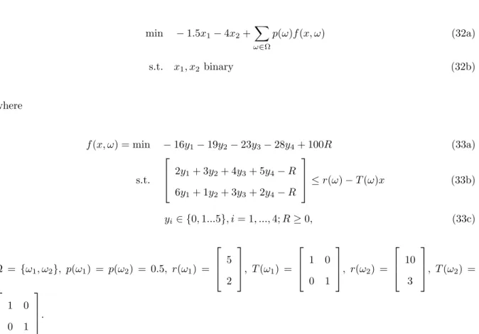
min −1.5x1−4x2+ X ω∈Ω p(ω)f(x, ω) (32a) s.t. x1, x2 binary (32b) where f(x, ω) = min −16y1−19y2−23y3−28y4+ 100R (33a) s.t. 2y1+ 3y2+ 4y3+ 5y4−R 6y1+ 1y2+ 3y3+ 2y4−R ≤r(ω)−T(ω)x (33b) yi∈ {0,1...5}, i= 1, ...,4;R≥0, (33c) Ω = {ω1, ω2}, p(ω1) = p(ω2) = 0.5, r(ω1) = 5 2 , T(ω1) = 1 0 0 1 , r(ω2) = 10 3 , T(ω2) = 1 0 0 1 .
The summary of applying ABCalgorithm withCPT-DandBB-DonExample 1.1are shown in Table 1 and Table 2.
Iter v V x Num Nodes f(x, ω1) Num Cuts f(x, ω2) Num Cuts Value function cut for Node
1 -M-5.5 Inf (1,1) 1 -57 0 -76 1 η≥ −73.7560 + 6.2292x1+ 1.0268x2
2 -76.7292 -72 (0,1) 1 -57 0 -80.625 4 η≥ −80.0714 + 0.8929x1+ 11.2589x2
3 -73.7560 -72.8125 (0,0) 2 -60.2979 6 -80 5 η≥ −70.1489 + 2.4734x1+ 0.9468x2
4 -72.8125 -72 (0,1) 3 -57 0 -80 2 η≥ −79 + 1.4583x1+ 10.5x2
5 -72.5 -72.5 (0,1) 3
Table 1: ABCAlgorithm withCPT-Dfor Example 1.1
Iter v V x Num Nodes f(x, ω1) Num Cuts f(x, ω2) Num Cuts Value function cut for Node
1 -M-5.5 Inf (1,1) 1 -57 0 -76 1 η≥ −73.7560 + 6.2292x1+ 1.0268x2
2 -76.7292 -72 (0,1) 1 -57 0 -80.1250 6 η≥ −79.7232 + 1.5089x1+ 11.1607x2
3 -73.7560 -72 (0,0) 2 -57 6 -80 4 η≥ −68.5 + 2x1
4 -72.5625 -72 (0,1) 2 -57 0 -80 2 η≥ −78.8571 + 1.4643x1+ 10.3571x2
5 -72.5 -72.5 (0,1) 3
Table 2: ABCAlgorithm withBB-D for Example 1.1
In Table 1 and Table 2, the rows show the information generated in each successive iteration of the algorithm. The column header “Num Nodes” indicates the number of active nodes in the B&B tree and
“Num Cuts” indicates the number of multi-term disjunctive cuts generated for that scenario. From the table, we can observe that both algorithms generate more cuts in the subproblem than inExample 1.0
but differences between the execution of BB-DandCPT-Dfor this example are minimal.
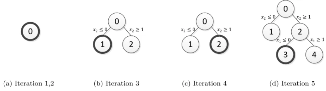
To better illustrate the algorithm, we also include two sets of figures (Figure 1 and Figure 2) which show the master problem B&B tree at each iteration of the algorithm. The node with bold circle contains the solution xk and gets value function updated in the iteration. Similar to the results shown in the tables, there are only minor differences for the master problem B&B tree between the two algorithms.
0 (a) Iteration 1,2 0 1 2 𝑥2≤ 0 𝑥2≥ 1 (b) Iteration 3 0 1 2 3 4 𝑥2≥ 1 𝑥2≤ 0 𝑥1≥ 1 𝑥1≤ 0 (c) Iteration 4 0 1 2 3 4 𝑥2≥ 1 𝑥2≤ 0 𝑥1≥ 1 𝑥1≤ 0 (d) Iteration 5 Figure 1: Master Problem B&B Tree forABCAlgorithm withCPT-Don Example 1.1
0 (a) Iteration 1,2 0 1 2 𝑥2≤ 0 𝑥2≥ 1 (b) Iteration 3 0 1 2 𝑥2≤ 0 𝑥2≥ 1 (c) Iteration 4 0 1 2 3 4 𝑥2≥ 1 𝑥2≤ 0 𝑥1≥ 1 𝑥1≤ 0 (d) Iteration 5 Figure 2: Master Problem B&B Tree forABCAlgorithm withBB-Don Example 1.1
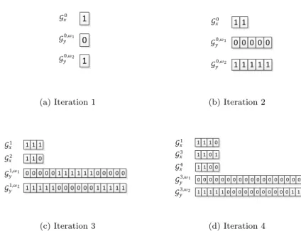
In connection with this illustration, we also present two figures (Figure 3 and Figure 4) which show the encoded sequence for each master problem B&B tree node. With all generated Benders’ cuts as one pool and all generated subproblem’ cuts as another pool, the sequence encodes the validity of the cuts from each pool for any given node of the master problem B&B tree. Again, there are only minor differences in the execution of the two algorithms for this example.
Example 1.2This example extendsExample 1.1by requiring general integer variables in the first
stage as well. So instead of havingx1, x2to be binary, they are now allowed to be integers and bounded
by 0 ≤ x1, x2 ≤ 5. The summaries of applying two algorithms are shown in Table 3 and Table 4.
Compared to the previous example, Tables -(3) and (4) demonstrate that due to a larger number of choices resulting from general integer variables in the first stage, the algorithms require more iterations
𝒢𝑦0,𝜔1 𝒢𝑦0,𝜔2 𝒢𝑥0 0 1 1 (a) Iteration 1 𝒢𝑦0,𝜔1 𝒢𝑦0,𝜔2 𝒢𝑥0 0 0 0 0 1 1 1 1 1 1 1 0 (b) Iteration 2 𝒢𝑦1,𝜔1 𝒢𝑦1,𝜔2 𝒢𝑥1 0 0 0 0 0 1 1 1 1 1 1 1 1 1 1 1 0 0 0 0 0 0 1 1 1 1 1 1 1 1 𝒢𝑥2 1 1 0 0 0 0 0 0 (c) Iteration 3 𝒢𝑦3,𝜔1 𝒢𝑦3,𝜔2 𝒢𝑥1 0 0 0 0 0 0 0 0 0 0 0 1 1 1 1 1 0 0 0 0 0 0 0 0 0 0 1 1 1 𝒢𝑥3 1 1 0 0 0 0 0 0 1 0 0 1 0 0 1 𝒢𝑥4 1 1 0 0 (d) Iteration 4
Figure 3: Gx,Gy forABCAlgorithm withCPT-Don Example 1.1
𝒢𝑦0,𝜔1 𝒢𝑦0,𝜔2 𝒢𝑥0 0 1 1 (a) Iteration 1 𝒢𝑦0,𝜔1 𝒢𝑦0,𝜔2 𝒢𝑥0 0 0 0 0 1 1 1 1 1 1 1 0 0 0 1 1 (b) Iteration 2 𝒢𝑦1,𝜔1 𝒢𝑦1,𝜔2 𝒢𝑥1 0 0 0 0 0 0 0 1 1 1 1 1 1 1 1 1 1 1 0 0 0 0 0 0 1 1 1 1 1 1 𝒢𝑥2 1 1 0 1 1 0 0 0 0 1 (c) Iteration 3 𝒢𝑦2,𝜔1 𝒢𝑦2,𝜔2 𝒢𝑥1 0 0 0 0 0 0 0 0 0 0 0 1 1 1 1 1 1 1 0 0 0 0 0 0 0 0 0 1 1 1 𝒢𝑥2 1 1 0 0 0 0 0 0 1 0 0 1 0 0 0 1 (d) Iteration 4
Figure 4: Gx,Gy forABCAlgorithm withBB-Don Example 1.1
Iter v V x Num Nodes f(x, ω1) Num Cuts f(x, ω2) Num Cuts Value function cut for Node
1 -M-27.5 Inf (5,5) 1 100 0 -47 2 η≥ −261 + 5x1+ 52.5x2
2 -261 -1 (0,0) 1 -60.9545 4 -81.9048 4 η≥ −71.4297 + 3.7564x1+ 1.0352x2
3 -80.3241 -1 (0,3) 2 -19 0 -77.9165 6 η≥ −83.2386 + 11.5934x2
4 -74.3945 -1 (0,1) 3 -57 0 -80 4 η≥ −72.0974 + 1.1915x1+ 3.5974x2
5 -72.5 -72.5 (0,1) 4
Iter v V x Num Nodes f(x, ω1) Num Cuts f(x, ω2) Num Cuts Value function cut for Node 1 -M-27.5 Inf (5,5) 1 100 0 -47 2 η≥ −261 + 5x1+ 52.5x2 2 -261 -1 (0,0) 1 -59.6667 5 -80 5 η≥ −69.8333 + 2x1+ 1.3333x2 3 -77.8333 -1 (0,3) 2 -19 0 -76 3 η≥ −90.25 + 14.25x2 4 -73.6667 -59.5 (3,2) 5 -38 0 -61 5 η≥ −74.1 + 1.8667x1+ 9.5x2 5 -72.75 -62 (2,2) 5 -38 0 -66 6 η≥ −81 + 5x1+ 9.5x2 6 -72.5 -63 (0,1) 5 -57 0 -80 0 η≥ −70.5 + 2x1+ 2x2 7 -72.5 -72.5 (0,1) 5
Table 4: ABCAlgorithm withBB-D for Example 1.2
to solve the problem. Note also that usingBB-Drequires more iterations thanCPT-Dfor this instance, although the average number of cuts forBB-Dis fewer than that used byCPT-D.
Example 1.3 The instance we study below includes mixed-integer variables in both stages, and we
also allow randomness in theT matrix, stated as follows. T(ω1) = 0.1 0 0 0.5 ,T(ω2) = 0.3 0.2 0 0.2 .
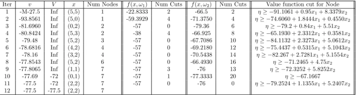
The summary of applying the algorithms are shown in Table 5 and Table 6. From Table (5) and (6)
Iter v V x Num Nodes f(x, ω1) Num Cuts f(x, ω2) Num Cuts Value function cut for Node
1 -M-27.5 Inf (5,5) 1 -22.8333 2 -66.5 2 η≥ −91.1061 + 0.95x1+ 8.3379x2 2 -93.8561 Inf (5,0) 1 -59.3929 4 -71.3750 4 η≥ −74.6060 + 1.8444x1+ 0.4550x2 3 -81.6960 Inf (0,2) 2 -57 0 -79.36 6 η≥ −79.2 + 0.84x1+ 5.51x2 4 -80.8424 Inf (5,3) 2 -38 4 -66.925 8 η≥ −65.1930 + 2.3312x1+ 0.3581x2 5 -79.48 Inf (5,2) 3 -57 0 -67.7086 10 η≥ −84.1132 + 2.3273x1+ 5.0612x2 6 -78.6816 Inf (4,2) 4 -57 0 -69.2180 12 η≥ −75.4437 + 0.5315x1+ 5.1043x2 7 -78.16 Inf (3,2) 4 -57 0 -70.5438 14 η≥ −82.267 + 2.7281x1+ 5.1554x2 8 -77.8543 Inf (5,2) 6 -57 0 -66.4930 16 η≥ −71.2465 + 4.75x2 9 -77.8065 Inf (1,1) 7 -57 3 -76 13 η≥ −72.3252 + 5.8252x2 10 -77.69 -72 (0,1) 7 -57 1 -77.3333 20 η≥ −67.1667 11 -77.5 -72 (2,2) 7 -57 0 -76 0 η≥ −79.2524 + 1.1355x1+ 5.2407x2 12 -77.5 -77.5 (2,2) 7
Table 5: ABCAlgorithm withCPT-Dfor Example 1.3
Iter v V x Num Nodes f(x, ω1) Num Cuts f(x, ω2) Num Cuts Value function cut for Node
1 -M-27.5 Inf (5,5) 1 -22.8333 2 -65.6250 3 η≥ −91.2652 + 1.0375x1+ 8.3697x2 2 -93.5777 Inf (5,0) 1 -57 4 -70.5 4 η≥ −73.6806 + 1.9861x1 3 -81.6806 Inf (0,2) 2 -57 0 -76 4 η≥ −77.2950 + 5.3975x2 4 -80.4686 -74.5 (5,3) 2 -38 6 -64.6375 5 η≥ −65.8580 + 2.7049x1+ 0.3382x2 5 -79.7361 -74.5 (4,2) 3 -57 0 -67.5333 7 η≥ −73.1165 + 0.2569x1+ 4.9111x2 6 -79 -74.5 (3,2) 4 -57 0 -68.4810 10 η≥ −81.0190 + 3.7595x1+ 3.5x2 7 -77.5098 -74.5 (5,2) 5 -57 0 -66 4 η≥ −69.8442 + 1.0174x1+ 1.6287x2 8 -77.5 -77 (2,2) 5 -57 0 -76 0 η≥ −76.0454 + 1.1008x1+ 3.6719x2 9 -77.5 -77.5 (2,2) 5
Table 6: ABCAlgorithm withBB-D for Example 1.3
we can conclude thatBB-Drequires far fewer disjunctive cuts on average for solving subproblems than
CPT-D. In addition, the total number of iterations and Benders’ cuts in the first stage are also fewer.
4.2
Experiments with a Computational Prototype.
In this subsection we report experiments with a Matlab prototype to give the reader a sense of the potential for the methodology presented in this paper. We designed a Matlab implementation of theABC
(e.g. managing the B&B tree) the Matlab script operates in the Matlab environment. Because Matlab is a scripting language, there are large overheads in execution, and in general, cannot be expected to compete with codes written in C or C++. Such handicaps notwithstanding, we conducted an experiment to see how our procedures scale with increases in the number of scenarios. Moreover, we wish to study how a commercial software like CPLEX might perform on the same instances.
Three sets of instances are generated based on Example 1.1-1.3. For each example, we create 4,9,36,121,441,1681,l0201 scenarios by generating the right hand sidesr(ω) from equidistant lattice points in [5,15]×[5,15] with equal probability assigned to each point. This methodology was borrowed from [Ahmed et al., 2004]. For the seven instances based on Example 1.3, we use the same random right hand side r(ω) = r1(ω) r2(ω)
as in Example 1.2, but in addition T(ω) is also random. The entries for these matrices were 0 or 1 with equal probability.
Table 7 compares the performance of three algorithms: two based on using the ABC algorithm
withCPT-Dand BB-Dwhereas, the third algorithm used CPLEX 12.3 (with default setting) for the
MILP formulation of the deterministic equivalent formulation (DEF). All approaches were run on a Windows PC operating with Intel i7-3770K 3.5GHz processors. Instances 1-3 in the table correspond to the variations based on Example 1.1-1.3. The column heading Obj denotes the optimal objective value of the SMIP,Var andConstr denote the number of variables and constraints in theDEF. The entries in column ABC(CPT-D) and ABC(BB-D) denote Iterations (Master Nodes, Second stage Leaf Nodes, Running Time) which correspond to the total number of iterations, the total number of nodes in the B&B tree in the master problem, the maximum leaf nodes encountered during solving the subproblem and the total running time. TheDEF column shows the cpu time required to solveDEF
using the default version CPLEX 12.3 MIP solver. The maximum cpu time allowed was 60 minutes. The results reported in Table 7 clearly demonstrate that the approach of solving a DEP with a commercial solver does not scale well, failing to solve 9 instances for which the number of scenarios were somewhat large. In comparing the performance of ABC(CPT-D)andABC(BB-D), we observe that the former also runs into numerical difficulties for 4 of the larger instances. In contrast, ABC(BB-D)
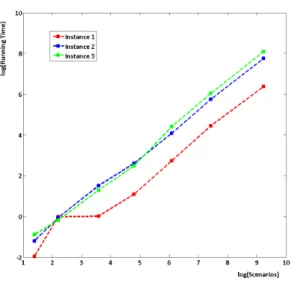
produces optimal solutions for all the instances within very reasonable computational times. From the log-log plot in Figure 5, as number of scenarios increases, the running time also increases polynomially
forABC(BB-D). The slopes of each of the three graphs are slightly larger than one (with values 1.0048,
1.1245, 1.1677) which suggests that as the number of scenarios increases, the running time increases at a rate that is only slightly worse than “linear”. To sum up, based on the instances tested, algorithm
ABCshows very stable results and scales quite well with the number of scenarios. ∗Obj=65.576 and the solution has numerical issues
Scenarios Obj Var Constr ABC(CPT-D) ABC(BB-D) DEF Instance 1 4 -63.50 26 17 7 (4, 5, 0.234) 5 (4,5,0.14) 0.23 9 -66.56 56 37 6 (2, 6, 0.29) 18 (15, 10, 0.98) 0.02 36 -66.83 218 145 7 (2, 7, 1.36) 6 (2, 7, 1.01) 0.02 121 -67.17 728 485 7 (1, 8, 4.43) 6 (1, 8, 2.96) 0.16 441 -65.58 2648 1765 16 (3, 15, 46.63) 10 (2, 7, 15.27) 1.58∗ 1681 -64.72 10088 6725 16 (3, 17, 262.44) 12 (3, 23, 85.29) Failed(>60mins) 10201 -64.19 61208 40805 Numerical Issue 13 (3, 23, 583.08) Failed(>60mins)
Instance 2 4 -63.50 26 17 12 (10, 10, 0.37) 12 (14, 10, 0.3) 0.02 9 -66.56 56 37 20 (15, 10, 1.92) 18 (15, 10, 0.94) 0.02 36 -69.86 218 145 19 (16, 12, 7.64) 18 (16, 10, 4.54) 0.03 121 -71.12 728 485 18 (16, 11, 25.18) 17 (16, 11, 13.51) 4.09 441 -69.64 2648 1765 20 (16, 22, 168.43) 18 (15, 21, 58.97) Failed(>60mins) 1681 -68.85 10088 6725 Numerical Issue 20 (16, 27, 312.36) Failed(>60mins) 10201 -68.45 61208 40805 Numerical Issue 21 (18, 31, 2333.307) Failed(>60mins)
Instance 3 4 -63.50 26 17 10 (6, 7, 0.55) 19 (18,8,0.41) 0.00 9 -64.22 56 37 19 (15, 10, 2.09) 19 (15, 10, 0.83) 0.13 36 -66.42 218 145 25 (21, 12, 7.85) 25 (19, 13, 3.62) 4.18 121 -64.78 728 485 25 (20, 12, 26.94) 25 (19, 13, 12.04) Failed(>60mins) 441 -63.33 2648 1765 28 (21, 24, 222.82) 27 (20, 24, 82.60) Failed(>60mins) 1681 -62.19 10088 6725 31 (22, 28, 1210.94) 28 (23, 33, 419.42) Failed(>60mins) 10201 -61.83 61208 40805 Numerical Issue 31 (24, 34, 3243.82) Failed(>60mins)
Table 7: Comparison of ABCwith DEF
5
Conclusion
As stated at the outset, our paper returns to the general class of two stage SMIP problems that was the focus of the paper by [Carøe and Tind, 1998]. This class of problems involves mixed-integer variables in both stages, and randomness is also allowed in all data elements of the second stage MIP. Despite the elegance of the work of [Carøe and Tind, 1998], the chasm between first and second stage strategies has persisted over the past 15 years. Using several building blocks that have been effective in the interim, we have developed a time-staged decomposition algorithm for very general SMIP models. Other effective ideas, such as allowing the second stage problem to be solved inexactly are also permitted within the overall strategy. The key feature of this algorithm is a first stage B&B process (i.e. the ABC algorithm) which simultaneously guides both the construction of approximations as well as the search for optimal first stage decisions. Furthermore, the value function approximations remain piecewise linear and convex for each first stage B&B node, and similarly, the second stage relaxations (built using multi-term disjunctions) are also polyhedral. While these elements maintain convex building blocks, the overall search is facilitated by an encoding strategy (to record approximations) that allows us to approximate severe non-convexities typical of general SMIP models. This encoding mechanism is analogous to the way in which chromosomes are passed from generation to generation in nature.
We have presented a preliminary computational study in which a commercial LP solver was guided by a Matlab-based script, and this implementation was compared with a state-of-the-art MIP solver to obtain a solution for a deterministic extensive form SMIP. Our computations reveal that as the number of scenarios grow, our Matlab-guided implementation was faster and more stable than the commercial solver for an extensive form SMIP. We expect that future implementations using C/C++ programming will yield far greater capabilities.
Appendix: Example 1.0
Consider the following example that is shown in [Sen et al., 2003] which is a variation of an example from ([Schultz et al., 1998]).
min −1.5x1−4x2+ X
ω∈Ω
p(ω)f(x, ω) (34a)
where f(x, ω) = min −16y1−19y2−23y3−28y4+ 100R (35a) s.t. 2y1+ 3y2+ 4y3+ 5y4−R 6y1+ 1y2+ 3y3+ 2y4−R ≤r(ω)−T(ω)x (35b) yi binaryi= 1, ...,4, R≥0, (35c) Ω = {ω1, ω2}, p(ω1) = p(ω2) = 0.5, r(ω1) = 5 2 , T(ω1) = 1 0 0 1 , r(ω2) = 10 3 , T(ω2) = 1 0 0 1
. We first apply theABCalgorithm withCPT-Dto solve this example.
At iterationk= 1, the algorithm starts from solving the LP relaxed master problem withη bounded.
min −1.5x1−4x2+η (36a)
s.t. x1, x2 binary (36b)
η ≥ −M (36c)
We get solution (x1, x2, η) = (1,1,−M) with objectivev=−M−5.5. Here only the root node is in the B&B tree. x= (1,1) withQo
1={0≤x1≤1,0≤x2≤1}is inserted into subproblems. Then CPT-D
is called for eachω∈Ω.
For ω1, fL(x, ω1) is solved and we get y(ω1) = (0,1,0,0.5,0). y4 is fractional and partitions are
formed for integer variables: {y4≤0} ∩Q2 or{y4≥1} ∩Q2. The cut derived from CGLP forx∈Qo1 is
−2y2−2y4+ 2R≥ −4 + 2x2. (37)
After adding the cut, fL(x, ω1) is re-optimized and the solution is y(ω1) = (0,0,0,1,0). It satisfies
integer constraints. So no more cuts are generated in this iteration.
For ω2, fL(x, ω2) is solved and we get y(ω2) = (0,1,0,0,0). Again, this solution satisfies integer
constraints, and hence, no cuts are needed. All scenarios have integer solution, soV is updated. V =−29. The value function cut for x∈Qo
1 is
At iteration k = 2, the master problem continues to be solved by B&B method. We get solution (x1, x2, η) = (1,0,−40) with objectivev=−41.5. Still only the root node is in the B&B tree. x= (1,0)
withQo
1={0≤x1≤1,0≤x2≤1}is inserted into subproblems. CPT-Dis called for eachω∈Ω.
Forω1,fL(x, ω) is initialized as follows:
fL(x, ω1) = min −16y1−19y2−23y3−28y4+ 100R (39a)
s.t. 2y1+ 3y2+ 4y3+ 5y4−R≤5−x1 (39b)
6y1+ 1y2+ 3y3+ 2y4−R≤2−x2 (39c)
−2y2−2y4+ 2R≥ −4 + 2x2 (39d)
0≤yi≤1i= 1, ...,4, R≥0 (39e)
where constraint (39d) is from cut (37) generated in iteration 1. (39) is solved and we get y(ω1) =
(0,1,0,1,0). It satisfies integer constraints. So no cuts are needed.
For ω2, fL(x, ω2) is solved and we get y(ω2) = (0.1154,1,0,0.1538,0). y1 is the variable we choose
to split. The partitions we form are: {y1 ≤0} ∩Q2 or {y1≥1} ∩Q2. The cut derived from CGLP for x∈Qo
1is
−4.875y2−6.5y4+ 1.625R≥ −6.5 + 1.625x1. (40)
After adding the cut,fL(x, ω2) is re-optimized and the solution is
y(ω2) = (0.056,1,0.222,0,0). (41)
Since y(ω2) is located on the root node, no more splits are needed. The same partition is used: {y1≤
0} ∩Q2 or{y1≥1} ∩Q2. The cut derived from CGLP forx∈Qo1 is
−2.25y2−4.5y3+ 2.25R≥ −2.25. (42)
After adding the cut,fL(x, ω2) is re-optimized and the new solution isy(ω2) = (0.06,0.68,0.16,0.24,0).
Again,y(ω2) is located on the root node, and no more splits are needed. The same partition: {y1≤0}∩Q2
or{y1≥1} ∩Q2 is used to formulate CGLP. With onlyy(ω2) changed, another cut derived from CGLP
forx∈Qo
1 is
−2.5y3−2.5y4+ 2.5R≥ −2.5 + 2.5x1. (43)
After adding the cut, fL(x, ω2) is re-optimized and the solution is y(ω2) = (0.1667,1,0,0,0). y(ω2)
{y1≥1} ∩Q2is used to formulate CGLP. The cut derived from CGLP forx∈Qo1is
−6y1+ 1.5R≥0. (44)
After adding the cut, fL(x, ω2) is re-optimized and the solution is y(ω2) = (0,1,0,0,0). It satisfies
integer constraints. So no more cuts are needed. All scenarios have integer solution, so V is updated. V =−34.5
The value function cut for x∈Qo
1 is
−7.55x1−3.8333x2+η≥ −40.55. (45)
At iterationk= 3, the master problem continues to be solved by the B&B method. We get solution (x1, x2, η) = (0,0,−40) with objectivev=−40. The solution is on node 1 withQ11={0≤x1≤0,0≤ x2≤1}. Hencex= (0,0) andQ11 are treated as input parameters forCPT-Dfor eachω∈Ω.
Forω1, 0 cuts are needed. The solution isy(ω1) = (0,1,0,1,0).
Forω2, 1 cut is needed (shown below). The solution isy(ω1) = (0,0,0,1,0).
−3.6923y2−2.4615y3−3.6923y4+ 1.2308R≥ −3.6923. (46) V is updated. V =−37.5 and the value function cut forQ11 is
−8.3333x2+η≥ −37.5 (47)
At iteration k= 4, with updated value function cut for node 1, the master problem continues to be solve by B&B method. We get solution (x1, x2, η) = (0,0,−37.5) with objective v=−37.5. V −v ≤.
The algorithm stops
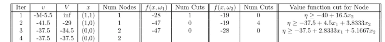
A short summary of using ABCalgorithm withCPT-Dto solve this problem is shown in Table 8.
Iter v V x Num Nodes f(x, ω1) Num Cuts f(x, ω2) Num Cuts Value function cut for Node
1 -M-5.5 inf (1,1) 1 -28 1 -19 0 η≥ −40 + 16.5x2
2 -41.5 -29 (1,0) 1 -47 0 -19 4 η≥ −40.55 + 7.55x1+ 3.8333x2
3 -40 -34.5 (0,0) 2 -47 0 -28 1 η≥ −37.5 + 8.3333x2
4 -37.5 -37.5 (0,0) 2
Table 8: ABCAlgorithm withCPT-Dfor Example 1.0
Each row shows the information for one iteration. Column “Num Nodes” denotes the number of active nodes in the B&B tree. “Num Cuts” means the number of multi-term disjunctive cuts generated for that scenario.
from solving the LP relaxed master problem withη bounded.
At iteration k= 1, We get solution (x1, x2, η) = (1,1,−M) with objectivev =−M −5.5 from the
B&B method. x= (1,1) with Qo
1={0≤x1≤1,0≤x2≤1} is inserted intoBB-Dfor eachω∈Ω.
For ω1, f(x, ω1) is solved by the B&B method and we get 2 nodes inT2. With 1 cut derived from
CGLP forx∈Qo
1:
−2y2−2y4+ 2R≥ −4 + 2x2, (48)
the solution falls intoT2 and no more cuts are needed. y(ω1) = (0,0,0,1,0).
For ω2,f(x, ω2) is solved by B&B method and we get 1 nodes in T2. No cuts are needed. y(ω2) =
(0,1,0,0,0). All scenarios have integer solution, soV is updated. V =−29 The value function cut for x∈Qo1 is
−16.5x2+η≥ −40 (49)
At iteration k = 2, the master problem continues to be solved by B&B method. We get solution (x1, x2, η) = (1,0,−40) with objective v = −41.5. x = (1,0) with Qo1 ={0 ≤x1 ≤1,0 ≤x2 ≤1} is
inserted into subproblems. CPT-Dis called for eachω∈Ω. Forω1,f(x, ω1) is initialized as follows:
f(x, ω1) = min −16y1−19y2−23y3−28y4+ 100R (50a)
s.t. 2y1+ 3y2+ 4y3+ 5y4−R≤5−x1 (50b)
6y1+ 1y2+ 3y3+ 2y4−R≤2−x2 (50c)
−2y2−2y4+ 2R≥ −4 + 2x2 (50d)
yi binaryi= 1, ...,4, R≥0 (50e)
where constraint (50d) is from cut (48) generated in iteration 1. (50) is solved by B&B method and we getT2 with 1 node. So no cuts are needed. y(ω1) = (0,1,0,1,0).
Forω2,f(x, ω2) is solved by B&B method and we getT2with 4 nodes. 4 cuts are derived from CGLP
forx∈Qo1: −8.6667y1+ 2.1667R≥0 −4y3+ 4R≥0 −3.75y2−5y4+ 1.25R≥ −5 −x1−y4+R≥ −1 (51)
With 4 cuts added, the solutiony(ω1) = (0,1,0,1,0).
All scenarios have integer solution, soV is updated. V =−34.5 The value function cut for x∈Qo
1 is
−4.5x1−3.8333x2+η≥ −37.5. (52)
At iteration k = 3, the master problem continues to be solve by B&B method. We get solution (x1, x2, η) = (0,0,−37.5) with objective v = −37.5. The solution is on node 2 with Q11 ={0 ≤x1 ≤
1,0≤x2≤0}. x= (0,0) andQ21 are treated as input parameters forBB-Dfor eachω∈Ω.
Forω1, 0 cuts are needed. The solution isy(ω1) = (0,1,0,1,0).
For ω2, 0 cuts are needed. The solution isy(ω1) = (0,0,0,1,0). V is updated. V =−37.5 and the
value function cut forQ2 1is
−2.8333x1−5.1667x2+η≥ −37.5 (53)
At iteration k= 4, with updated value function cut for node 2, the master problem continues to be solve by B&B method. We get solution (x1, x2, η) = (0,0,−37.5) with objective v=−37.5. V −v ≤.
The algorithm stops
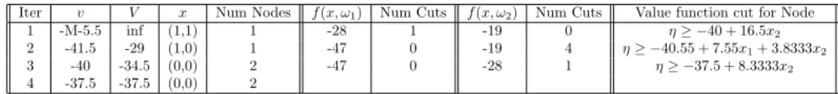
A short summary of usingABCalgorithm withBB-Dto solve this problem is shown in Table 9. As
Iter v V x Num Nodes f(x, ω1) Num Cuts f(x, ω2) Num Cuts Value function cut for Node
1 -M-5.5 inf (1,1) 1 -28 1 -19 0 η≥ −40 + 16.5x2
2 -41.5 -29 (1,0) 1 -47 0 -19 4 η≥ −37.5 + 4.5x1+ 3.8333x2
3 -37.5 -34.5 (0,0) 2 -47 0 -28 0 η≥ −37.5 + 2.8333x1+ 5.1667x2
4 -37.5 -37.5 (0,0) 2
Table 9: ABCAlgorithm withBB-D for Example 1.0
you may notice, there is only small difference betweenBB-DandCPT-DforExample 1. At iteration 2, becauseBB-Duses partitions with 4 terms to generate cuts from the beginning, the quality of the cut is better thanCPT-Dwhich results in no more cuts needed for subproblems in the following iterations. But CGLP with 4 terms take more time to solve.
References
[Ahmed et al., 2004] Ahmed, S., Tawarmalani, M., and Sahinidis, N. V. (2004). A finite branch-and-bound algorithm for two-stage stochastic integer programs. Mathematical Programming, 100(2):355– 377.
[Balas et al., 1993] Balas, E., Ceria, S., and Cornu´ejols, G. (1993). A lift-and-project cutting plane algorithm for mixed 0-1 programs. Mathematical Programming, 58:295–324.
[Carøe and Tind, 1998] Carøe, C. and Tind, J. (1998). L-shaped decomposition of two-stage stochastic programs with integer recourse. Mathematical Programming, 83:451–464.
[Carøe and Schultz, 1997] Carøe, C. C. and Schultz, R. (1997). Dual decomposition in stochastic integer programming. Operations Research Letters, 24:37–45.
[Carøe and Schultz, 1998] Carøe, C. C. and Schultz, R. (1998). A two-stage stochastic program for unit commitment under uncertainty in a hydro-thermal power system. InPreprint SC 98-11, Konrad-Zuse-Zentrum fur Informationstechnik, pages 98–13.
[Chen et al., 2011] Chen, B., K¨u¸c¨ukyavuz, S., and Sen, S. (2011). Finite disjunctive programming char-acterizations for general mixed integer linear programs. Operations Research, 59(1):202–210.
[Chen et al., 2012] Chen, B., K¨u¸c¨ukyavuz, S., and Sen, S. (2012). A computational study of the cutting plane tree algorithm for general mixed-integer linear programs. Operations Research Letters, 40(1):15 – 19.
[Escudero et al., 2007] Escudero, L., Garn, A., Merino, M., and P´erez, G. (2007). A two-stage stochastic integer programming approach as a mixture of branch-and-fix coordination and benders decomposition schemes. Annals of Operations Research, 152:395–420. 10.1007/s10479-006-0138-0.
[Gade et al., 2012] Gade, D., K¨u¸c¨ukyavuz, S., and Sen, S. (2012). Decomposition algorithms with para-metric gomory cuts for two-stage stochastic integer programs. Mathematical Programming, pages 1–26.
[Higle and Sen, 1994] Higle, J. L. and Sen, S. (1994). Finite master programs in regularized stochastic decomposition. Mathematical Programming, 67(1-3):143–168.
[Kong et al., 2006] Kong, N., Schaefer, A. J., and Hunsaker, B. (2006). Two-stage integer programs with stochastic right-hand sides. Mathematical Programming, 108(24):275–296.
[Louveaux and Schultz, 2003] Louveaux, F. and Schultz, R. (2003). Stochastic integer programming. Handbooks in Operations Research and Management Science, 10:213–266.
[Lulli and Sen, 2004] Lulli, G. and Sen, S. (2004). A branch-and-price algorithm for multistage stochas-tic integer programming with application to stochasstochas-tic batch-sizing problems. Management Science, 50(6):786–796.