brain-computer interface
.
White Rose Research Online URL for this paper:
http://eprints.whiterose.ac.uk/147288/
Version: Accepted Version
Article:
Azab, A., Mihaylova, L. orcid.org/0000-0001-5856-2223, Ang, K.K. et al. (1 more author)
(2019) Weighted transfer learning for improving motor imagery-based brain-computer
interface. IEEE Transactions on Neural Systems and Rehabilitation Engineering. ISSN
1534-4320
https://doi.org/10.1109/TNSRE.2019.2923315
© 2019 IEEE. Personal use of this material is permitted. Permission from IEEE must be
obtained for all other users, including reprinting/ republishing this material for advertising or
promotional purposes, creating new collective works for resale or redistribution to servers
or lists, or reuse of any copyrighted components of this work in other works. Reproduced
in accordance with the publisher's self-archiving policy.
[email protected] https://eprints.whiterose.ac.uk/
Reuse
Items deposited in White Rose Research Online are protected by copyright, with all rights reserved unless indicated otherwise. They may be downloaded and/or printed for private study, or other acts as permitted by national copyright laws. The publisher or other rights holders may allow further reproduction and re-use of the full text version. This is indicated by the licence information on the White Rose Research Online record for the item.
Takedown
If you consider content in White Rose Research Online to be in breach of UK law, please notify us by
Weighted Transfer Learning for Improving Motor
Imagery-based Brain-computer Interface
Ahmed M. Azab,
Student member, IEEE,
Lyudmila Mihaylova,
Senior Member, IEEE,
Kai Keng Ang,
Senior
Member, IEEE
, and Mahnaz Arvaneh,
Member, IEEE
Abstract—One of the major limitations of motor imagery (MI)-based brain-computer interface (BCI) is its long calibration time. Due to between sessions/subjects variations in the properties of brain signals, typically a large amount of training data needs to be collected at the beginning of each session to calibrate the parameters of the BCI system for the target user. In this paper, we propose a novel transfer learning approach on the classification domain to reduce the calibration time without sacrificing the classification accuracy of MI-BCI. Thus, when only few subject-specific trials are available for training, the estimation of the classification parameters is improved by incorporating previously recorded data from other users. For this purpose, a regularization parameter is added to the objective function of the classifier to make the classification parameters as close as possible to the classification parameters of the previous users who have feature spaces similar to that of the target subject. In this study, a new similarity measure based on the kullback leibler divergence (KL) is used to measure similarity between two feature spaces obtained using subject-specific common spa-tial patterns (CSP). The proposed transfer learning approach is applied on the logistic regression classifier and evaluated using three datasets. The results showed that compared to the subject-specific classifier, the proposed weighted transfer learning classifier improved the classification results particularly when few subject-specific trials were available for training (p <0.05). Importantly, this improvement was more pronounced for users with medium and poor accuracy. Moreover, the statistical results showed that the proposed weighted transfer learning classifier performed significantly better than the considered comparable baseline algorithms.
Index Terms—Brain computer interface, Transfer learning, Logistic regression, Motor imagery.
I. INTRODUCTION
B
RAIN-computer interface (BCI) provides a direct com-munication between a person’s brain and an electronic device without the need for any muscle control [1], [2]. Electroencephalogram (EEG) is the most widely used brain signals in BCI since it is measured non-invasively with a high temporal resolution [2], [3]. Different neurophysiological pat-terns of EEG have been used to operate BCIs, such as steady state visual evoked potentials, P300, readiness potentials and motor imagery [4]. Among them motor imagery (MI) has attracted increased attention, as unlike many other types ofAhmed M. Azab, Lyudmila Mihaylova, and Mahnaz Arvaneh are with the Department of Automatic Control and System Engineering, Sheffield University, United Kingdom. e-mail:[email protected], [email protected], [email protected]
Kai Keng Ang is with Institute for Infocomm Research, Agency for Science, Technology and Research (A*STAR), Singapore and with School of Computer Science and Engineering, Nanyang Technological University, Singapore e-mail: [email protected]
BCI, MI-based BCI does not require any external stimuli and can be used in a self-paced way which is closer to a natural and intuitive control [5].
Despite several recent advances, most of the MI-based BCI applications are still limited to the laboratory due to their long calibration time. As the literature shows [6]–[8], due to considerable inter-subject and inter-session variations, a reliable machine learning model that performs well across all sessions and subjects has not been feasible yet. Consequently, a 20-30 minutes calibration phase at the beginning of each new session is typically conducted to acquire sufficient labeled data to train the subject-specific BCI model. This calibration phase is time consuming and fatiguing, leaving a reduced amount of time for real BCI interactions [9]. Thus, developing reliable methods and approaches that reduce calibration time while keeping accuracy in an acceptable range is highly desirable in MI-based BCI research [7], [9], [10].
One potential approach to reduce the calibration time is transfer learning, where data from other sessions or subjects are mined and used to compensate the lack of labeled data from the current target user [11]. Transfer learning aims at learning characteristics that are consistent across sessions and subjects and at the same time adjusting those characteristics to the available target subject’s few trials. Indeed, how to do transfer learning is not a trivial task, due to the non-stationarity inherent in EEG signals [11], [12]. Transfer learning has been successfully applied in different machine learning applications such as: text, image, and human activity classification [13].
In MI-based BCIs, transfer learning can be applied on either raw EEG, feature or classification domains. The proposed transfer learning algorithms on raw EEG have been mostly based on either importance sampling cross validation [14], [15] or instance selection [16], [17]. For example, a covariate shift adaptation has been proposed in [14], where data from other subjects were weighted based on importance sampling cross-validation. The parts with high weights were then used to estimate the final prediction function. In [16], [17], an instance selection approach has been proposed based on active learning to select trials that were close to the few informative trials of the new subject. The selected trials were added to the existing labeled trials of the new subject to train the BCI model.
In the feature domain, most of the proposed transfer learning algorithms focus on improving common spatial patterns (CSP) through modification of either the covariance matrix estimation method [18], [19] or the CSP optimization function [20], [21]. As an example, Samek et al. in [19] have proposed an extension of CSP, where stationary information across multiple
subjects instead of discriminative information was transferred by learning a stationary subspace.
Domain adaptation techniques [22]–[24] and ensemble learning of classifiers [10], [25] have been adapted in many existing MI-based BCI transfer learning algorithms on the classification domain. In the domain adaptation, the source domain classifier is used for a target domain while its param-eters are adjusted with respect to the target data. Different from the domain adaptation, ensemble learning of classifiers combines different classifiers trained from different source domains to acquire better classification accuracy on the target domain. Recently an application of multi-task learning has been proposed in BCI [26], [27] where the classification parameters of multiple subjects were learned jointly such that the average total errors as well as dissimilarities between the parameters of the different classifiers were minimized. Despite success to some extent, the proposed algorithm is computationally expensive as a big number of parameters need to be optimized simultaneously. Moreover, it does not consider similarities/dissimilarities between the data from the new subject and the existing data from other subjects during the learning process.
This paper proposes a novel transfer learning approach in the classification domain to improve the MI-based BCI performance when only a few subject-specific trials are avail-able for training. In the proposed approach, the classification parameters of each available subject with relatively large num-ber of trials are calculated independently by minimizing the subject-specific classification error. To cope with the problem of having small train data for a new subject, we hypothesize that there is some common information across the subjects performing the same mental tasks (i.e. MI). Following this assumption, the classification parameters of the new target subject with few labeled trials are calculated such that not only the classification error is minimized but also the classification parameters of this target subject get as close as possible to the classification parameters of other existing subjects. This is achieved by adding a regularization term into the classification objective function making a trade-off between minimizing the classification error of the new subject and dissimilarities with the classification parameters of previous users.
It is important to consider that the above-mentioned transfer learning approach may not be very precise for MI-based BCIs that use CSP features, since using the subject-specific CSP for feature extraction leads to different feature spaces for different subjects. To address this issue, we assume, with a fixed coordinate of electrodes, these feature spaces are still relevant as EEG signals are originated from roughly the same areas of the brain for the same motor imagery task leading to nearly similar CSP weights for corresponding channels. Consequently, to transfer the classification parameters across different CSP feature spaces, we link the features of different subjects with the features of the target subject through a new similarity measure obtained using KL divergence. Therefore, the proposed transfer learning approach is further improved by assigning different weights to the previous subjects based on the similarities between their features and the features of the new subject.
The proposed approach is applied on a logistic regression classifier with and without considering similarity weights. The proposed classifiers are evaluated using three datasets with large, moderate, and small number of subjects. The performance of the proposed classifiers are also compared with the results of two state-of-the-art algorithms.
Our results suggest that the proposed weighted transfer learning approach could significantly reduce the required cali-bration time and also enhance the average classification accu-racy, particularly when there are enough previously recorded EEG sessions available for transfer learning. Moreover, the obtained results showed that the proposed weighted transfer learning algorithms significantly outperformed the baseline algorithms.
II. METHODOLOGY
In this paper, we assume that multiple EEG sessions pre-viously recorded from different subjects or from the same subject are available. Given s∈ {1, ..., m} as one of the previously recorded sessions, the set of labeled EEG trials from session s can be presented as ds= (x
i s, y i s) ns i =1, where xisandysi respectively denote the feature vector and the class
label of theith
trial, andnsrefers to the total number of the
trials. Thus, the feature matrix for the sessionsis presented as Xs= [x1s,x2s, ...,x
ns
s ], where Xs∈R
v×ns andv is the number
of features per trial. Subsequently, the label vector is presented as Ys= [ys1, ys2, ..., y
ns
s ], where y i
s∈ {0,1}.
This paper assumes that previously recorded sessions have sufficiently large numbers of labeled trials, whereas the new target subject has only few labeled trials available. Typically, a predictive function,f(.), is trained using the available subject-specific training features to predict the labels of the unlabeled trials. However, when only few labeled trials are available for training, the estimation of the joint distributionP(Xs,Ys)may
not be sufficiently accurate. Hence, the predictive function trained using few trials is often not optimal. This paper proposes a number of transfer learning algorithms to improve the estimation of the predictive function of the new target subject using previously recorded EEG data. Indeed, how to do transfer learning is not a trivial task, due to the non-stationarity inherent in EEG signalsP(Xs,Ys)6=P(Xt,Yt), wheretrefers
to the new target subject.
A. Proposed Logistic Regression-based Transfer Learning Al-gorithm (LTL)
A logistic regression model provides probabilistic predic-tions by transforming a linear model through a logistic sigmoid function as [28]: P(yi s=1|x i s;ws) = 1 1 +exp−(wTsxis), (1)
where s denotes the session s, and ws∈R
v×1 refers to the
classification parameters being used to predict the class labels of the trials Xs. The obtained probabilistic prediction is then
used to predict the class label.
The proposed LTL algorithm consists of two main steps. In the first step, for every previously recorded session,∀ds∈
{d1, d2, ..., dm}, the classification parameters,ws, are
calcu-lated using the following objective function [29]: L1(ws) = min ws ns X i=1 H(ws;ysi,xis) +λs||ws||2 2 ! , (2) where H and ||.||2 denote the cross-entropy and 2-norm
functions respectively. In fact, in L1(ws), the cross entropy
aims at finding ws that minimizes the error rate while the
2-norm penalizes large values of wsto reduce the risk of
over-fitting. The subject-specific regularization parameterλsis used
to control the degree of penalization. Cross entropy function H is also called negative log-likelihood where its minimization is equivalent to maximizing the log likelihood [28], [30], as follows [31]: H(ws;x i s, y i s) =−y i slogP(y i s=1|x i s;ws)−(1−y i s) log(1−P(yi s=1|x i s;ws)), (3) whereP(yi s=1|x i
s;ws)is calculated using (1). The objective
function L1(ws)does not have a closed form solution.
How-ever, it has a unique minimum that can be found using simple and effective iterative approaches such as the gradient descent or Newton’s methods [28], [32].
Despite being sufficiently effective for sessions with large training data sizes, the objective function L1(ws) may fail
in estimating the classification parameters of the new subject since few available subject-specific trials typically are not able to accurately represent the distributions of the features. Thus, to estimate the classification parameters of the new subject, L1(ws)is modified such that not only the error rate
is minimized, but also the estimated classification parameters get as close as possible to the classification parameters of the other existing sessions. In other words, in addition to the discriminative parameters, we are interested in parameters that are similar to the classification parameters of the other sessions with this assumption that there is some common information across the sessions performing the same mental tasks (i.e. motor imagery).
Given the above-mentioned assumption, after calculating the classification parameters of the previously recorded sessions using (2), in the second step, the classification parameters of the new target subject, wt, is calculated using the following
objective function: L2(wt) = min wt nt X i=1 H(wt;y i t,x i t) +λtRT L(wt) ! , (4) where RT L is the regularization term penalizing
dissimilar-ities between wt and the previously calculated ws, ∀ds ∈
{d1, d2, ..., dm}. The regularization parameter λt is making
a trade-off between minimizing the error and dissimilarities between the new target subject and previous sessions in terms of the classification parameters. The term RT L is calculated
by taking into account the prior distribution of the existing classification parameters and comparing them withwtas [27]:
RT L(wt) = 0.5[(wt−µ)TΣT L−1(wt−µ) + log(|ΣT L|)], (5)
whereµandΣT L are respectively calculated as follows: µ= (1/m) m X s=1 ws, (6) ΣT L= diag(Pm s=1(ws−µ)(ws−µ)T) trace(Pm s=1(ws−µ)(ws−µ)T). (7)
As can be seen in (7), ΣT L ∈ Rv×v only includes the
normalized diagonal elements of the covariance matrix, where diag and trace give the diagonal elements and the sum of the diagonal elements of a matrix respectively. Indeed, in this study, only diagonal elements are used to reduce the optimization complexity. Subsequently, in (5), ΣT L is used
to normalize the divergence of each parameter ofwtfrom the
average of the corresponding parameters of the other classifier.
B. Proposed Weighted Logistic Regression-based Transfer Learning Algorithm
The proposed LTL algorithm attempts to improve the es-timation of the classification parameters of a new subject by incorporating the data from previously recorded sessions. However, it treats different feature spaces from the previous sessions similarly, whereas the distribution of EEG signals can be different from session to session and from subject to subject, leading to different subject-specific CSP feature spaces. Thus, depending on the distributions of EEG signals, the EEG features of the new subject might be similar to the EEG features of some of the previously recorded ses-sions while very different from those of some others. Thus, taking into account these differences might further improve the estimation of the classification parameters for a new subject. To address this issue, in the proposed weighted logistic regression-based transfer learning algorithm different weights are allocated to the previously recorded sessions to represent similarities between these sessions and the new subject in terms of distributions of the features.
Kullback-Leibler (KL) divergence is frequently used in the literature to calculate similarities between two sets of EEG features [33]. Since in MI-based BCIs the features are typically normalized log-power of CSP filtered EEG data, they are commonly assumed normally distributed [21]. Thus, in this paper, the KL divergence between two normal distributions are used to measure divergence between EEG features.
Given two normal distributions presented as N0(µ0,Σ0)
andN1(µ1,Σ1), the KL divergence has the following closed
form [33], KL[N0||N1] = 0.5[(µ1−µ0)TΣ−11(µ1−µ0) +trace(Σ−1 1 Σ0)−ln det(Σ0) det(Σ1) −K], (8)
where det,TandKdenote the determinant function, transpose of the matrix, and the dimension of the data, respectively. In this paper, the total divergence between the features of two EEG sessions, KL, can be calculated in two ways, namely¯ supervised and unsupervised. In the supervised case, the total divergence is calculated by averaging the KL divergences calculated for each class separately. On the other hand, in
the unsupervised case, the total divergence equals to the KL divergence between the two sessions without considering the class labels. Subsequently, the similarity weight αs between
the feature sets of the target subjectdtand the feature sets of
each of the previous sessions/subjects ds, is calculated as:
αs= (1/(KL¯ [dt, ds] +ǫ)4) m P i=1 (1/(KL¯ [dt, di] +ǫ)4) , (9)
whereKL is the total divergence calculated using the features¯ distributions of the few available training trials of the target subjectdt(i.e. 10, 20 or all trials per class depending on how
many trials are defined as available) and the available trials from the previous subject/session ds. In (9), ǫ = 0.0001 is
used to ensure the stability of the equation when KL¯ [dt, ds]
gets equal to zero due to having two compared distributions completely similar. Although, this is a very rare event, we must take into account the possibility of unseen events. The power of 4 is applied to the inverse of KL between the distribution of two feature sets to give larger weights to more similar distri-butions and smaller weights to less similar distridistri-butions. This results in an increased sparsity in the similarity weights αs.
Finally, the similarity weight, proposed in (9), is normalized by dividing it to the sum of all similarity measurements between the feature sets of the new target subject and all other available subjects.
The proposed weighted logistic regression-based transfer learning algorithm has the same steps as the proposed LTL. However, instead of equal weights, different weights are assigned to the previously recorded sessions using (9). Ac-cordingly, the new weighted µis obtained as [34]
µw= m X
s=1
αsws. (10)
Likewise, the weightedΣT Lis calculated as
ΣT Lw=
diag(Pm
s=1(αsws−µw)(αsws−µw)T)
trace(Pm
s=1(αsws−µw)(αsws−µw)T). (11)
Finally, RT L in (5) is calculated by replacing µ and ΣT L
withµw andΣT Lw respectively. Considering the two
above-mentioned ways to calculate the similarity weights, the pro-posed weighted algorithms are referred to as either supervised weighted logistic regression-based transfer learning (S-wLTL) or unsupervised weighted logistic regression-based transfer learning (Us-wLTL) in the remaining parts of this paper.
III. EXPERIMENTS A. Data Description
In order to evaluate the proposed algorithms, a dataset from [35], dataset 2a from BCI Competition IV 2008 [36], [37] and dataset IVa from BCI Competition III [38] were used.
Dataset 1: EEG was collected from 19 healthy subjects using 27 channels. For each subject, EEG data were collected without feedback in two sessions conducted on separate days. In this paper, we used only motor imagery data recorded in the first session. This MI part of the dataset consisted of two
runs of EEG recording where the subjects were instructed to perform MI of the chosen hand versus background rest condition. Each run comprised of 40 trials of MI and 40 trials of background rest condition. Thus, in total, there were 160 trials per subject recorded without feedback.
Dataset 2 (Dataset 2a from BCI Competition IV): This dataset consists of EEG data recorded from 9 subjects using 22 electrodes. During the recording sessions, the subjects were instructed to perform one of the four following motor imagery tasks: left hand, right hand, foot or tongue. Two sessions on different days were recorded for each subject with a total of 288 trials per session. In this paper, only data from right and left-hand motor imagery were used. Moreover, only data recorded from the second day were used due to the practical assumption that the training and the testing data of a new subject are recorded on the same day.
Dataset 3 (Dataset IVa from BCI Competition III): This dataset includes EEG signals from five subjects. EEG was recorded using 118 electrodes. It contains data from two classes of right hand and foot imagery. In total, there are 280 trials per subject all recorded on the same day without receiving feedback.
B. Data Processing
A single elliptic bandpass filter from 8 to 30 Hz was used for filtering the EEG data as recommended in [39]–[41], since this single frequency band includes the range of frequencies that are mainly involved in performing motor imagery. Then, CSP were computed for each previous subject independently. Similarly, for the new subject, the CSP filters were calculated only using the available subject-specific training trials. After that, the spatially filtered signals were obtained using the first and the last three spatial filters of CSP as recommended in [42]. Finally, the normalized log band power of the spatially filtered signals were obtained as the features.
For each subject of the three datasets the first 80 trials were considered as the training set and the remaining trials were used as the testing set. To assess the performance of the proposed transfer learning algorithms, three different numbers of training trials were examined for the new subjects; i.e. the first 10 and 20 training trials per class as well as all the training trials were used in order to form the subject-specific training set. Besides, all the available training trials of the other subjects from the same dataset were used for transfer learning. The regularization parameters, λs andλt, were selected from
21 values which satisfy ei
, where i ∈ {−1,−0.9, ...,0.9,1}. 5-fold cross-validation was performed for each subject using the available training trials to select the best regularization parameters.
The results of the proposed transfer learning algorithms were compared with two baseline algorithms. The first algo-rithm is the commonly used subject-specific (SS) BCI model where the support vector machine (SVM) classifier is trained independent from other subjects using features extracted from CSP algorithm similar to what suggested in [6], [39], [43]. This algorithm is abbreviated as (SS) in the rest of the paper. logistic regression classifier was not included as a classifier
TABLE I
CLASSIFICATION ACCURACIES CALCULATED USING THE BASELINE ALGORITHMS(SS,ANDMT-L)AND THE PROPOSED ALGORITHMS(LTL, S-WLTL,
ANDUS-WLTL)WHEN ONLY10TRIALS PER CLASS WERE AVAILABLE FOR TRAINING FROM THE NEW SUBJECT. THE RESULTS OF ALL DATASETS SHOW
THAT THE PROPOSED WEIGHTED LOGISTIC TRANSFER LEARNING ALGORITHMS(S-WLTLANDUS-WLTL)OUTPERFORMED THE REST.
Dataset 1 Overall
Algorithm sub1 sub2 sub3 sub4 sub5 sub6 sub7 sub8 sub9 sub10 sub11 sub12 sub13 sub14 sub15 sub16 sub17 sub18 sub19 Mean Std
SS 64 55 55 60 69 72 47 90 81 52 48 84 54 76 50 64 58 80 88 65.6 14
Mt-L 65 55 55 62 69 68 45 90 81 50 48 82 54 75 49 58 63 84 86 65.2 14.2
LTL 65 55 55 60 69 72 50 90 80 50 48 80 54 81 50 58 66 80 84 65.6 13.6
S-wLTL 67 70 60 68 69 78 60 90 86 55 48 79 54 86 74 58 68 86 93 71 13.3
Us-wLTL 66 57 61 65 72 78 60 90 82 53 48 88 56 86 73 55 70 85 93 70.3 14.2
Dataset 2 Overall Dataset 3 Overall
Algorithm sub1 sub2 sub3 sub4 sub5 sub6 sub7 sub8 sub9 Mean Std sub1 sub2 sub3 sub4 sub5 Mean Std SS 70 51 93 57 66 56 73 87 81 70.4 14.5 67.5 93.5 61 66 77.5 73.1 17 Mt-L 88 60 83 52 50 57 77 92 73 70.2 15.9 70 94 59 58 90 74.2 17
LTL 83 57 87 58 67 60 75 98 75 73.6 14.3 69 94 59 57 85 72.8 15
S-wLTL 90 55 93 60 68 60 73 98 83 75.6 16 69 95 63 56 88 74.2 15
Us-wLTL 88 53 93 60 67 60 73 98 83 75 16.2 69 94 63 61 88 75 16.6
for the subject-specific baseline algorithm in this paper as it performed significantly worse than SVM classifier, specially when few subject-specific trials were available for training. The second baseline algorithm is the multi-task learning-based logistic regression classifier (Mt-L) proposed in [44]. This algorithm has been applied on the classifier domain similar to the proposed transfer learning algorithms.
IV. RESULTSANDDISCUSSION
Table I presents the classification results of the proposed transfer learning algorithms (LTL, S-wLTL, and Us-wLTL) as well as the baseline algorithms (SS, Mt-L) when the new subjects had only 10 trials per class for training. Based on the results obtained from all the three datasets, the proposed LTL outperformed the results of SS and Mt-L by an average of 1% and 0.8% respectively. Importantly, the proposed S-wLTL algorithm achieved the highest average results with 3.9% and 3.7% higher than SS and Mt-L respectively. On average S-wLTL performed slightly better than Us-wLTL (0.2%). Looking deeper in Table I reveals that in the dataset 1, where data from 18 subjects were used for transfer learning, the proposed S-wLTL outperformed the baseline algorithms SS, and Mt-L by 5.4% and 5.8 % respectively. Whereas, the proposed Us-wLTL outperformed SS and Mt-L by 4.7% and 5.1% respectively. Moreover, S-wLTL and Us-wLTL improved the classification accuracy for 16 out of 19 subjects from this dataset. Interestingly, for sub2, sub7 and sub15 the proposed S-wLTL yielded 15%, 13%, and 24% improvements compared to the corresponding SS results. For the dataset 2, where data from 8 other subjects were used for transfer learning, the proposed weighted transfer learning algorithms, S-wLTL and Us-wLTL, outperformed SS in 7 subjects out of 9 by an average of 5.2% and 4.6%. Compared to Mt-L, S-wLTL and Us-wLTL outperformed in 7 subjects out of 9 by an average of 5.4% and 4.8% respectively. Enchantingly, for sub1 and sub8, the proposed S-wLTL yielded 20% and 11% improvements compared to the corresponding SS results. Finally, in the dataset 3, where data from only 4 subjects were available for
transfer learning, still the proposed weighted algorithms (S-wLTL and Us-(S-wLTL) improved the results of SS in 4 out of the 5 subjects. Based on the average values, S-wLTL outperformed SS by 1.1% and yielded similar results as Mt-L, whereas Us-wLTL outperformed SS and Mt-L by an average of 1.9% and 0.8% respectively.
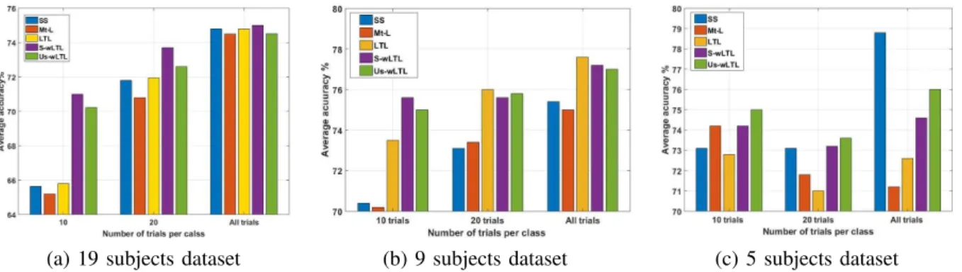
Fig. 1 presents the classification results of the different algorithms when 10, 20 and all subject-specific training trials per class were available from the new target subject. As shown in Fig. 1(a) all the proposed transfer learning algorithms outperformed SS and Mt-L algorithms when 10 and 20 trials per class were available for training whereas, only S-wLTL outperformed the baseline algorithms when all trials were available for training. Specifically, the improvement was more pronounced when only 10 subject-specific trials per class were available for training. However, in Fig. 1(b) all the proposed transfer learning algorithms outperformed SS and Mt-L algorithms across all the above-mentioned different num-ber of subject-specific training trials. Again, the improvement was more pronounced when only 10 subject-specific trials were available. Interestingly, on average the proposed weighed transfer learning algorithms when only 10 trials per class were available for training outperformed the subject-specific algorithm when all trials were available for training. These outcomes support our aim to reduce the calibration time and at the same time increase the classification accuracy.
Learning from few examples typically leads to an ill-posed optimization problem. That was why we applied transfer learning to overcome this problem when only few trials were available for training. Since dataset 3 contains only data from 5 subjects, transfer learning had been done using only the available data from 4 subjects. As shown in Fig. 1(c), despite having such a small pool of data for transfer learning, the proposed transfer learning algorithms still had superior results compared to the baseline algorithms when a few subject-specific trials were available for training. When only 10 training trials per class were available from the new subject, Us-wLTL outperformed baseline algorithms while S-wLTL outperformed only the SS algorithm. Moreover, when 20 trials
(a) 19 subjects dataset (b) 9 subjects dataset (c) 5 subjects dataset
Fig. 1. Comparison between the average classification accuracy calculated using the proposed logistic transfer learning algorithms (LTL, S-wLTL, and Us-wLTL) and the baseline algorithms (SS and Mt-L) when 10, 20, and all trials per class were available for training from the new subjects. From left to right, the sub-figures present the classification results of a) dataset 1, b) dataset 2, and c) dataset 3 respectively. This figure shows that the proposed S-wLTL and Us-wLTL algorithms outperformed the baseline algorithms, particularly when a small number of subject-specific train trials from the target subject, and/or a medium to large number of previously recorded sessions from different subjects were available.
per class were available for training from the new subject, both of the proposed S-wLTL and Us-wLTL outperformed the baseline algorithms. Increasing the number of subject-specific training trials from the new subject led to a decrease in the improvement, such that the SS algorithm outperformed the proposed transfer learning algorithms when all subject-specific trials (i.e. 80 trials) were available. Thus, with larger amounts of target training data, transfer learning became ineffective.
Concerning statistical significance, the Shapiro-Wilk test was used to make sure that our classification accuracy results were normally distributed. Based on the Shapiro-Wilk test re-sults, we rejected the alternative hypothesis and concluded that our classification results came from a normal distribution and hence ANOVA test could be used to compare the classification accuracy between different algorithms at a different number of trials. A 3 (Number of trials)×5 (Algorithms) repeated measure ANOVA test was performed on the results of each dataset separately followed by post-hoc analyses. For dataset 1 Statistical results revealed that using different algorithms had a main effect on the classification accuracy with (P=0.001). Based on the post-hoc analysis, S-wLTL (Us-wLTL) signif-icantly outperformed SS and Mt-L with the P values equal to 0.001 and 0.0001 (0.011 and 0.003) respectively. Similarly, for dataset 2, the use of different algorithms also had a main effect on the classification accuracy with (P = 0.035). Based on the post-hoc analysis, S-wLTL (Us-wLTL) significantly outperformed SS and Mt-L with the P values equal to 0.031 and 0.025 (0.035 and 0.04) respectively. Finally, for dataset 3, as expected, there was no significant difference between any of the proposed and the baseline algorithms.
Another comparison was done where results from the three datasets were combined together. A 3 (Number of trials)×5 (Algorithms) repeated measure ANOVA test was conducted. Results showed that using different algorithms significantly affected the classification accuracy with P=0.0001. Post-hoc multiple comparisons revealed that S-wLTL was significantly better than SS and Mt-L with P values of 0.002 and 0.001 respectively. Besides, Us-wLTL was significantly better than SS, and Mt-L with P-values of 0.032 and 0.01 respectively. Moreover, there was no significant difference between Mt-L and SS.
TABLE II
OVERVIEW OF THE RESULTS WHEN10TRIALS PER CLASS WERE
AVAILABLE FOR TRAINING FROM THE NEW SUBJECT. GROUPING WAS
PERFORMED BASED ONSSERROR RATE.
Error Rate 0-10 10-30 >30 SS (Mean) 93.3 80 57.9 Mt-L (Mean) 87 81.7 56.4 S-wLTL(Mean) 94 85.8 62.2 Us-wLTL(Mean) 93.5 86 61.4 p−value(SS versus S-wLTL) 0.5 0.01 0.023
p−value(SS versus Us-wLTL) 0.5 0.003 0.038
p−value(Mt-L versus S-wLTL) 0.258 0.069 0.003
p−value(Mt-L versus Us-wLTL) 0.314 0.056 0.004
To gain a better insight into the performance of the proposed weighted transfer learning algorithms, the subjects from all datasets were categorized to three groups based on their error rates obtained using the SS algorithm. Table II presents the results when 10 subject-specific trials per class were available for training. The first four rows of this table compare the average classification accuracies of the different groups obtained by the baseline algorithms (SS, and Mt-L) and the proposed weighted transfer learning algorithms (S-wLTL, and Us-wLTL) respectively. As shown in these four rows, both S-wLTL and Us-S-wLTL outperformed the baseline algorithms in all the three groups. Subsequently, the last four rows show the statistical paired t-test results between the baseline and the proposed weighted transfer learning algorithms for the different groups. As shown in the fifth and sixth rows, the proposed weighted transfer learning algorithms were more effective when the error rate obtained by the SS algorithm was medium and high. On the other side, the subjects who performed well with the SS algorithm benefited less from applying the proposed transfer learning approach. This makes sense since these subjects already have well-separated features obtained using the standard CSP filters and the subject-specific classifier. Thus, there is not that much room for improvement of the performance for these subjects. In contrast, changing the classifier parameters through the proposed transfer learning approach improved the accuracy of the subjects with poor and medium BCI performance. Finally, the last two rows of Table II show that there was a significant difference between Mt-L
and the proposed algorithms for poor subject-specific BCI per-formance and tends to be significant with medium perper-formance subjects. Again, there was no significant difference between Mt-L and any of the proposed weighted algorithms at the low error rate.
V. DISCUSSION
The KL divergence measurement requires estimation of the covariance matrices. The estimation of the covariance matrices could be very inaccurate when only few EEG trials are available [45] as those few trials may not well represent the entire distribution of the data. Despite this limitation, our results showed that even using a few trials from the target subjects the proposed KL-based weights were successful in enhancing the classification accuracy. To further improve the classification results, in the future work, we aim to improve the estimation of the KL divergence in the proposed similarity weight formula by applying robust methods of estimating the covariance matrices (such as [46] where the negative impact of having few trials are mitigated).
Another issue to discuss is the use of the power of 4 for KL in (9). In fact, in (9), power 4 was applied on KL rather than power 1 to increase sparsity between similarity weights and to give larger weights to subjects with similar feature distributions and smaller weights to subjects with dissimilar features. In a number of random investigations, we noticed when using the power of 1, fairly similar weights were obtained for many different subjects. Subsequently, compared to LTL, the proposed Sw-LTL algorithm with KL power of 1 did not yield better results. On the other hand, the S-wLTL classification results were greatly enhanced when KL power was increased to 4 in (9). For example, in dataset 2, when only 10 subject-specific trials per class were available, the Sw-LTL algorithm with the KL power of 4 significantly outperformed the Sw-LTL algorithm with the KL power of 1 by an average of 2.6% (p=0.0478). Future work could be extended to estimate the optimum KL power for each subject individually.
Regarding the calibration and computational complexity, the time required for collecting the calibration trials was reduced from around 15 minutes when using the trials of a full session to 2.83 minutes when using only 10 trials per class for training. In order to compare the proposed algorithms and SS from the computational time point of view, we need to note that the proposed algorithms can be divided into two parts. The first part, where the classification parameters of the previous subjects and share priors are calculated using equations (2) to (7), can be done offline without using any data from the target subject. The second part, where the classification parameters of the target subject are calculated using the few available trials of the target subject and the previous subjects shared priors (i.e. µw,ΣT L w) needs to be done online. This part
is the part that should be compared to the SS algorithm in terms of computational time. This computation time was considerably incomparable with the time needed for collecting calibration trials. Using MATLAB 2016b and an Intel Core i5-6500 CPU @ 3.20 GHz, the proposed algorithm required 0.14
sec more time for training the classification model compared to the SS algorithm. Thus, in summary, compared to the SS algorithm, the proposed approach remarkably reduced the calibration time, while it just required extra 0.14 S to train the classification model.
In summary, our results suggested that the proposed S-wLTL and Us-S-wLTL could improve the classification accuracy particularly when a small subject-specific training data was available. Importantly, when there were sufficient previously recorded subjects/sessions available, the proposed S-wLTL and Us-wLTL algorithms not only reduced the required calibration time but also for many subjects they enhanced the classi-fication accuracy. The classiclassi-fication results obtained by S-wLTL and Us-S-wLTL were on average very similar. However, the main advantage of Us-wLTL against S-wLTL was that Us-wLTL did not need any labeled data for calculating the weights.
VI. CONCLUSION
This paper proposed a novel weighted transfer learning approach on classification domain to improve MI-based BCI systems. Our results suggested that applying the proposed weighted transfer learning algorithms could lead to reducing the calibration time to 10 trials per class with significantly less sacrifice in the average accuracy of the MI-BCI systems. The results obtained showed that the proposed weighted algorithms significantly outperformed subject-specific BCI algorithm and the multi-task learning algorithm.
Interestingly, the proposed weighted transfer learning al-gorithms yielded a remarkable increase in the classification accuracy for most of the subjects that initially performed BCI with poor or medium accuracy. However, the observed improvement for a few subjects with initially low BCI perfor-mance was not pronounced. It was shown that changing the parameters of classifiers for these subjects was not effective since their feature spaces for different classes were not sepa-rable. These findings suggest that to increase the accuracy of these subjects with poor subject-specific BCI, transfer learning approaches should be applied in a different domain before the classification domain.
The proposed transfer learning approach is not limited to the logistic regression classifier. It can be applied on any classifier with a mathematically defined objective function. Moreover, in this paper similarity weights were calculated using KL-divergence as a similarity measurement. It is good to note that in the future other similarity measures could be used and their performance could be compared to what we proposed.
REFERENCES
[1] J. R. Wolpaw, N. Birbaumer, D. J. McFarland, G. Pfurtscheller, and T. M. Vaughan, “Brain–computer interfaces for communication and control,”
Clinical Neurophysiology, vol. 113, no. 6, pp. 767–791, 2002. [2] E. A. Curran and M. J. Stokes, “Learning to control brain activity: a
review of the production and control of EEG components for driving brain–computer interface (BCI) systems,”Brain and Cognition, vol. 51, no. 3, pp. 326–336, 2003.
[3] E. Niedermeyer and F. L. da Silva, Electroencephalography: basic principles, clinical applications, and related fields. Lippincott Williams & Wilkins, 2005.
[4] F. Lotte, L. Bougrain, and M. Clerc, “Electroencephalography (EEG)-based brain–computer interfaces,”Wiley Encyclopedia of Electrical and Electronics Engineering, pp. 1–20, 2015.
[5] G. Pfurtscheller and F. L. Da Silva, “Event-related EEG/MEG synchro-nization and desynchrosynchro-nization: basic principles,”Clinical Neurophysi-ology, vol. 110, no. 11, pp. 1842–1857, 1999.
[6] M. Arvaneh, C. Guan, K. K. Ang, and C. Quek, “Optimizing spatial fil-ters by minimizing within-class dissimilarities in electroencephalogram-based brain–computer interface,”IEEE Transactions on Neural Networks and Learning Systems, vol. 24, no. 4, pp. 610–619, 2013.
[7] F. Lotte, “Signal processing approaches to minimize or suppress cal-ibration time in oscillatory activity-based brain–computer interfaces,”
Proceedings of the IEEE, vol. 103, no. 6, pp. 871–890, 2015. [8] S. Saha, K. I. U. Ahmed, R. Mostafa, L. Hadjileontiadis, and A.
Khan-doker, “Evidence of variabilities in EEG dynamics during motor imagery-based multiclass brain–computer interface,”IEEE Transactions on Neural Systems and Rehabilitation Engineering, vol. 26, no. 2, pp. 371–382, 2018.
[9] M. Krauledat, M. Schr¨oder, B. Blankertz, and K.-R. M¨uller, “Reducing calibration time for brain-computer interfaces: A clustering approach,” inAdvances in Neural Information Processing Systems, 2007, pp. 753– 760.
[10] W. Tu and S. Sun, “A subject transfer framework for EEG classification,”
Neurocomputing, vol. 82, pp. 109–116, 2012.
[11] A. M. Azab, J. Toth, L. S. Mihaylova, and M. Arvaneh, “A review on transfer learning approaches in brain–computer interface,” inSignal Processing and Machine Learning for Brain-Machine Interfaces. The Institution of Engineering and Technology (IET), 2018, ch. 5. [12] S. J. Pan and Q. Yang, “A survey on transfer learning,”IEEE
Transac-tions on Knowledge and Data Engineering, vol. 22, no. 10, pp. 1345– 1359, 2010.
[13] S. J. Pan, Q. Yang et al., “A survey on transfer learning,” IEEE Transactions on knowledge and data Engineering, vol. 22, no. 10, pp. 1345–1359, 2010.
[14] Y. Li, H. Kambara, Y. Koike, and M. Sugiyama, “Application of co-variate shift adaptation techniques in brain–computer interfaces,”IEEE Transactions on Biomedical Engineering, vol. 57, no. 6, pp. 1318–1324, 2010.
[15] P. Zanini, M. Congedo, C. Jutten, S. Said, and Y. Berthoumieu, “Transfer learning: a riemannian geometry framework with applications to brain– computer interfaces,”IEEE Transactions on Biomedical Engineering, vol. 65, no. 5, pp. 1107–1116, 2018.
[16] I. Hossain, A. Khosravi, and S. Nahavandhi, “Active transfer learning and selective instance transfer with active learning for motor imagery based BCI,” inProceedings of International Joint Conference on Neural Networks (IJCNN). IEEE, 2016, pp. 4048–4055.
[17] I. Hossain, A. Khosravi, I. Hettiarachchi, and S. Nahavandi, “Multiclass informative instance transfer learning framework for motor imagery-based brain-computer interface,”Computational Intelligence and Neu-roscience, 2018.
[18] H. Kang, Y. Nam, and S. Choi, “Composite common spatial pattern for subject-to-subject transfer,”IEEE Signal Processing Letters, vol. 16, no. 8, pp. 683–686, 2009.
[19] W. Samek, F. C. Meinecke, and K.-R. M¨uller, “Transferring subspaces between subjects in brain–computer interfacing,”IEEE Transactions on Biomedical Engineering, vol. 60, no. 8, pp. 2289–2298, 2013. [20] F. Lotte and C. Guan, “Learning from other subjects helps reducing
brain-computer interface calibration time,”In Proceedings of ICASSP, IEEE International Conference on Acoustics, Speech and Signal Pro-cessing, pp. 614–617, 2010.
[21] W. Samek, M. Kawanabe, and K.-R. M¨uller, “Divergence-based frame-work for common spatial patterns algorithms,”IEEE Reviews in Biomed-ical Engineering, vol. 7, pp. 50–72, 2014.
[22] C. Vidaurre, M. Kawanabe, B. Blankertz, K. M¨uller et al., “Toward unsupervised adaptation of LDA for brain-computer interfaces.”IEEE Transactions on Biomedical Engineering, vol. 58, no. 3, pp. 587–597, 2011.
[23] C. Vidaurre, A. Schlogl, R. Cabeza, R. Scherer, and G. Pfurtscheller, “Study of on-line adaptive discriminant analysis for EEG-based brain computer interfaces,”IEEE Transactions on Biomedical Engineering, vol. 54, no. 3, pp. 550–556, 2007.
[24] P. Shenoy, M. Krauledat, B. Blankertz, R. P. Rao, and K.-R. M¨uller, “To-wards adaptive classification for BCI,”Journal of Neural Engineering, vol. 3, no. 1, p. R13, 2006.
[25] S. Fazli, F. Popescu, M. Dan´oczy, B. Blankertz, K.-R. M¨uller, and C. Grozea, “Subject-independent mental state classification in single trials,”Neural networks, vol. 22, no. 9, pp. 1305–1312, 2009.
[26] M. Alamgir, M. Grosse-Wentrup, and Y. Altun, “Multitask learning for brain-computer interfaces,”Proceedings of the Thirteenth International Conference on Artificial Intelligence and Statistics (AISTATS-10), vol. 9, pp. 17–24, 2010.
[27] V. Jayaram, M. Alamgir, Y. Altun, B. Scholkopf, and M. Grosse-Wentrup, “Transfer learning in brain-computer interfaces,”IEEE Com-putational Intelligence Magazine, vol. 11, no. 1, pp. 20–31, 2016. [28] N. M. Nasrabadi, “Pattern recognition and machine learning,”Journal
of Electronic Imaging, vol. 16, no. 4, p. 049901, 2007.
[29] S. Shalev-Shwartz and A. Tewari, “Stochastic methods for l1-regularized loss minimization,”Journal of Machine Learning Research, vol. 12, no. Jun, pp. 1865–1892, 2011.
[30] C. Robert, “Machine learning, a probabilistic perspective,” 2014. [31] J. Shore and R. Johnson, “Axiomatic derivation of the principle of
maximum entropy and the principle of minimum cross-entropy,”IEEE Transactions on Information Theory, vol. 26, no. 1, pp. 26–37, 1980. [32] M. R. Hestenes and E. Stiefel, Methods of conjugate gradients for
solving linear systems, 1952, vol. 49, no. 1.
[33] I. Iturrate, L. Montesano, and J. Minguez, “Task-dependent signal variations in EEG error-related potentials for brain–computer interfaces,”
Journal of Neural Engineering, vol. 10, no. 2, p. 026024, 2013. [34] B.-C. Kuo and D. A. Landgrebe, “Nonparametric weighted feature
extraction for classification,” IEEE Transactions on Geoscience and Remote Sensing, vol. 42, no. 5, pp. 1096–1105, 2004.
[35] M. Arvaneh, C. Guan, K. K. Ang, T. E. Ward, K. S. Chua, C. W. K. Kuah, G. J. E. Joseph, K. S. Phua, and C. Wang, “Facilitating motor imagery-based brain–computer interface for stroke patients using passive movement,”Neural Computing and Applications, vol. 28, no. 11, pp. 3259–3272, 2017.
[36] M. Naeem, C. Brunner, R. Leeb, B. Graimann, and G. Pfurtscheller, “Seperability of four-class motor imagery data using independent com-ponents analysis,”Journal of neural engineering, vol. 3, no. 3, p. 208, 2006.
[37] C. Brunner, R. Leeb, G. M¨uller-Putz, A. Schl¨ogl, and G. Pfurtscheller, “BCI competition 2008–Graz data set A,” Institute for Knowledge Discovery (Laboratory of Brain-Computer Interfaces), Graz University of Technology, 2008.
[38] G. Dornhege, B. Blankertz, G. Curio, and K.-R. Muller, “Boosting bit rates in noninvasive EEG single-trial classifications by feature combi-nation and multiclass paradigms,” IEEE Transactions on Biomedical Engineering, vol. 51, no. 6, pp. 993–1002, 2004.
[39] F. Lotte and C. Guan, “Regularizing common spatial patterns to improve bci designs: Unified theory and new algorithms,”IEEE Transactions on Biomedical Engineering, vol. 58, no. 2, pp. 355–362, 2011.
[40] H. Ramoser, J. Muller-Gerking, and G. Pfurtscheller, “Optimal spatial filtering of single trial EEG during imagined hand movement,” IEEE Transactions on Rehabilitation Engineering, vol. 8, no. 4, pp. 441–446, 2000.
[41] F. Lotte and C. Guan, “Learning from other subjects helps reducing brain-computer interface calibration time,” in In proceedings of IEEE International Conference on Acoustics Speech and Signal Processing (ICASSP), 2010. IEEE, 2010, pp. 614–617.
[42] B. Blankertz, R. Tomioka, S. Lemm, M. Kawanabe, and K.-R. Muller, “Optimizing spatial filters for robust eeg single-trial analysis,” IEEE Signal processing magazine, vol. 25, no. 1, pp. 41–56, 2008. [43] F. Lotte, M. Congedo, A. L´ecuyer, F. Lamarche, and B. Arnaldi,
“A review of classification algorithms for eeg-based brain–computer interfaces,”Journal of neural engineering, vol. 4, no. 2, p. R1, 2007. [44] K.-H. Fiebig, V. Jayaram, J. Peters, and M. Grosse-Wentrup,
“Multi-task logistic regression in brain-computer interfaces,” in Proceedings of IEEE International Conference on Systems, Man, and Cybernetics (SMC). IEEE, 2016, pp. 002 307–002 312.
[45] Y. Guo, “Regularized discriminant analysis and its application in mi-croarrays,”Biostatistics, vol. 1, no. 1, pp. 1–18, 2005.
[46] X. Yong, R. K. Ward, and G. E. Birch, “Robust common spatial patterns for EEG signal preprocessing,” in30th Annual International Conference of the Engineering in Medicine and Biology Society, IEEE, 2008. EMBS 2008. IEEE, 2008, pp. 2087–2090.