SFB 649 Discussion Paper 2005-026
Projection Pursuit for
Exploratory Supervised
Classification
Eun-Kyung Lee*
Dianne Cook*
Sigbert Klinke**
Thomas Lumley***
* Department of Statistics, Iowa State University, USA ** Institute for Statistics and Econometrics,
Humboldt-Universität zu Berlin, Germany
*** Department of Biostatistics, University of Washington, USA
This research was supported by the Deutsche
Forschungsgemeinschaft through the SFB 649 "Economic Risk". http://sfb649.wiwi.hu-berlin.de
ISSN 1860-5664
SFB 649, Humboldt-Universität zu Berlin Spandauer Straße 1, D-10178 Berlin
S
FB
6
4
9
E
C
O
N
O
M
I
C
R
I
S
K
B
E
R
L
I
N
Projection Pursuit for
Exploratory Supervised Classification
0
EUN-KYUNG LEE1, DIANNE COOK2, SIGBERT KLINKE3, and THOMAS LUMLEY41 Department of Statistics, Ewha Womans University 2 Department of Statistics, Iowa State University
3 Institute for Statistics and Econometrics, Humboldt-Universit¨at zu Berlin 4 Department of Biostatistics, University of Washington
ABSTRACT
In high-dimensional data, one often seeks a few interesting low-dimensional projections that reveal important features of the data. Projection pursuit is a procedure for searching high-dimensional data for interesting low-dimensional projections via the optimization of a criterion function called the projection pursuit index. Very few projection pursuit indices incorporate class or group information in the calculation. Hence, they cannot be adequately applied in supervised classification problems to provide low-dimensional projections revealing class differences in the data . We introduce new indices derived from linear discriminant analysis that can be used for exploratory supervised classification.
Key Words:
Data mining; Exploratory multivariate data analysis; Gene expression data; Discriminant analysis;0This research was supported by the Deutsche Forschungsgemeinschaft through the SFB 649 Economic Risk.
1. Introduction
This paper is about methods for finding interesting projections of multivariate data when the observations belong to one of several known groups. The type of data is denoted as ap-dimensional vectorXij representing
thejth observation of theith class,i= 1, . . . , g,gis the number of classes,j= 1, . . . , ni, andniis the number
of observations in class i. Let ¯Xi. =Pnj=1i Xij/ni be the ith group mean and ¯X.. =Pgi=1Pnj=1i Xij/n be
the total mean, wheren=Pg
i=1ni. Interesting projections correspond to views where there are the biggest
difference between the observations from different classes, that is, the classes are clustered in the view. In this paper, the approach to finding interesting projections uses the measures of between group variation, relative to within-group variation. These new methods are important for exploratory data analysis and data mining purposes when the task is to (1) examine the nature of clustering in the space of the data due to class information, and (2) to build a classifier for predicting the class of new data.
Projection pursuit is a method to search for interesting linear projections by optimizing some pre-determined criterion function, called a projection pursuit index. This idea originated with Kruskal (1969), and Friedman and Tukey (1974) first used the term “projection pursuit” describing a technique for ex-ploratory analysis of multivariate data. It is useful for an initial data analysis, especially when data is in a high dimensional space. A problem many multivariate analysis techniques face is “the curse of dimen-sionality”, that is, most of high dimensional space is empty. Projection pursuit methods help us explore multivariate data in interesting low dimensional spaces. The definition of an “interesting” projection depends on the projection pursuit index and on the application or purpose.
Many projection pursuit indices have been developed to define interesting projections. Because most low-dimensional projections are approximately normal (Huber, 1985), most of the projection pursuit indices are focused on non-normality. For example, the entropy index and the moment index (Jones and Sibson, 1987), the Legendre index (Friedman, 1987), the Hermite index (Hall, 1989), and the Natural Hermite index (Cook, et al, 1993), all search for projections where the data exhibit a high degree of non-normality.
Visual inspection of high dimensional data using projections is helpful to understand data, especially when it is combined with dynamic graphics. GGobi is an interactive and dynamic software system for data visualization and projection pursuit is implemented in it dynamically (Swayne, et al, 2003). The Holes index and the central mass index in GGobi are helpful in finding projections with few observations in the center and projections containing an abundance of points in the center, respectively (Cook, et al, 1993).
As the data mining area has grown, projection pursuit methods are increasingly used in classification and clustering to escape the curse of dimensionality. Posse (1992) suggested a method for projection pursuit discriminant analysis for two groups. He used kernel density estimation of the projected data instead of the original data and used the total probability of misclassification of the projected data as a projection pursuit index. Polzehl (1995) considered the cost of misclassification and used the expected overall loss as a projection pursuit index. Flick, et al (1990) uses a basis function expansion to estimate density and minimizes a measure of scatter. These projection pursuit methods for classification focus on 1-dimensional projections and it is hard to extend them to k-dimensional projections. Examining higher than 1-dimensional projections is important for visual inspection of high-dimensional data.
The methods presented in this paper start from a well-known classification method called linear discrim-inant analysis(LDA). This approach is extended to provide new projection pursuit indices for exploratory supervised classification. These indices use Fisher’s linear discriminant ideas and expand Huber’s ideas on projection pursuit for classification. These new indices are helpful for building understanding about how class structure relates to measured variables and they can be used to provide graphics to assess and ver-ify supervised classification results. These indices are implemented as an R package, and these indices are available in GGobi for dynamic graphics (Swayne, et al, 2003)
This paper is organized as follows. Section 2 introduces the new projection pursuit indices and describes their properties. The optimization method to find the interesting projections is discussed in Section 3. Section 4 describes how to apply these indices using two gene expression data sets.
2. Index Definition
2.1 LDA projection pursuit index
The first index is derived from classical linear discriminant analysis (LDA). The approach, first developed by Fisher (1938), finds linear combinations of the data which have large between-group sums of squares relative to within-group sums of squares. (For detailed explanations, see Johnson and Wichern, 2002 and Duda et al. 2001) Let
B =
g
X
i=1
ni( ¯Xi.−X¯..)( ¯Xi.−X¯..)T : between-group sums of squares, (1)
W = g X i=1 ni X j=1
(Xij−X¯i.)(Xij−X¯i.)T : within-group sums of squares. (2)
Dimension reduction is achieved by finding the linear projection,a, that maximizes (aTBa)/(aTWa), which leads to the natural definition of a projection pursuit index. (aTBa)/(aTWa) ranges between 0 and 1, where low values correspond to projections that display little class difference and high values correspond to projections that have large differences between the classes. To extend to an arbitrary-dimensional projection, we consider a test statistic used in multivariate analysis of variance (MANOVA) called Wilks Λ∗=W
/
W+ B. This quantity also ranges between 0 and 1, although the interpretation of numerical values are reversed from the 1-dimensional measure defined above. Small values of Λ∗ correspond to large differences between
the classes.
LetA= [a1a2 · · · ak] define an orthogonal projection onto ak-dimensional space. In projection pursuit
the convention is that interesting projections are the ones that maximize the projection pursuit index, so we use the negative value of Wilks Lambda and add 1 to keep this index between 0 and 1. This gives the LDA projection pursuit index (LDA index) as:
ILDA(A) = 1− A T WA AT W+BA forA T W+BA6= 0 0 forA T W+BA= 0 (3)
Low index values correspond to little difference between classes and high values correspond to large differences between classes. The next proposition quantifies the minimum and maximum values. For simplicity, we denoteW+B as Φ.
Proposition 1. Let rank(Φ) = p, k≤min(p, g). Then, 1− k Y i=1 λi≤ILDA(A)≤1− p Y i=p−k+1 λi (4) where λ1,≥λ2≥ · · · ≥λp≥0 : eigenvalues ofΦ−1/2WΦ−1/2, e1,e2,· · · ,ep : corresponding eigenvectors of Φ−1/2WΦ−1/2, f1,f2,· · · ,fp : eigenvectors of Φ−1/2BΦ−1/2.
In (4), the right equality holds whenA=Φ−1/2[ep ep−1 · · · ep−k+1] =Φ−1/2[f1 f2 · · · fk] and the
left equality holds whenA=Φ−1/2[ek ek−1 · · · e1] =Φ−1/2[fp−k+1 fp−k+2 · · ·fp].
A problem arises for LDA when rank(W) = r < p. We need to remove collinearity by removing vari-ables, before applying LDA. Otherwise, we need to modify the W−1 calculation, for example, to use the pseudo-inverse (pseudo LDA : Fukunaga, 1990) , or to use a ridge estimate instead of W such as regu-larized discriminant analysis (Friedman, 1989). For projection pursuit, because we make calculations in k-dimensional space instead of p-dimensional space, we can find interesting projections without an initial dimension reduction or modifiedWcalculation. The next proposition shows how the LDA index works when rank(W)< p.
Proposition 2. Let rank(Φ) = r < p, k≤min(r, g). Then, 1− k Y i=1 δi≤ILDA(A)≤1− r Y i=r−k+1 δi (5)
where Φ= P Q Λ 0 0 0 PT QT =PΛPT : spectral decomposition of Φ, P:k×rmatrix,PTP=Ir, Q:k×(k−r) matrix,QTQ=Ik−r,
Λ= diag[δ1, δ2,· · · , δr] :r×rdiagonal matrix,
δ1, δ2,· · ·, δr: eigenvalues ofΛ−1/2PTWPΛ−1/2,
e1,e2,· · · ,er : corresponding eigenvectors ofΛ−1/2PTWPΛ−1/2.
In (5), the right equality holds whenA=PΛ−1/2[e
r er−1 · · · er−k+1], and the left equality holds
whenA=PΛ−1/2[e k ek−1 · · · e1]. (b) (c) (a) 1D projected data −2 −1 0 1 2 0 5 10 15 20 25 30 35 (b) 1D projected data −4 −3 −2 −1 0 1 2 3 0 5 10 15 20 25 30 (c)
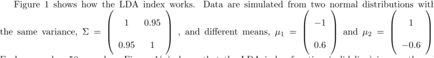
Figure 1. (a) Huber’s plot(1990) usingILDAon data simulated from two bivariate normal population. The symbols
and +represent two different classes. The solid ellipse representsILDA value for all 1-dimensional projections,
and the dashed circle is a guide set at the medianILDA value. The straight dotted line labelled (b) is the optimal
projection direction usingILDA and the histogram of the projected data is shown in the correspondingly labelled plot
(b). In plot (a) the dotted line labelled (c) is the first principal component direction and the the histogram of the
projected data is shown in the correspondingly labelled plot(c).
index (Figure 1), we use a type of plot that was introduced by Huber (1990). In one-dimensional projections from a 2-dimensional space, forθ= 0◦,· · ·,179◦, the projection pursuit index is calculated using projection
aθ= (cosθ, sinθ) and displayed radially as a function ofθ. In each figure, the data points are plotted in the
center. The solid ellipse represents the index value, ILDA, plotted at distances relative to the center. The
dotted circle is a guide line plotted at the median index value.
Figure 1 shows how the LDA index works. Data are simulated from two normal distributions with
the same variance, Σ = 1 0.95 0.95 1
, and different means, µ1 =
−1 0.6 and µ2 = 1 −0.6 .
Each group has 50 samples. Figure 1(a) shows that the LDA index function (solid line) is smooth and has a maximum value when the projected data reveals two separated classes. Figure 1(b) and Figure 1(c) are the histograms of the optimal projected data using the LDA index and the data projected onto the first principal component. The LDA index finds separated class structure. Principal component analysis is commonly used to find revealing low-dimensional projections, but it really does not work well in classification problems. Here, principal component analysis solves a different problem: It finds a projection that shows large variation (Johnson and Wichern, 2002).
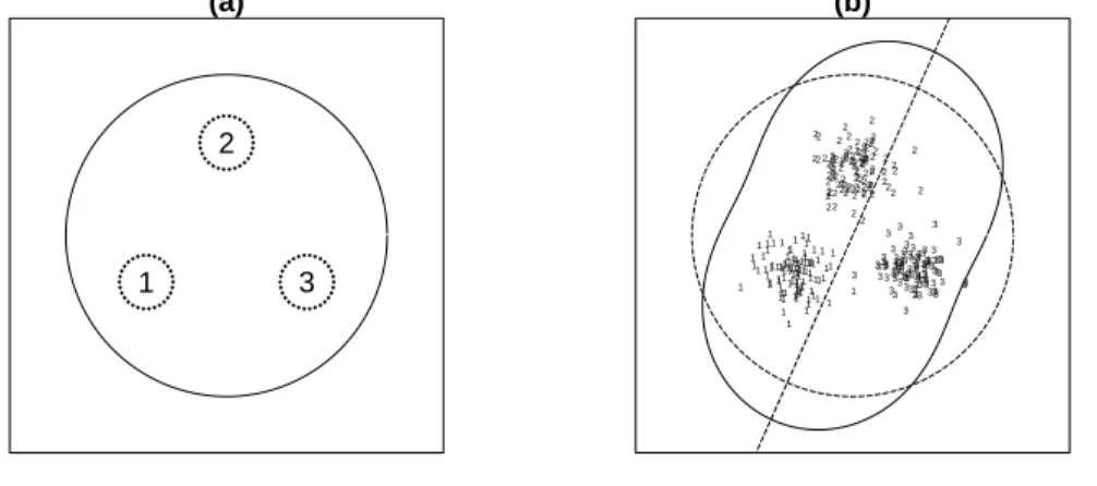
The LDA index works well generally, but it has some problems in special circumstances. One special situation is 2-dimensional data generated from a uniform mixture of three Gaussian distributions, with identity variance-covariance matrices and centers at the vertices of an equilateral triangle. Figure 2(a) shows the theoretical case where three classes have the exact same variance-covariance matrix and three class means are the vertices of an equilateral triangle. In this case, all directions have the same LDA index values. The best projection is the full 2-dimensional data space. Figure 2(b) shows data simulated from this distribution. Because of the sampling, variances are slightly different in each class and the three means do not lie exactly on an equilateral triangle. Therefore the optimal direction(the dotted straight line in Figure 2(b)) depends on the sampling variation. If a new sample is generated, a completely different optional projection will occur. This is not what we want in exploratory methods. We would like to be able to find all the interesting data
structures, which in this case would be the three 1-dimensional projections revealing each group separated from the other two groups. We extend this problem of the LDA index to define a new index that is able to detect interesting structures in this situation.
2.2 LDA extended projection pursuit index using
L
r-norm
We start from the 1-dimensional index. Letyij=aTXij be a projected observation onto a 1-dimensional
space. In the LDA index, we use aTBaand aTWa as the measures of between-group and within-group
variations, respectively. These two measures can be explained as the square ofL2 vector norm, as follows.
1 3 2 (a) 1 1 111 1 1 1 1 1 1 1 1 1 111 1 1 1 1 1 1 1 1 1 1 1 1 1 1 1 1 1 1 1 1 1 1 1 1 1 1 1 1 1 1 1 1 1 1 1 1 1111 1 1 1 1 1 1 1 1 1 1 1 1 11 1 1 1 1 1 1 1 1 1 1 1 1 1 1 1 1 1 1 1 1 1 1 1 1 1 1 1 1 1 3 3 3 3 3 3 3 3 3 3 3 3 3 3 33 3 3 3 33 3 33 3 3 3 3 3 3 3 33 3 3 3 3 3 3 3 3 3 33 3 3 3 3 3 3 3 3 3 3 3 3 3 3 3 3 3 3 3 3 3 3 3 3 3 3 3 3 33 3 3 3 3 33 3 3 3 3 3 3 3 3 3 3 3 33 3 3 3 3 3 3 3 2 2 2 2 2 2 2 2 2 2 2 2 2 2 2 2 2 2 2 2 2 2 2 2 2 2 2 2 2 2 2 2 2 2 2 2 2 2 2 2 2 2 2 2 2 2 2 2 2 2 2 2 2 2 2 2 2 2 2 22 2 2 2 2 2 2 2 2 2 2 2 22 2 2 2 2 2 2 2 2 2 2 2 2 2 2 2 2 2 2 2 2 22 2 2 2 2 (b)
Figure 2. This plot illustrates a problem situation for ILDA. (a) The theoretical case where the three classes
have the exact same variance and the three class means come are located on the vertices of an equilateral triangle.
All directions have exactly same ILDA values (solid circle). The best projection is really the full 2-dimensional data
space! (b) What happens in practice? This plot contains data generated from the theoretical distribution. An optimal projection is found purely due to sampling variation. If a new sample were generated a completely different optimal projection will be found.
aTBa = g X i=1 ni X j=1 (¯yi.−y¯..) 2 =||My¯g−1ny¯..||2 2 (6) aTWa = g X i=1 ni X j=1 (yij−y¯i.) 2 = ||y−My¯g||2 2 (7) aTΦa = g X i=1 ni X j=1 (yij−y¯..) 2 ={||y−1ny¯..||2} 2 =||My¯g−1ny¯..||2 2 +||y−My¯g||2 2 (8) whereM=diag(1n1,· · · ,1ng), ¯yg= [¯y1.,y¯2.,· · ·,y¯g.] T , y=y1T,y2T,· · ·,ygT T , yi= yi1, yi2,· · ·, ying T , and1n= [1,1,· · · ,1] T
: n×1 vector. We extend to theLr norm. Let
Br = ||My¯g−1ny¯..||r r = g X i=1 ni X j=1 |y¯i.−y¯..|r (9) Wr = ||y−M¯yg||r r = g X i=1 ni X j=1 |yij−y¯i.|r. (10) Then {||y−1ny¯..||r} r = g X i=1 ni X j=1 |yij−y¯..|r ≤ g X i=1 ni X j=1 |y¯i.−y¯..|r+ g X i=1 ni X j=1 |yij−y¯i.|r=Br+Wr. (11)
Even though the additivity does not hold for the Lr vector norm, Br and Wr can be substitutes for the
measures of between-group and within-group variabilities. We use these measures to define our new index. The 1-dimensionalLrprojection pursuit index (Lr index) is defined by
ILr(a) = Br Wr 1/r = ||My¯g−1ny¯..||r ||y−M¯yg||r (12) = Pg i=1 Pni j=1(¯yi.−y¯..) r Pg i=1 Pni j=1(yij−y¯i.) r !1/r . (13)
Taking the ratio to the 1/r power, prevents this index value from getting too big. The 1-dimensional LDA index is a special case of this index whenr= 2.
For a k-dimensional projection A, letYij =ATXij = [yij1, yij2,· · · , yijk] T
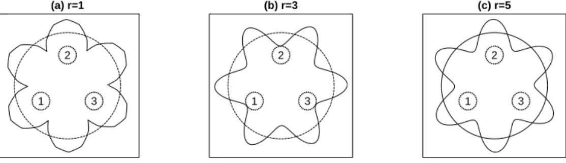
1 3 2 (a) r=1 1 3 2 (b) r=3 1 3 2 (c) r=5
Figure 3. Huber’s plot showing behavior ofILr index on the special data that caused problems forILDA. (a) IL1:
The optimal projections separate each class from the other two. (b) IL3: The optimal projections separate all three
classes. (c)IL5: The optimal projections separate each class from the other two. When r=2 and r=4, the index is
the same asILDA, shown in Figure 2(a).
onto thek dimensional space spanned byA. Then [ATBA]lm = g X i=1 ni X j=1 (¯yi.l−y¯..l) (¯yi.m−y¯..m), (14) [ATWA]lm = g X i=1 ni X j=1
(yijl−y¯i.l) (yijm−y¯i.m) (15)
wherel, m= 1,2,· · ·, k. The diagonals of these matrices represent the variances of the between (or within) group for each variable and the off-diagonals represent covariances between variables. We take only the diagonal parts of these between-group and within-group variance and extend these sums of squares to Lr
norms. Then, ILr(A) = Pk l=1 Pg i=1 Pni j=1(¯yi.l−y¯..l) r Pk l=1 Pg i=1 Pni j=1(yijl−y¯i.l) r !1/r . (16)
For detailed explanations, see Lee (2003).
Figure 3 shows how the new indexILr (r= 1,2,3) performs for the special situation that caused problem
forILDA. When r= 1, all three optimal projections separate one class from the other two classes. When
projections as theL1index but the index function is smoother than theL1index. Whenris 2 and 4, these
indices have the same value for all directions, just like the LDA index.
The LDA index and the Lr index (r≥2) are usually sensitive to outliers, mainly due to use the sums
of squares or higher power, which are sensitive measure to outliers. On the other hand, theL1 index uses
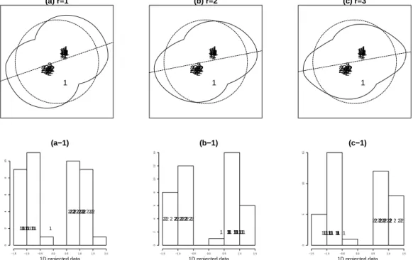
the sums of absolute values. Therefore it is more robust to outliers than other indices. Figure 4 shows how these indices work in the presence of an outlier. In each plot, there are two classes (1 and 2). The class 1 has 21 observations with one outlier and the class 2 has 20 observations. The histogram of the optimal 1-dimensional projected data using the L1 index (Figure 4 (a-1)) shows that the outlier is separated from
two groups and the best projection is not affected by this outlier. When r ≥ 2, the best projections are leveraged towards the direction of the outlier. With the exception of the outlier, the L1 index provides a
more separated view of the two classes than the best projection of theLr(r≥2) index.
1 11 11111 1 111 111111 11 2 2 2 2 22 222 2222222222 2 1 (a) r=1 1 11 11111 1 111111111 11 2 2 2 2 22 222 2222222222 2 1 (b) r=2 111 11111 1 1 11 1 11 111 11 2 2 2 2 22 222 2222222222 2 1 (c) r=3 1D projected data −1.5 −1.0 −0.5 0.0 0.5 1.0 1.5 2.0 02468 1 0 1 111 1 11 1 1 1111111 1111 1 222 22222222 2 2 22 22 2 22 (a−1) 1D projected data −1.5 −1.0 −0.5 0.0 0.5 1.0 1.5 02468 1 0 1 2 1 4 111 1 111 1 1 1 111 111 1 111 1 2 2 2 2222 2222 22222 2222 (b−1) 1D projected data −1.5 −1.0 −0.5 0.0 0.5 1.0 1.5 0 5 10 15 1 111 1 11 111111 11 111111 2 2 2 2 2222 2222 2 22 22 2 22 (c−1)
has an outlier. (a) Huber’s plot of IL1, (a-1) Histogram of the projected data onto the L1 optimal projection (b)
Huber’s plot ofIL2, (b-1) Histogram of the projected data onto theL2optimal projection (c) Huber’s plot ofIL3, (c-1)
Histogram of the projected data onto theL3 optimal projection.
3. Optimization
A good optimization procedure is an important part of projection pursuit. The purpose of projection pursuit optimization is to find all of the interesting projections, not only to find one global maximum, because sometimes the local maximum can reveal unexpectedly interesting data structure. For this reason, the projection pursuit optimization algorithm needs to be flexible enough to find global and local maxima.
Posse (1990) compared the several optimization procedures, and suggest a random search for finding the global maximum of a projection pursuit index. Cook, et al (1995) use a grand tour alternated with a simulated annealing optimization of a projection pursuit index, to creating a continuous stream of projections that are displayed for exploratory visualization of multivariate data. Klein and Dubes (1989) showed that simulated annealing can produce results as good as those obtained by conventional optimization methods and this method performs well for large data sets.
Simulated annealing was first proposed by Kirkpatrick, et al (1983) as a method to minimize objective functions that have many variables. The fundamental idea of simulated annealing is that a re-scaling pa-rameter, called the “temperature”, allows control of the speed of convergence to a minimum value. For an objective functionh(θ), called the “energy”, we start from the initial valueθ0. A value,θ∗ is generated in
the neighborhood ofθ0. Then,θ∗is accepted as a new value with probabilityρ, defined by the temperature
and the energy difference betweenθ0 andθ∗. This probabilityρguards against getting trapped into a local
minimum allowing the algorithm to visit a local minimum and then jump out and explore for other minima. For detailed explanations, see Bertsimas and Tsitsiklis (1993).
tem-peratures, one (Di) is for neighborhood definition, and the other (Ti) is for the probabilityρ. Diis re-scaled
by the predetermined cooling parameter cand Ti is defined by T0/log(i+ 1). Before we start, we need to
choose the cooling parameter,c, and the initial temperature,T0. The cooling parameter,c, determines how
many iterations are needed to converge and whether the maximum is likely to be a local maximum or a global maximum. The initial temperature, T0, also controls the speed of convergence. Even if the cooling
parametercis small, there is a chance that the algorithm will stop before it reaches the peak. Ifc is large, more iterations are needed to get a final value, but this final solution is more likely to be at the peak value, and that it is a global maximum. Therefore this algorithm is quite flexible for finding interesting projections. (For detailed discussion, see Lee, 2003.)
Simulated Annealing Optimization Algorithm for Projection Pursuit
1. Set an initial projection,A0, and calculate the initial projection pursuit index valueI0=I(A0) .
For theith iteration,
2. Generate a projectionAi from NDi(A0),
whereDi=ci,cis the predetermined cooling parameter in the range (0,1),
NDi(A0) ={A:Ais an orthonormal projection with directionA0+DiB, ∀random projectionsB}
3. CalculateIi=I(Ai), ∆Ii=Ii−I0,Ti= log(Ti0+1),
4. SetA0=Ai andI0=Ii with probabilityρ= min
exp∆Ii
Ti
,1and increaseito i+1 Repeat 2-4 until ∆Ii is small.
4. Application
DNA microarray technologies provide a powerful tool for analyzing thousands of genes simultaneously. Comparison of gene expression levels between samples can be used to obtain information about important
genes and their functions. Because microarrays contain a large number of genes on each chip but typically few chips are used, analyzing DNA microarray data usually means dealing with largep, small nchallenges. A recent publication that compares classification methods for gene expression data (Dudoit, et al., 2002) has focused on the classification error. We will use the same data sets to demonstrate the use of new projection pursuit indices.
4.1 Data sets
Leukemia
This data set originated from a study of gene expression in two types of acute leukemias, acute lymphoblastic leukemia(ALL) and acute myeloid leukemia(AML). The data set consists ofn1= 25 cases ofAML andn2= 47 cases of ALL(38 cases of B-cell ALL and 9 cases of T-cell ALL), givingn= 72. After
pre-processing, we havep= 3571 human genes. This data set is available at http://www-genome.wi.mit.edu/mpr and was described by Golub, et al. (1999).
NCI60
This data set consists of 8 different tissue types where cancer was found : n1= 9 cases from breast,n2 = 5 cases from central nervous system(CNS), n3 = 7 cases from colon, n4 = 8 cases from leukemia,
n5 = 8 cases from melanoma, n6 = 9 cases from non-small-cell lung carcinoma(NSCLC), n7 = 6 cases
from ovarian, and n8 = 9 cases from renal, and p=6830 human genes. Missing values are imputed by a
simpleknearest-neighbor algorithm (k= 5). We use these data to show how to use exploratory projection pursuit classification when the number of classes is large. This data set is available at http://genome-www.stanford.edu/sutech/download/nci60/index.html and was described by Ross, et al. (2000).
Standardization and Gene SelectionThe gene expression data were standardized so that each observa-tion has mean 0 and variance 1. For gene selecobserva-tion, we use the ratio of between-group to within-group sums of squares. BW(j) = Pn i=1 Pg k=1I(yi=k)(¯xk,j−x¯.,j)2 Pn i=1 Pg k=1I(yi=k)(xi,j−x¯k,j)2 (17) where ¯x.,j= (1/n)P n i=1xi,j and ¯xk,j = (P n i=1I(yi=k)xi,j)/(P n
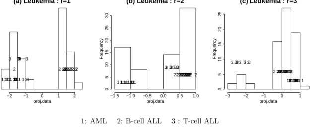
proj.data Frequency −2 −1 0 1 2 0 5 10 15 20 1 1 1 11 1 111111 1 11 11111111 11 2 2 22222 222222 22 2 2 222222 2222 2 2 2222222 22 3 3 3 3 33333 (a) Leukemia : r=1 proj.data Frequency −1.5 −1.0 −0.5 0.0 0.5 1.0 0 5 10 15 20 25 30 1 111 111 1 11 11 1111 111111111 2 2 22 222222 22222 22 2222 22222222222222222 3 3 3 3 33 3 33 (b) Leukemia : r=2 proj.data Frequency −3 −2 −1 0 1 0 5 10 15 20 25 1 1 1 1111 111 11111 11 1 111 1 111 2 2222 2 2222 22 2 22222222 222 22222 222222222 3 3 3 3 3 3333 (c) Leukemia : r=3
1: AML 2: B-cell ALL 3 : T-cell ALL
Figure 5. Leukemia data : 1-dimensional projection (p=40) (a) the histogram of the optimal projected data usingIL1
(b) the histogram of the optimal projected data usingIL2 (c) the histogram of the optimal projected data usingIL3
the original study (Dudoit, et al, 2002) and start with p = 40 for the leukemia data and p= 30 for the NCI60 data and discuss different numbers of genes later.
4.2 Results
1-dimensional projection
Figure 5 displays the histograms of the projected data onto the optimal 1-dimensional projections. For this application, we choose a very large cooling parameter (0.999) which gives us the global maximum. In the Leukemia data, whenr=1 (Figure 5-a), the B-cell ALL class is separated from the other classes except for one case. When r= 2 (Figure 5-b), the three classes are almost separable when theL2 index is used,
which is the same result as for the LDA index. Asris increased, the index tends to separate the T-cell ALL from the others (Figure 5-c).
a
b
Leukemiac
Colond
Renale
Breastf
NSCLC Melanomag
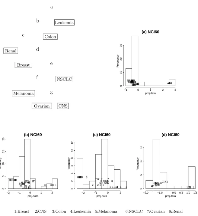
Ovarian CNS proj.data Frequency −1 0 1 2 3 01 0 2 0 3 0 1 1 12222 3332511111153333 44444444 55 55 5 56 6 6 6667667777788 86 8888 8 8 (a) NCI60 proj.data Frequency −2 −1 0 1 2 0 5 10 15 20 1 1122111111 22 2 3 33333 3 5 5 5 5 5655567677666666777 8 8 8 8 888 88 (b) NCI60 proj.data Frequency −2 −1 0 1 02468 1 0 1 2 1 11111 1 1 1 2 2 22 5 5 525 5 555 6 6 6 6 6666 6 77 7 7 7 7 8 8 8 888 8 88 (c) NCI60 proj.data Frequency −2.0 −1.0 0.0 0.5 1.0 1.5 0 5 10 15 1 11 111111 2 2 2225 5 55 5555 6 6 6 6 6 6 6 6 6 77 7777 (d) NCI601:Breast 2:CNS 3:Colon 4:Leukemia 5:Melanoma 6:NSCLC 7:Ovarian 8:Renal
Figure 6. NCI60 data : the 1-dimensional projection (p=30). (a) The histogram of the optimal projection using the LDA index. Leukemia group is separated from the others - peel off Leukemia group. (b)Colon group is separated (c) Renal group is separated (d) Breast group is separated.
many classes. For these data, we try an isolation method that applies projection pursuit iteratively and takes off one class at a time (Friedman and Tukey, 1974). The 8 classes are too many to separate with a single 1-dimensional projection. After finding one split, we apply projection pursuit to each partition. Usually one class is peeled off from the others in each step. The tree diagram in Figure 6 illustrates the steps. In the first step (Figure 6-a), we separate the Leukemia class from the others. At the second step, Colon class is separated (Figure 6-b). Then, the Renal, the Breast, the NSCLC, and the Melanoma classes are separated sequentially. Finally, the Ovarian and the CNS classes are separated.
2-dimensional projection
Figures 7 and 8 show the plot of the data projected onto the optimal 2-dimensional projections for the Leukemia data. All three classes separate easily using the LDA index. Using theL1 index, the B-cell ALL
class is separated with one exception - the same outlier of the result of the 1-dimensional projection in Figure 5(c). In the 2-dimensional case, the LDA index is only the same as theL2 index if Band Ware diagonal
matrices. The best result is obtained using theILDAindex, where all three classes are clearly separated. In
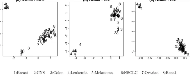
the NCI60 data, the Leukemia class is clearly separated from the others for all indices (Figure 8).
Classification
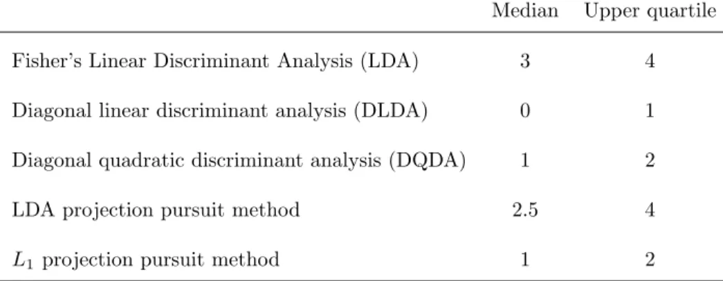
Table 1. Test set error. Median and Upper quartile of the misclassified samples from 200 replications. (ntest= 24)
Median Upper quartile Fisher’s Linear Discriminant Analysis (LDA) 3 4 Diagonal linear discriminant analysis (DLDA) 0 1 Diagonal quadratic discriminant analysis (DQDA) 1 2
LDA projection pursuit method 2.5 4
L1projection pursuit method 1 2
−1.0 −0.5 0.0 0.5 1.0 − 1 01234 2 2 22 222 2 2 2 2 2 2 2 2 2 3 2 2 2 1111 1 11 1 1 11 1 1 1 2 3 3 22 3 2 2 3 3 3 22 3 2 2 2 2 2 2 2 2 3 2 2 2 2 1 1 1 111 1 1 11 1
(a) Leukemia : LDA
−2 −1 0 1 −1.5 −1.0 −0.5 0.0 0.5 1.0 1.5 2 222222 2 2 2 2 22 2 2 2 3 2 2 2 11 1 1 1 1 1 1 1 1 1 1 1 1 2 3 3 2 2 3 2 2 3 3 3 2 2 3 2 2 2 2 222 2 3 2 2 2 2 1 1 1 1 1 1 1 1 1 1 1 (b) Leukemia : r=1 −1.5−1.5 −1.0 −0.5 0.0 0.5 1.0 −1.0 −0.5 0.0 0.5 1.0 2 2 2 2 2 2222 2 2 2 2 2 2 2 3 22 2 11 1 1 1 1 1 1 1 1 1 1 1 1 2 33 22 3 2 2 3 3 3 2 2 3 2 2 2 2 2 2 2 2 3 2 22 2 1 1 1 1 1 1 1 1 1 11 (c) Leukemia : r=2
1: AML 2: B-cell ALL 3 : T-cell ALL
Figure 7. Leukemia data : 2-dimensional projection (p=40). (a) ILDA : The three classes are separated. (b)IL1 :
The B-cell ALL class is separated from the other two except for one case. (c)IL2 : The three classes are separated,
although the gap between classes 2 and 3 is small.
−2 −1 0 1 −1 0 1 2 2 2 2 8 1 2 2 1 6 6 8 8 8 8 88 8 1 68 7 5 7 7 7 7 7 666 4 4 4 4 4 444 3 3 33 3 3 3 1 1 11 66 6 5 1 1 5 5 5 5 5 5
(a) NCI60 : LDA
−4 −3 −2 −1 0 1 −4 −3 −2 −1 0 1 2 2 2 21 28 21 6688 8 8 8 8 8 1 6 8 7 5 77 7 7 7 6 6 6 4 4 4 444 4 4 3 3 3 3 3 3 3 1 1 11 6 66 5 115 5 5 55 5 (b) NCI60 : r=1 −2.0 −1.5 −1.0 −0.5 0.0 0.5 − 1 0123 22 2 812 2 1686 8 8 8 88 8 1 6 8 7 5 7 7 7 7 76 66 4 44 4 4 4 4 4 3 3 333 33111 1 6 66 51155 55 5 5 (c) NCI60 : r=2
1:Breast 2:CNS 3:Colon 4:Leukemia 5:Melanoma 6:NSCLC 7:Ovarian 8:Renal
Figure 8. NCI60 : the 2-dimensional projection (p=30). (a)ILDA : The Leukemia and Colon classes are separated
from the others. (b) IL1 : The Leukemia class and Colon classes are separated from the others, but Colon class is
the visual inspection, they can be used for classification. For comparison to the other methods, we show the results of Dudoit, et al(2001) on the Leukemia data with two classes : AML and ALL. For a 2/3 training set
(ntrain= 48), we calculate BW(Equation 17) values for each gene and select the 40 genes with the larger BW
values. Using this 40 gene training set, find the optimal projection. Leta∗be the optimal projection, ¯XAM L
be the mean of the observations in AML groups, ¯XALL be the mean of the observations in ALL groups, and
Xbe an observation. Then, we build a classifier : Ifa∗T(X−X¯
AM L)<a∗T(X−X¯ALL), thenXbelongs to
the AML group. Else, Xbelongs to the ALL group. (For detailed explanation, see Johnson and Wichern, 2002). Using this classifier, we compute the test error. This is repeated 200 times. The median and upper quartile of the test errors are summarized in Table 1. The results of Fisher’s LDA, DLDA, and DQDA are from Dudoit, et al (2001). As we expect,ILDA has similar results to Fisher’s LDA. TheL1 compares well
with the other methods.
5. Discussion
We have proposed new projection pursuit indices for exploratory supervised classification and examined their properties. In most applications, the LDA index works well to find a projection that has well-separated class structure. TheLr index can lead us to projections that have special features. With theL1 index, we
can get a projection that is robust to outliers. This index is useful for discovering outliers. Asris increased, theLrindex tends to be more sensitive to outliers. For exploratory supervised classification, we need to use
several projection pursuit indices (at least LDA andL1 indices) and examine different results. These indices
can be used to obtain a better understanding of the class structure in the data space and their projection coefficients help find the important variables that best separate classes (Lee, 2003). The insights learned from plotting the optimal projections are useful when building a classifier and for assessing classifiers.
Projection pursuit methods can be applied to multivariate tree methods. Several authors have considered the problem of constructing tree-structured classifiers that have linear discriminants at each node. Friedman
(1977) reported that applying Fisher’s linear discriminants, instead of univariate features, at some internal nodes was useful in building better trees. This is a similar approach to the isolation method that we applied to NCI 60 data (Figure 6).
A major issue revealed by the gene expression application is that when there are too few cases for variables the reliability of the classifications is questionable. There is a high probability of a separating hyperplane purely by chance when the number of genes is larger than half the sample size (the perceptron capacity bound). When the number of genes is larger than the sample size, most of high dimensional space is empty and we can find a separating hyperplane that divides groups purely by chance (see Ripley, 1996). For more detailed discussion, see Lee (2003).
For a large number of variables, our simulated annealing optimization algorithm for projection pursuit method is quite slow to find the global optimal projection. A faster annealing algorithm described by Ingber (1989) may be better.
Finally we have used the R language for this research and provide the classPP package (available at CRAN). These indices are also available for the guided tour in the softwareGGobi(http://www.ggobi.org).
REFERENCE
[1] Bertsimas, D., Tsitsiklis, J. (1993). “Simulated Annealing.”Statistical Science,8(1), 10-15.
[2] Cook, D., Buja, A., and Cabrera, J. (1993). “Projection Pursuit Indexes Based on Orthogonal Function Expansions.”Journal of Computational and Graphical Statistics,2(3), 225-250.
[3] Cook, D., Buja, A., Cabrera, J., and Hurley, C. (1995). “Grand Tour and Projection Pursuit.”Journal
of Computational and Graphical Statistics, 4(3), 155-172.
[4] Duda, R. O., Hart, P. E., and Stork, D. G. (2001). Pattern Classification, 2nd edition, Wiley-Interscience Publication .
Clas-sification of Tumors Using Gene Expression Data.” Journal of the American Statistical Association, 97(1), 77-87.
[6] Fisher, R. A. (1938). “The Statistical Utilization of Multiple Measurements.” Annals of Eugenics, 8, 376-386.
[7] Flick, T. E., Jones, L. K., Priest, R. G., and Herman, C. (1990). “Pattern Classification using Projection Pursuit.”Pattern Recognition, 23(12), 1367-1376.
[8] Friedman, J. H. (1977). “A Recursive Partitioning Decision Rule for Nonparametric Classification.”IEEE
Transactions on Computers,26, 404-408.
[9] Friedman, J. H. (1987). “Exploratory Projection Pursuit.”Journal of the American Statistical Associa-tion,82(1), 249-266.
[10] Friedman, J. H. (1989). “Regularized Discriminant Analysis.” Journal of the American Statistical
As-sociation,84(1), 165-175.
[11] Friedman, J. H., and Tukey, J. W. (1974). “A Projection Pursuit Algorithm for Exploratory Data Analysis.”IEEE Transactions on Computers,C-23, 881-890.
[12] Fukunaga, K. (1990). Introduction to Statistical Pattern Recognition, Academic Press, San-Diego. [13] Golub, T. R., Slonim, D. K., Tamayo, P., Huard, C., Gaasenbeek, M., Mesirov, J. P., Coller, H., Loh, M., Downing, J. R., Caligiuri, M. A., Bloomfield, C. D., and Lander, E. S. (1999). “Molecular Classification of Cancer: Class Discovery and Class Prediction by Gene Expression Monitoring.” Science,268, 531-537. [14] Hall, P. (1989). “On Polynomial-Based Projection Indices for Exploratory Projection Pursuit.” The
Annals of Statistics,17(2), 589-605.
[15] Hastie, T., Tibshirani, R., and Friedman, J. (2001). The Elements of Statistical Learning, Springer. [16] Huber, P. J. (1985). “Projection Pursuit.” (with discussion)The Annals of Statistics,13(2), 435-525. [17] Huber, P. J. (1990). “Data Analysis and Projection Pursuit.”Technical Report PJH-90-1, MIT
[19] Johnson, R. A., and Wichern, D. W. (2002). Applied Multivariate Statistical Analysis, 5th edition, Prentice-Hall, New Jersey.
[20] Jones, M. C., and Sibson, R. (1987). “What is Projection Pursuit?” (with discussion)Journal of the
Royal Statistical Society, A,150(1), 1-36.
[21] Kirkpatrick, S., Gelatt, C. D., and Vecchi, M. P. (1983). “Optimization by Simulated Annealing.”
Science,220, 671-680.
[22] Klein, R. W., Dubes, R. C. (1989). “Experiments in projection and clustering by simulated annealing.”
Pattern Recognition,22(2), 213-220.
[23] Kruskal, J. B.(1969) “Toward a Practical Method which Helps Uncover the Structure of a Set of Multi-variate Observations by Finding the Linear Transformation which Optimizes a New ‘Index of condensation’.”
Statistical Computing, New York : Academic press, 427-440
[24] Lee, E. (2003). “Projection Pursuit for Exploratory Supervised Classification.”Ph.D thesis, Department
of Statistics, Iowa State University.
[25] Piers, A. M. (2003). “Robust Linear Discriminant Analysis and the Projection Pursuit Approach, prac-tical aspects.”Developments in Robust Statistics : International Conference on Robust Statistics 2001, Ed. Dutter, Filzmoser, Gather and Rousseeuw. Springer-Verlag, 317-329.
[26] Polzehl, J. (1995). “Projection pursuit discriminant analysis.”Computational statistics and data anal-ysis,20(2), 141-157.
[27] Posse, C. (1990). “An Effective Two-dimensional Projection Pursuit Algorithm.” Communications in
Statistics - Simulation and Computation,19(4), 1143-1164.
[28] Posse, C. (1992). “Projection Pursuit Discriminant Analysis for Two Groups.” Communications in
Statistics - Theory and Method,21(1), 1- 19.
[29] Ripley, B. D. (1996). Pattern Recognition and Neural Networks, Cambridge University Press.
Waltham, M., Pergamenschikov, A., Lee, J. C. F., Lashkari, D., Shalon, D., Myers, T. G., Weinstein, J. N., Botstein, D., and Brown, P. O. (2000). “Systematic variation in gene expression patterns in human cancer cell lines.”Nature Genetics,24(3), 227-234.
[31] Swayne, D.F., Lang, D.T., Buja, A., and Cook, D. (2003). “GGobi : evolving from XGobi into an extensible framework for interactive data visualization.” Computational Statistics and Data Analysis,43(4), 423-444.
SFB 649 Discussion Paper Series
For a complete list of Discussion Papers published by the SFB 649,
please visit http://sfb649.wiwi.hu-berlin.de.
001 "Nonparametric Risk Management with Generalized
Hyperbolic Distributions" by Ying Chen, Wolfgang Härdle
and Seok-Oh Jeong, January 2005.
002 "Selecting Comparables for the Valuation of the European
Firms" by Ingolf Dittmann and Christian Weiner, February
2005.
003 "Competitive Risk Sharing Contracts with One-sided
Commitment" by Dirk Krueger and Harald Uhlig, February
2005.
004 "Value-at-Risk Calculations with Time Varying Copulae" by
Enzo Giacomini and Wolfgang Härdle, February 2005.
005 "An Optimal Stopping Problem in a Diffusion-type Model with
Delay" by Pavel V. Gapeev and Markus Reiß, February 2005.
006 "Conditional and Dynamic Convex Risk Measures" by Kai
Detlefsen and Giacomo Scandolo, February 2005.
007 "Implied Trinomial Trees" by Pavel
Č
ížek and Karel
Komorád, February 2005.
008 "Stable Distributions" by Szymon Borak, Wolfgang Härdle
and Rafal Weron, February 2005.
009 "Predicting Bankruptcy with Support Vector Machines" by
Wolfgang Härdle, Rouslan A. Moro and Dorothea Schäfer,
February 2005.
010 "Working with the XQC" by Wolfgang Härdle and Heiko
Lehmann, February 2005.
011 "FFT Based Option Pricing" by Szymon Borak, Kai Detlefsen
and Wolfgang Härdle, February 2005.
012 "Common Functional Implied Volatility Analysis" by Michal
Benko and Wolfgang Härdle, February 2005.
013 "Nonparametric Productivity Analysis" by Wolfgang Härdle
and Seok-Oh Jeong, March 2005.
014 "Are Eastern European Countries Catching Up? Time Series
Evidence for Czech Republic, Hungary, and Poland" by Ralf
Brüggemann and Carsten Trenkler, March 2005.
015 "Robust Estimation of Dimension Reduction Space" by Pavel
Č
ížek and Wolfgang Härdle, March 2005.
016 "Common Functional Component Modelling" by Alois Kneip
and Michal Benko, March 2005.
017 "A Two State Model for Noise-induced Resonance in Bistable
Systems with Delay" by Markus Fischer and Peter Imkeller,
March 2005.
SFB 649, Spandauer Straße 1, D-10178 Berlin http://sfb649.wiwi.hu-berlin.de
This research was supported by the Deutsche
018 "Yxilon – a Modular Open-source Statistical Programming
Language" by Sigbert Klinke, Uwe Ziegenhagen and Yuval
Guri, March 2005.
019 "Arbitrage-free Smoothing of the Implied Volatility Surface"
by Matthias R. Fengler, March 2005.
020 "A Dynamic Semiparametric Factor Model for Implied
Volatility String Dynamics" by Matthias R. Fengler, Wolfgang
Härdle and Enno Mammen, March 2005.
021 "Dynamics of State Price Densities" by Wolfgang Härdle and
Zden
ě
k Hlávka, March 2005.
022 "DSFM fitting of Implied Volatility Surfaces" by Szymon
Borak, Matthias R. Fengler and Wolfgang Härdle, March
2005.
023 "Towards a Monthly Business Cycle Chronology for the Euro
Area" by Emanuel Mönch and Harald Uhlig, April 2005.
024 "Modeling the FIBOR/EURIBOR Swap Term Structure: An
Empirical Approach" by Oliver Blaskowitz, Helmut Herwartz
and Gonzalo de Cadenas Santiago, April 2005.
025 "Duality Theory for Optimal Investments under Model
Uncertainty" by Alexander Schied and Ching-Tang Wu, April
2005.
026 "Projection Pursuit For Exploratory Supervised Classification"
by Eun-Kyung Lee, Dianne Cook, Sigbert Klinke and Thomas
Lumley, May 2005.
SFB 649, Spandauer Straße 1, D-10178 Berlin http://sfb649.wiwi.hu-berlin.de
This research was supported by the Deutsche