Determination of sample size for higher volatile data using
new framework of Box-Jenkins model with GARCH: A case
study on gold price
Siti Roslindar Yaziz1, Roslinazairimah Zakaria1 and Maizah Hura Ahmad2 1 Faculty of Industrial Sciences & Technology, Universiti Malaysia Pahang, Malaysia. 2 Department of Mathematical Sciences, Faculty of Science, Universiti Teknologi Malaysia, Malaysia.
E-mail: [email protected]
Abstract. The model of Box-Jenkins - GARCH has been shown to be a promising tool for forecasting higher volatile time series. In this study, the framework of determining the optimal sample size using Box-Jenkins model with GARCH is proposed for practical application in analysing and forecasting higher volatile data. The proposed framework is employed to daily world gold price series from year 1971 to 2013. The data is divided into 12 different sample sizes (from 30 to 10200). Each sample is tested using different combination of the hybrid Box-Jenkins - GARCH model. Our study shows that the optimal sample size to forecast gold price using the framework of the hybrid model is 1250 data of 5-year sample. Hence, the empirical results of model selection criteria and 1-step-ahead forecasting evaluations suggest that the latest 12.25% (5-year data) of 10200 data is sufficient enough to be employed in the model of Box-Jenkins - GARCH with similar forecasting performance as by using 41-year data.
1. Introduction
The model of Box-Jenkins - GARCH is proven as the promising method to analyse and forecast a higher volatile data series such as gold price [1–6], electricity price [7,8], internet traffic [9] and traffic flow [10]. However, there is no discussion on the appropriate sample size using the model in the previous literature. Therefore, this paper is aimed to propose the framework using the Box-Jenkins - GARCH on how to determine the optimal sample size for forecasting purposes. According to Hyndman and Kostenko, the number of data required for any statistical model depends on at least two things: the number of model parameters to estimate and the amount of random variation in the data [11]. In other words, a reasonable approach to determine the appropriate sample size for forecasting model is to ensure that there is enough data to estimate the model and the model performs well out-of-sample evaluation.
In order to obtain a parsimonious estimated model, the Akaike Information Criteria (AIC) and the Schwarz Information Criterion (SIC) are applied. While, to evaluate the forecasting performance, the out-of-sample 1-step-ahead forecasting evaluations that are the mean square error (MSE), the root mean square error (RMSE) and the mean absolute error (MAE) are applied. As the sample size increasing, minimising the AIC is equivalent to minimising the out-of-sample 1-step-ahead MSE [12]. The method of the selection criteria and the forecasting evaluations are incorporated in the proposed framework in finding the optimal sample size. The proposed framework is illustrated using world daily gold price. To the best of our knowledge, this study is considered a pioneer in determining the optimal sample size for the model of Box-Jenkins - GARCH.
2. Methodology
The basic concepts of the model used and the proposed framework are briefly reviewed as follows.
2.1.The Box-Jenkins model
There are five types of model in the Box-Jenkins modeling, that can be divided by stationary and nonstationary models. The models which are associated with stationary behaviours are the autoregressive model of order p (AR(p)), the moving average model of order q (MA(q)) and the autoregressive moving average model of order p and q (ARMA(p,q)). The autoregressive integrated moving average model of order p and q (ARIMA(p,d,q)) is the only model of nonstationary with nonseasonal series, while the seasonal autoregressive integrated moving average model denoted by SARIMA
(
p,d,q)(
P,D,Q)
S is the only model of nonstationary with seasonal series. Due to page limitation, the details of the Box-Jenkins models can be referred to reference [13].2.2.The GARCH model
Suppose that the mean model at time t for a univariate series is given asyt =µt+at where yt and at
be the data and random error at time period t, respectively; with
µ
tis conditional mean of yt. Thet t t
a =σ ε where σt is the volatility of at and εt is the innovations of the model. The term at follows
a GARCH (r,s) model if the 2
t
σ is given as in equation (1) where
α
i ≥0 andβ
i ≥0 are the coefficient of the parameters GARCH and ARCH, respectively. Note that α0 is a (strictly) positive constant(
α0 >0)
.∑
∑
= − = − + + = s i i t i r i i t i t a 1 2 1 2 0 2 α α βσ σ (1)2.3.The model of Box-Jenkins – GARCH
In the hybrid model of Box-Jenkins with GARCH, a two-phase procedure is proposed. In the first phase, the best of the Box-Jenkins models is first used to model the mean data of time series and the residuals of this model will then be investigated for heteroscedasticity to detect the existence of volatility in the data series. In the second phase, the GARCH is used to model the variance equation of the residuals. In this procedure, the at of the Box-Jenkins model is said to follow a GARCH process of orders r and s.
2.4. Model selection criteria
As for the time series model, the AIC and the SIC are defined in equations (2) and (3), respectively.
( )
p,q =Tln( )
~ +2(
p+q)
AIC
σ
2 (2)( )
p,q Tln( )
~(
p q) ( )
lnTSIC = σ2 + + (3)
where
σ
~2 is the maximum likelihood estimate ofσ
a2 and T is the number of observations.2.5. Forecasting evaluations
Let n be the number of forecasts and yˆt
( )
l be the forecast made at origin T of the actual value yT+1 at future time T +1, that is, at lead timel
. Herey
T+1 refers to the out-of-sample series. The MSE and MAE are given by equations (4) and (5), respectively. The RMSE is the square root of MSE.( )
(
)
n l y y n t t t T∑
= + − = 1 2 ˆ MSE (4)
∑
( )
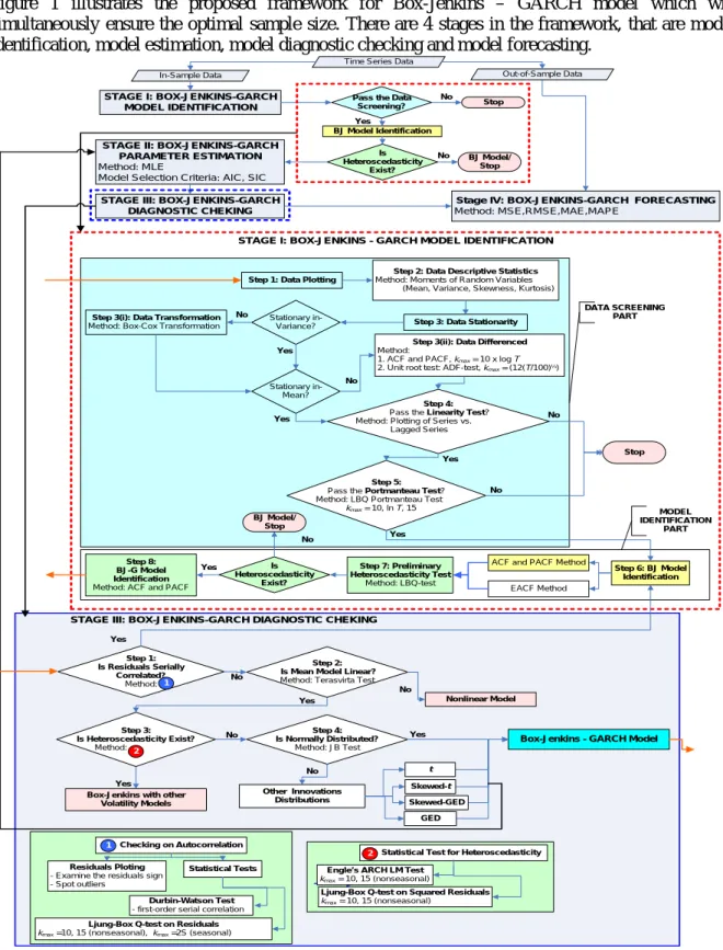
= + − = n t t t T y l y n 1 ˆ 1 MAE (5) 2.6. Proposed frameworkFigure 1 illustrates the proposed framework for Box-Jenkins – GARCH model which will simultaneously ensure the optimal sample size. There are 4 stages in the framework, that are model identification, model estimation, model diagnostic checking and model forecasting.
STAGE III: BOX-JENKINS-GARCH DIAGNOSTIC CHEKING
Step 1: Data Plotting
Step 2: Data Descriptive Statistics
Method: Moments of Random Variables (Mean, Variance, Skewness, Kurtosis)
Step 3: Data Stationarity
Stationary in-Variance?
Stationary in-Mean?
Step 4:
Pass the Linearity Test? Method: Plotting of Series vs. Lagged Series
Step 5:
Pass the Portmanteau Test? Method: LBQ Portmanteau Test kmax= 10, ln T, 15
Step 6: BJ Model Identification Stop Step 3(i): Data Transformation
Method: Box-Cox Transformation
ACF and PACF Method EACF Method DATA SCREENING PART MODEL IDENTIFICATION PART No Yes No Yes Yes No No Yes
Step 3(ii): Data Differenced
Method:
1. ACF and PACF, kmax= 10 x log T
2. Unit root test: ADF-test, kmax = (12(T/100)¼)
STAGE I: BOX-JENKINS - GARCH MODEL IDENTIFICATION Time Series Data
In-Sample Data Out-of-Sample Data STAGE I: BOX-JENKINS-GARCH
MODEL IDENTIFICATION
Pass the Data
Screening? Stop BJ Model Identification Is Heteroscedasticity Exist? No Yes
Stage IV: BOX-JENKINS-GARCH FORECASTING
Method: MSE,RMSE,MAE,MAPE
BJ Model/ Stop No
STAGE II: BOX-JENKINS-GARCH PARAMETER ESTIMATION
Method: MLE
Model Selection Criteria: AIC, SIC
STAGE III: BOX-JENKINS-GARCH DIAGNOSTIC CHEKING Is Heteroscedasticity Exist? BJ Model/ Stop No Yes
Box-Jenkins - GARCH Model
Residuals Ploting
- Examine the residuals sign - Spot outliers
Checking on Autocorrelation
Statistical Tests
Ljung-Box Q-test on Residuals kmax =10, 15 (nonseasonal), kmax =2S (seasonal)
Durbin-Watson Test
- first-order serial correlation
Statistical Test for Heteroscedasticity Engle’s ARCH LM Test
kmax = 10, 15 (nonseasonal)
Ljung-Box Q-test on Squared Residuals kmax = 10, 15 (nonseasonal) 2 1 Step 1: Is Residuals Serially Correlated? Method:1
Box-Jenkins with other Volatility Models No Yes No No Step 3: Is Heteroscedasticity Exist? Method: 2 Step 2: Is Mean Model Linear?
Method: Terasvirta Test
Step 4: Is Normally Distributed? Method: JB Test Other Innovations Distributions Skewed-GED Skewed-t t GED Yes No Nonlinear Model Yes Yes Step 7: Preliminary Heteroscedasticity Test Method: LBQ-test Step 8: BJ-G Model Identification
Method: ACF and PACF
3. Data of study
In this study, a 41-year daily world gold prices comprising of a total of 10 200 price data is used starting from 2nd January 1973 to 17th December 2013 of 5-day-per-week frequencies. Values are quoted in US dollars per ounce and the source data is obtained from www.kitco.com. However, there are some missing prices in the original series due to holiday and stock market closing day. The data series is then divided by 12 different sample sizes and each sample is tested using the proposed framework to determine the optimal sample size. Details about the data sample are summarised in table 1.
Basically, the number of data for each sample is approximately half from the previous duration, with ratio of estimate to forecast is 90:10. Based on previous study on Box-Jenkins model for nonseasonal series, Box et al. strongly suggest to use at least 50 data in model estimation [13], while Hyndman [14] suggests a minimum of 200 data and Hanke and Wichern recommend the sample size of 24 [15]. Since the original series (Sample 1) is nonseasonal and the data fit well with the Box-Jenkins model [5], the recommended sample sizes are considered in this study with slight modification.
Table 1. Data sample of study.
Sample Duration Sample Size In-Sample Data Out-of-Sample Data
1 2/1/1973 - 17/12/2013 (41-year) 10 200 2/1/1973 - 20/11/2009 (9180 data) 23/11/2009 - 17/12/2013 (1020 data) 2 24/11/1993 - 17/12/2013 (20-year) 5 000 24/11/1993 - 20/12/2011 (4500 data) 21/12/2011 - 17/12/2013 (500 data) 3 5/12/2003 - 17/12/2013 (10-year) 2 500 5/12/2003 - 18/12/2012 (2250 data) 19/12/2012-17/12/2013 (250 data) 4 22/12/2008 - 17/12/2013 (5-year) 1 250 22/12/2008 - 24/6/2013 (1125 data) 25/6/2013 - 17/12/2013 (125 data) 5 21/12/2009 - 17/12/2013 (4-year) 1 000 21/12/2009 - 29/7/2013 (900 data) 30/7/2013 - 17/12/2013 (100 data) 6 20/12/2010 - 17/12/2013 (3-year) 750 20/12/2010 - 3/9/2013 (675 data) 4/9/2013 - 17/12/2013 (75 data) 7 21/12/2011 - 17/12/2013 (2-year) 500 21/12/2011- 8/10/2013 (450 data) 9/10/2013 - 17/12/2013 (50 data) 8 19/12/2012 - 17/12/2013 (1-year) 250 19/12/2012 - 12/11/2013 (225 data) 13/11/2013 - 17/12/2013 (25 data) 9 6/3/2013 - 17/12/2013 200 6/3/2013 - 17/11/2013 (180 data) 18/11/2013 - 17/12/2013 (20 data) 10 25/6/2013 - 17/12/2013 (6-month) 125 25/6/2013 - 25/11/2013 (113 data) 2/12/2013 - 17/12/2013 (12 data) 11 2/10/2013 - 17/12/2013 55 2/10/2013 - 10/12/2013 (50 data) 11/12/2013 - 17/12/2013 (5 data) 12 6/11/2013 - 17/12/2013 30 6/11/2013 - 12/12/2013 (27 data) 13/12/2013 - 17/12/2013 (3 data)
4. Results and discussion
Based on the proposed framework for Stage I, only samples 1,2,3,4 and 7 are found to be suitable for Box-Jenkins model justified by the Portmanteau test of Ljung-Box Q-test (LBQ-test) on stationary series, st for the samples and being considered for the next analysis. Since the series for the samples
considered (samples 1,2,3,4 and 7) are nonseasonal and achieve stationarity at first differenced, therefore the Box-Jenkins of ARIMA(p,1,q) model is applied where the choice of p and q is determined using the EACF method. To justify the use of GARCH in the Box-Jenkins model, the preliminary of heteroscedasticity test using LBQ-test for squared residuals, at2 is conducted. The
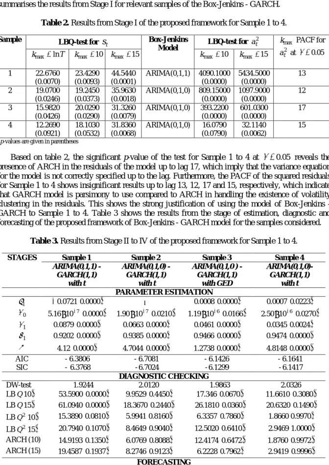
results show that sample 7 is dropped for the next stage due to no heteroscedasticity exist. Table 2 summarises the results from Stage I for relevant samples of the Box-Jenkins - GARCH.
Table 2. Results from Stage I of the proposed framework for Sample 1 to 4.
Sample LBQ-test for
t
s
Box-JenkinsModel LBQ-test for
2
t
a kmax PACF for 2
t
a at α=0.05
T
kmax =ln kmax =10 kmax =15 kmax =10 kmax =15
1 22.6760 (0.0070) 23.4290 (0.0093) 44.5440 (0.0001) ARIMA(0,1,1) 4090.1000 (0.0000) 5434.5000 (0.0000) 13 2 19.0700 (0.0246) 19.2450 (0.0373) 35.9630 (0.0018) ARIMA(0,1,0) 809.15000 (0.0000) 1097.9000 (0.0000) 12 3 15.9820 (0.0426) 20.0290 (0.0290) 31.3260 (0.0079) ARIMA(0,1,0) 393.2200 (0.0000) 601.0300 (0.0000) 17 4 12.2690 (0.0921) 18.1030 (0.0532) 31.8360 (0.0068) ARIMA(0,1,0) 16.0790 (0.0790) 32.1140 (0.0062) 15
*p-values are given in parentheses
Based on table 2, the significant p-value of the test for Sample 1 to 4 at α =0.05 reveals the presence of ARCH in the residuals of the model up to lag 17, which imply that the variance equation for the model is not correctly specified up to the lag. Furthermore, the PACF of the squared residuals for Sample 1 to 4 shows insignificant results up to lag 13, 12, 17 and 15, respectively, which indicate that GARCH model is parsimony to use compared to ARCH in handling the existence of volatility clustering in the residuals. This shows the strong justification of using the model of Box-Jenkins - GARCH to Sample 1 to 4. Table 3 shows the results from the stage of estimation, diagnostic and forecasting of the proposed framework of Box-Jenkins - GARCH model for the samples considered.
Table 3. Results from Stage II to IV of the proposed framework for Sample 1 to 4.
STAGES Sample 1 Sample 2 Sample 3 Sample 4
ARIMA(0,1,1) -GARCH(1,1) with t ARIMA(0,1,0) -GARCH(1,1) with t ARIMA(0,1,0 ) -GARCH(1,1) with GED ARIMA(0,1,0)-GARCH(1,1) with t PARAMETER ESTIMATION 1 θ −0.0721
(
0.0000)
− 0.0008(
0.0000)
0.0007(
0.0223)
0 α 5.16×10⁻⁷(
0.0000)
(
)
0210 . 0 10 90 . 1 × −7 1.19×10⁻⁶(
0.0166)
2.50×10⁻⁶(
0.0270)
1 α 0.0879(
0.0000)
0.0663(
0.0000)
0.0461(
0.0000)
0.0345(
0.0024)
1 β 0.9202(
0.0000)
0.9385(
0.0000)
0.9466(
0.0000)
0.9474(
0.0000)
ν 4.12(
0.0000)
4.7044(
0.0000)
1.2738(
0.0000)
4.8148(
0.0000)
AIC - 6.3806 - 6.7081 - 6.1426 - 6.1641 SIC - 6.3768 -6.7024 -6.1299 -6.1417 DIAGNOSTIC CHECKING DW-test 1.9244 2.0120 1.9863 2.0326 LBQ( )
10 53.5900(
0.0000)
9.9529(
0.4450)
17.346(
0.0670)
11.6610(
0.3080)
LBQ( )
15 61.0940(
0.0000)
18.3670(
0.2440)
26.1810(
0.0360)
20.6320(
0.1490)
LBQ2( )
10 15.3890(
0.0810)
5.9941(
0.8160)
6.3357(
0.7860)
1.8660(
0.9970)
LBQ2( )
15 20.7940(
0.1070)
8.4649(
0.9040)
12.5020(
0.6410)
2.9469(
1.0000)
ARCH (10) 14.9193(
0.1350)
6.0769(
0.8088)
12.4174(
0.6472)
1.8760(
0.9972)
ARCH (15) 19.4587(
0.1937)
8.2746(
0.9123)
6.2228(
0.7962)
2.9419(
0.9996)
FORECASTINGMSE RMSE MAE 4 10 4641 . 1 × − 0.0121 0.0086 4 10 5255 . 1 × − 0.0124 0.0084 4 10 9313 . 1 × − 0.0139 0.0091 4 10 9061 . 1 × − 0.0138 0.0099
*p-values are given in parentheses
Table 3 presents the results of the selection criteria (AIC and SIC) and forecasting evaluations (MSE, RMSE, MAE). In comparison of Sample 1 to 4, Sample 1 has the smallest value in the selection criteria and the forecasting evaluations. However, by applying parsimonious approach, Sample 4 is preferred since the estimation and the forecasting results are marginally decreased between the ARIMA-GARCH models that adequate to fit the data in the sample considered.
This indicates that the optimal sample size to forecast gold price using the proposed framework of Box-Jenkins and GARCH model is 1250 data of 5-year sample. The mean gold price of the 5-year sample is found to be similar to the current one that supports that the number of data in Sample 4 is sufficient enough to be used in the gold price forecasting using the hybrid model. Hence, the empirical results of model selection criteria and 1-step-ahead forecasting evaluations suggest that the latest 12.25% (5-year data) of 10200 data is sufficient enough to be employed in the Box-Jenkins and GARCH model with similar forecasting performance as by using 41-year data.
5. Conclusion
This study proposes a framework of Box-Jenkins model with GARCH which will simultaneously ensure the optimal sample size is used in analysing and forecasting higher volatile data. The empirical results of the world daily gold price indicate that the propose framework of the model is efficient and practical to be used in determining the optimal sample size while working with any univariate volatile data.
Acknowledgement
This work was supported by Universiti Malaysia Pahang via research university grant (RDU1703198).
References
[1] Yaziz S R, Azizan N A, Ahmad M H and Zakaria R 2016 Appl. Math. Sci.10 1391
[2] Yaziz S R, Azizan N A, Ahmad M H, Zakaria R, Agrawal M and Boland J 2014 Proc. 10th
IMTGT Int. Conf. Math. Stat. ITS Appl. 2014 650
[3] Ahmad M H, Ping P Y, Yaziz S R and Miswan N H 2014 Int. J. Math. Anal.8 1377 [4] Ahmad M H, Ping P Y, Yaziz S R and Miswan N H 2015 Appl. Math. Sci.9 1491
[5] Yaziz S R, Azizan N A, Ahmad M H, Zakaria R, Agrawal M and Boland J 2015 AIP Conf. Proc
1643 289
[6] Yaziz S R, Azizan N A, Zakaria R and Ahmad M H 2013 20th Int. Cong. on Modelling and
Simulation 1201
[7] Liu H and Shi J 2013 Energy Econ.37 152
[8] Tan Z, Zhang J, Wang J and Xu J 2010 Appl. Energy87 3606
[9] Zhou B, He D and Sun Z 2006 2nd Conf. on Next Generation Internet Design and Eng. 200
[10] Chen C, Hu J, Meng Q and Zhang Y 2011 IEEE Intelligent Vehicles Symp. Proc. 607 [11] Hyndman R J and Kostenko A V 2007 Foresight6 12
[12] Konishi S and Kitagawa G 2008 Biometrics64 661
[13] Box G E P, Jenkins G M and Reinsel G C 2008 Time Series Analysis, 4th Ed. (New Jersey: John Wiley & Sons, Inc.)
[14] Hyndman R J and Athanasopoulos, George 2014 Forecasting: principles and practice (OText) [15] Hanke J E and Wichern D W 2009 Business forecasting (New Jersey: Pearson/Prentice Hall)