Analysis Load Forecasting of Power System Using
Fuzzy Logic and Artificial Neural Network
Naji Ammar
1, Marizan Sulaiman
2, and Ahmad Fateh Mohamad Nor
3 1Higher Institute for Water Technology, Agelat, Libya.2,3Faculty of Electrical Engineering, Universiti Teknikal Malaysia Melaka, Hang Tuah Jaya, Durian Tunggal, Melaka, Malaysia.
Abstract— Load forecasting is a vital element in the energy management of function and execution purpose throughout the energy power system. Power systems problems are complicated to solve because power systems are huge complex graphically widely distributed and are influenced by many unexpected events. This paper presents the analysis of load forecasting using fuzzy logic (FL), artificial neural network (ANN) and ANFIS. These techniques are utilized for both short term and long-term load forecasting. ANN and ANFIS are used to improve the results obtained through the FL. It also studied the effects of humidity, temperature and previous load on Load Forecasting. The simulation is done by the Simulink environment of MATLAB software.
Index Terms— ANFIS; Artificial Neural Networks (ANN); Fuzzy Logic (FL); Load Forecasting.
I. INTRODUCTION
Generally speaking, load forecasting is a piece of technology used by utility corporations to determine the equilibrium point between demand and supply of electricity, and the beneficiaries include banks, companies, businesses, industries, governments, private residences, and many others. The importance of this technology is very vast as it serves as a function of pricing and evaluation in the energy industry and it also provides the companies and stakeholders with the accurate forecast in the operation and management of the industry and decision making [1,2]. It is the white blood cell of the energy companies by ensuring security, reliability, and cost-effectiveness under which a deregulation spurs aggressive competitiveness and determination of rates versus investment analysis. To forecast a load, there are many factors by which the companies must take into account if they are to arrive at a near-accurate estimation, even though in such handling of information estimations are not always 100 % perfect [3]. The companies take into account the time, the weather, the classes of customers, the temperature range, humidity, and population and other relevant information. There are three ways of conducting this analysis: the short-term, medium-term, and the long-term load forecast. In brief, the short term is aligned to a short period, and it contains the forecast for one hour and a week. The medium term extends from one week to the maximum of a year ahead and in long-term forecast, the time frame starts from one year too many[4,5]. Certainly, many methodologies dominate the whole process of load forecasting ranging from regression method, exponential smoothing, stochastic process, ARMA, to data mining; et cetera. However, the most recent and shared
methodology in the present has been subsumed into a term called artificial intelligence (a combination of artificial neural networks (ANN) and fuzzy logic). Although the artificial neural network method is reasonable in some sense, it has been the least preferred compared to the fuzzy logic method which is garnered around tremendous flexibility. Thus, this paper will review the technology of load forecasting around the context of a fuzzy logic approach, and artificial neural network method combined [6,7].
II. TYPES OF LOAD FORECASTING
There are three different main types of load forecasting, and they are [8, 9, 10, 11]:
A. Short -Term Load Forecast (STLF). B. Medium -Term Load Forecast (MTLF). C. Long -Term Load Forecast (LTLF).
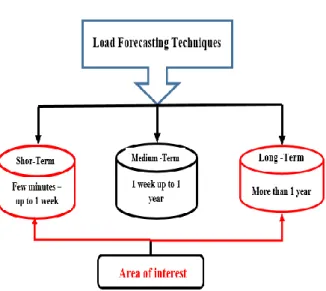
Short-term load forecasting (STLF) is essentially is a predicting load system with a leading time of one hour to a week. Medium -term load forecast (MTLF) is essentially is a load predicting system with a leading time of one week up to 1 year. Long -term load forecast (LTLF) is essentially is a load predicting system with a leading time more than one year. The main objective of short -term load forecast (STLF) is economic load dispatch, load scheduling, reliability and system security assessment. STLF has high forecasting accuracy, and speed response are both significant to analyze the load characteristics, this type of prediction is concerned about control on energy transaction, security, fuel consumption, maintenance, unit scheduling and others. Similarly, there are varieties of functions in this regard such as regulation of smooth load flow, overloading, and blackouts. For MTLF several objectives should be considered such as the development of power system infrastructure, tariff and purchase agreements, peak load, etc. MTLF has medium forecasting accuracy, and the common response is both significant to analyze the load characteristics. LTLF the last one type of load forecasting. The main objective of LTLF must take into accounts such as future expansions, improved distribution facilities, economic planning, infrastructural, technological developments and Utilities usually count the population LTLF has low forecasting accuracy, and slow response is both significant to analyze the load characteristics. Some effects must take into account concerning accuracy in types of load forecasting such as inappropriate data selection and Pauper data analysis drive to a decreased accuracy.
Many factors are influencing on types of load forecasting some of them weather variables such as temperature, humidity, wind speed, rainfall and wind chill and another factor load consumption variables like hourly load, weekly load, and peak load. The common estimation model is, however, classified into two-fold parametric and intelligence method. The parametric model commands trend analysis end –use and econometric modeling as in the case of MTLF. However, the problems of uncertainty, fluctuation, and possible obsolescence or absence of data matches both the MTLF and LTLF. Figure 1 shows the basic load forecasting techniques.
Figure 1: Basic load forecasting techniques III. METHODS OF LOAD FORECASTING A. Fuzzy Logical System (FLS)
The origin of the “fuzzy logic” emanates from a theory called fuzzy set created by Dr. L.A. Zadeh in the middle of 1960s. The fuzzy logic used a mathematical model which resonates human mental syntax on IF-THEN basis by mirroring a nonlinear relationship between weather parameters and how they affect the daily electric power load. Fuzzification is the process of aligning fuzzy sets with membership functions which carry crisp numerical values. These membership functions have different model classifications; namely, trapezoidal, Gaussian, triangular, etc. However, for this review paper, the triangular model is used because of its flexibility in data handling. The membership function is the attachment of member value to every input space (normally between 0 up to 1. The next step is about the fuzzy inference system, and it means that data is taken on a limited basis (IF-THEN) and import to the inference system which analyzes the data to produce the forecasted load output (KW) as shown in Figure 2 [12].
Figure 2: Block diagram of fuzzy model
B. Artificial Neural Networks (ANN)
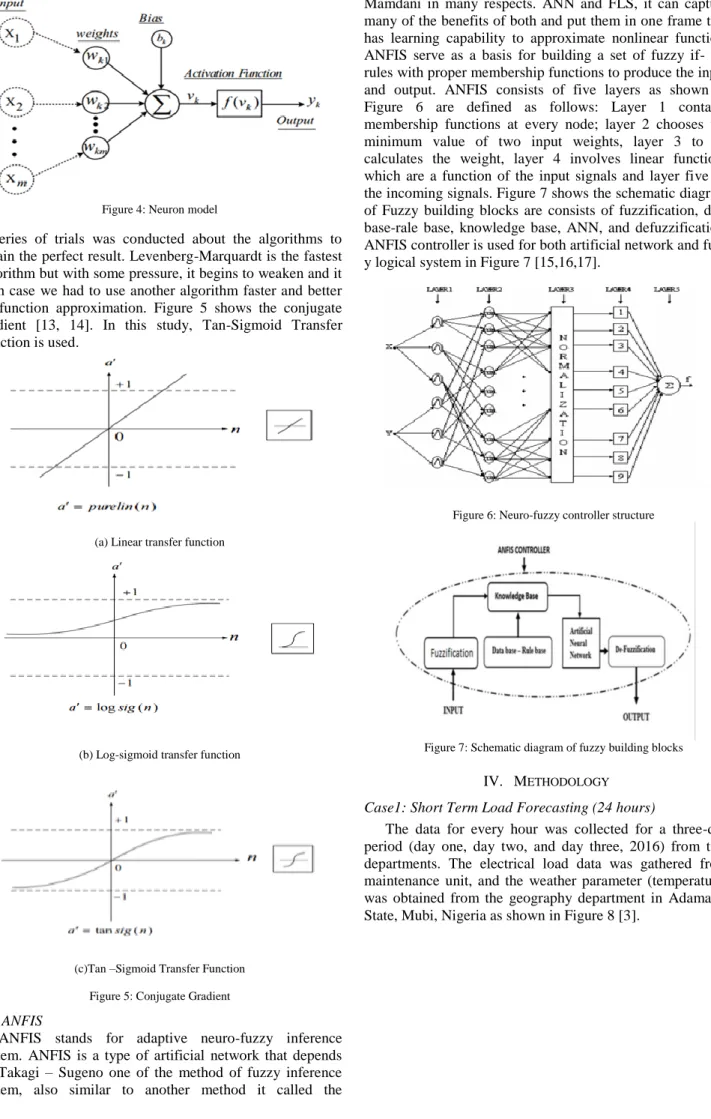
This is a unique modeling tool that handles complex data inputs and outputs, and historically this was designed to act like the human ‘intelligence.' The similarities between the ANN and the human brain: Knowledge comes from learning; and that the knowledge is stored in synaptic weights and this is the beginning of the brain related product. The ANN is a remarkable advancement in the computational industry. Neurons as the core element, pick input, process it, and conduct all the operations and extract the final output. The main components of the inputs are the temperature, humidity, time, the wind, the previous day load, hour of the day. The ANN is being issued for load forecasting yet a significant amount of error is made due to distortion in the fluctuations in load and temperatures. The neural networks are easily compatible with sensory data dealing. The neural networks is a mathematical model with it operates and looks similarly like the brain. It contains unit ‘cells’ or ‘nodes’ which netted together. When the inputs (cells) are triggered, the signals go through the network through a note-to-note and exit the network through another particular node. These computational nodes are not linear. The neural network models were grouped into network topology, attributes of node, training or rules of learning as seen in Figure 3.
Figure 3: Block diagram for neural network model
Back propagation is slow in the case of real problems, but high-performance algorithms may seem faster than the back propagation. Moreover, these high-performance algorithms have two main divisions. The first being heuristic technique (variable rate and resilient back propagation. Another division is numerical optimization technique (conjugate gradient, quasi-newton, Levenberg-Marquardt). This neuron model was demonstrated in Figure 4.
𝑣𝑘= ∑ 𝑗𝑤𝑘𝑗+ 𝑏𝑘 𝑚
𝑗=1
(1)
Figure 4: Neuron model
Series of trials was conducted about the algorithms to obtain the perfect result. Levenberg-Marquardt is the fastest algorithm but with some pressure, it begins to weaken and it such case we had to use another algorithm faster and better on function approximation. Figure 5 shows the conjugate gradient [13, 14]. In this study, Tan-Sigmoid Transfer Function is used.
(a) Linear transfer function
(b) Log-sigmoid transfer function
(c)Tan –Sigmoid Transfer Function Figure 5: Conjugate Gradient C. ANFIS
ANFIS stands for adaptive neuro-fuzzy inference system. ANFIS is a type of artificial network that depends on Takagi – Sugeno one of the method of fuzzy inference system, also similar to another method it called the
Mamdani in many respects. ANN and FLS, it can capture many of the benefits of both and put them in one frame that has learning capability to approximate nonlinear function. ANFIS serve as a basis for building a set of fuzzy if- the rules with proper membership functions to produce the input and output. ANFIS consists of five layers as shown in Figure 6 are defined as follows: Layer 1 contains membership functions at every node; layer 2 chooses the minimum value of two input weights, layer 3 to do calculates the weight, layer 4 involves linear functions which are a function of the input signals and layer five all the incoming signals. Figure 7 shows the schematic diagram of Fuzzy building blocks are consists of fuzzification, data base-rale base, knowledge base, ANN, and defuzzification. ANFIS controller is used for both artificial network and fuzz y logical system in Figure 7 [15,16,17].
Figure 6: Neuro-fuzzy controller structure
Figure 7: Schematic diagram of fuzzy building blocks IV. METHODOLOGY
Case1: Short Term Load Forecasting (24 hours)
The data for every hour was collected for a three-day period (day one, day two, and day three, 2016) from two departments. The electrical load data was gathered from maintenance unit, and the weather parameter (temperature) was obtained from the geography department in Adamawa State, Mubi, Nigeria as shown in Figure 8 [3].
Figure 8: Block diagram representation
Temperature and time are fused into the fuzzy logical system; then an output is obtained then inserted into the neural networks with the previous data (24-hour) load and target. The output (load predictive) of the network is then compared to the desired production and the weight adjustment through the network to obtain the right or appropriate mapping.
Fuzzification
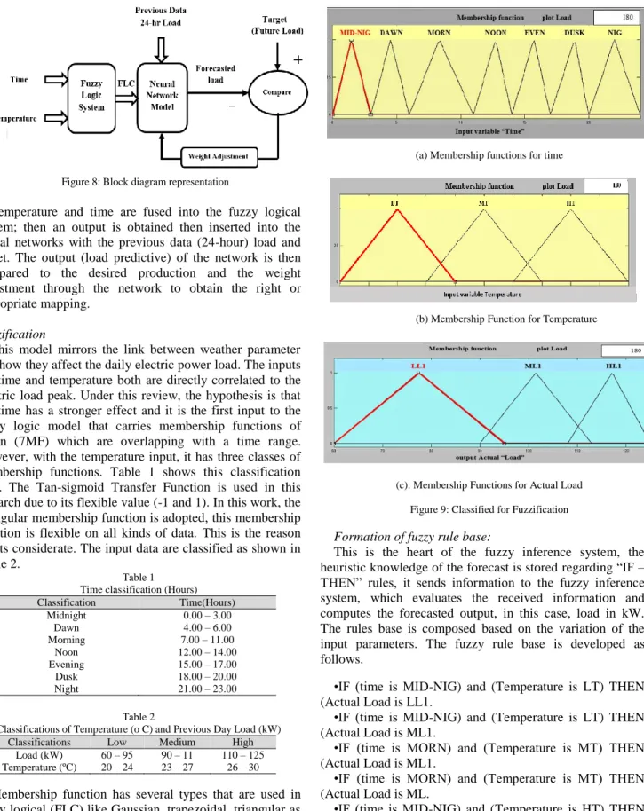
This model mirrors the link between weather parameter and how they affect the daily electric power load. The inputs are time and temperature both are directly correlated to the electric load peak. Under this review, the hypothesis is that the time has a stronger effect and it is the first input to the fuzzy logic model that carries membership functions of seven (7MF) which are overlapping with a time range. However, with the temperature input, it has three classes of membership functions. Table 1 shows this classification [16]. The Tan-sigmoid Transfer Function is used in this research due to its flexible value (-1 and 1). In this work, the triangular membership function is adopted, this membership function is flexible on all kinds of data. This is the reason for its considerate. The input data are classified as shown in Table 2.
Table 1 Time classification (Hours) Classification Time(Hours) Midnight 0.00 – 3.00 Dawn 4.00 – 6.00 Morning 7.00 – 11.00 Noon 12.00 – 14.00 Evening 15.00 – 17.00 Dusk 18.00 – 20.00 Night 21.00 – 23.00 Table 2
Classifications of Temperature (o C) and Previous Day Load (kW) Classifications Low Medium High
Load (kW) 60 – 95 90 – 11 110 – 125 Temperature (ºC) 20 – 24 23 – 27 26 – 30 Membership function has several types that are used in fuzzy logical (FLC) like Gaussian, trapezoidal, triangular as shown in Figure 9 [16]. The use triangular for this work and the value of mapping is usually between (0, 1).
(a) Membership functions for time
(b) Membership Function for Temperature
(c): Membership Functions for Actual Load Figure 9: Classified for Fuzzification Formation of fuzzy rule base:
This is the heart of the fuzzy inference system, the heuristic knowledge of the forecast is stored regarding “IF – THEN” rules, it sends information to the fuzzy inference system, which evaluates the received information and computes the forecasted output, in this case, load in kW. The rules base is composed based on the variation of the input parameters. The fuzzy rule base is developed as follows.
•IF (time is MID-NIG) and (Temperature is LT) THEN (Actual Load is LL1.
•IF (time is MID-NIG) and (Temperature is LT) THEN (Actual Load is ML1.
•IF (time is MORN) and (Temperature is MT) THEN (Actual Load is ML1.
•IF (time is MORN) and (Temperature is MT) THEN (Actual Load is ML.
•IF (time is MID-NIG) and (Temperature is HT) THEN (Actual Load is HL1.
•IF (time is NOON) and (Temperature is HT) THEN (Actual Load is HL1.
•IF (time is EVEN) and (Temperature is MT) THEN (Actual Load is HL1.
•IF (time is DUSK) and (Temperature is LT) THEN (Actual Load is HL1.
•IF (time is DUSK) and (Temperature is LT) THEN (Actual Load is ML1.
•IF (time is NIG) and (Temperature is LT) THEN (Actual Load is LL.
The building of Fuzzy Logic Simulation Model between Time and Temperature (short-term for one week).
The fuzzy model is developed, where the two inputs are multiplexed and sent to the fuzzy logic controller with rule viewer, which will process the aggregate information and produces a crisp output value as shown on the display of Figure 10. For example, a sample input of temperature 180𝐶 and the time at 4.00 am were simulated and the forecasted load obtained is 92.5kW. This can also be seen on rule viewer in Figure 11. The rule viewer below shows the plots of antecedent (time and temperature) consequent (forecasted load).
Figure 10: Simulation Diagram of Simulink
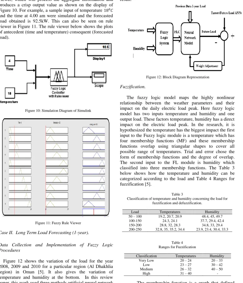
Figure 11: Fuzzy Rule Viewer Case II. Long Term Load Forecasting (1-year).
Data Collection and Implementation of Fuzzy Logic Procedures
Figure 12 shows the variation of the load for the year 2008, 2009 and 2010 for a particular region (Al Dhakhlia region) in Oman [5]. It also gives the variation of temperature and humidity at the bottom. In this review paper, this work used three methods artificial neural network (ANN), Fuzzy Logic (FLC) and ANFIS. Here two parameters are considered one is the temperature, and the other is the humidity. In this research, the humidity and the temperature data is fed to the fuzzy logic system, and the output combines with previous data (1-year) load and target (future load ANN) load proportional to these two
parameters. Moreover, comparing the actual load (target) with the fore casting load and check the effect of weather parameter (temperature and humidity) on electric load. Finally, three parameter data (T, H, P) are fed to the ANFIS and output is a target (future load ANN) to obtained good result.
Figure 12: Block Diagram Representation Fuzzification.
The fuzzy logic model maps the highly nonlinear relationship between the weather parameters and their impact on the daily electric load peak. Here fuzzy logic model has two inputs temperature and humidity and one output load. These factors temperature, humidity has a direct impact on the electric load peak. In the research, it is hypothesized the temperature has the biggest impact the first input to the Fuzzy logic module is a temperature which has four membership functions (MF) and these membership functions overlap using triangular shapes to cover all possible range of temperatures. Trial and error chose the form of membership functions and the degree of overlap. The second input to the FL module is humidity which classified into three membership functions. The Table 3 below shows how the temperature and humidity can be categorized according to the load and Table 4 Ranges for fuzzification [5].
Table 3
Classification of temperature and humidity concerning the load for fuzzification and defuzzification.
Load Temperatures Humidity
50 – 100 19.2, 20.7, 20.9 48.4, 45, 49.7 100-150 24.3, 24.1 37.7, 29.4, 42.4 150-200 28.8, 32, 28.3 34.8, 33, 29.4 200-250 32.8, 35, 35.2, 34.4 23.9, 23.4, 30.4, 33.3
Table 4 Ranges for Fuzzification
Classification Temperatures Humidity
Very Low 20 – 24 20 – 33
Low 23 – 27 30 – 42
Medium 26 – 32 40 – 50
High 31 – 40
-The membership function is a graph that defined how each point in the input space is mapped to its member value. This is usually between 0 and 1. Various classification of load the corresponding temperature and humidity are taken. Then the ranges of Fuzzification are obtained as shown in the second part of the table4. The Figure 13 [5] illustrate how the inputs are classified for
Fuzzification. It is observed that the temperatures are classified with the ranges (20-24), (23-27), (26-32), (31-40) as Very Low, Low, Medium and high respectively. The humidity is classified as (20-33), (30-42), (40-50) as Low, Medium and High respectively. The outputs are classified as (50-110), (100-160), (150-200), and (200-250) as Very Low, Low, Medium and High Loads respectively.
(a) Membership function for temperature
(b) . Membership function for relative humidity
(c). Membership function for load Figure 13: Classified for Fuzzification Formation of Fuzzy Rule Base:
The rules base is composed based on the variation of the input parameters.
1-If (temperature is medium Temp) and (Humidity is low Humidity) then (then is medium load).
2- If (temperature is high Temp) and (Humidity is low Humidity) then (Load is High Load).
3- If (temperature is Very Low Temp) and (Humidity is Medium humidity) then (Load is a low load.
4- If (temperature is low temp) and (Humidity is Medium) then (Load is a low load.
5- If (temperature is Medium temp) and Humidity is Medium Humidity then (load is Medium load).
6- If (temperature is High Temp) and (humidity is Medium humidity then (Load is High Load).
7- If (temperature is Very Low Temp) and Humidity is High Humidity) then (Load is a Very Low load.
Data Collection and Implementation of ANN for Short Term Load Forecasting (24hour).
The Collection data can be divided into two types which are actual load and the hourly weather parameters such as
time and temperature; Both were taken from the geography department in Adamawa State, Mubi, Nigeria for one week as shown in Figure 8. Moreover, it covers 168 hours from first January 2016 to seven January 2016.
Implementation of ANN using MATLAB
Using the historical data as seen in table 5 and saved in an Excel spreadsheet. This data set spans of one week which are equal 168 hours, the neural network consisting of the two-layer feedforward network with hidden sigmoid neurons and linear output neurons and also used for training with Leven Berg–Marquardt backpropagation algorithm as seen in Figure 14.
Figure 14: ANN open tool in MATLAB
The next step we choose the data which is divided into two Categories one of them is the input of weather variables such as temperature, time and previous data 24 hours load on load forecasting and other is a target for output as shown in Figure 15. Training was set to 70%, validation was 15%, and Testing was 15% number of hidden neurons ten if the error is high then to minimize the error retrain is done then we can obtain plots of the implement, Train state, Fit and Regression as shown in Figure 16.
Figure 16: Training, validation, and testing setting
Figure 17 shows the results of the ANN. Only seven iterations were needed by this ANN to complete the task. This ANN only consumed a small amount of time which is 0.001 seconds. The performance of the ANN is very good with a mean squared error value of 1.13e-22.
Figure 17: Training state, fit, and regression
Figure 18 Shows the ANN performance plot. The total number of epoch produced is 9. It also can be seen that the best validation performance is 1337.3492 at epoch 9.
Figure 18: ANN performance plot Implementation of ANFIS using MATLAB
The ANFIS modeling standard was adopted to effectively melody the membership function to decrease the
output error and maximize performance indicator. ANFIS Editor Display made up four types are. Load data, General is, Train Fis and Test FIs, the load data is used for training, testing, and checking. Next stage is to click generate FIS and select any type such as trim and trapmf; the finally is select linear as shown in Figure 19.
Figure 19: ANFIS editor
Generating the Fuzzy Rules and select the Membership Function.
The first steps after successfully downloading the training data, the rules are produced by the grid division method. We have five (5) inputs with four (4) membership function; the rule group contains, 45 i.e. 1024 rules. Network
partitioning is an approach for initializing the framework in a fuzzy inference system. In this way, it produces rules by recount all possible installations of the membership function of all inputs as shown in Figure 20.
Figure 20: The dialog box of the rule viewer
The building of Fuzzy Logic Simulation Model between Humidity and Temperature (Long-term for five years).
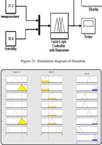
The Figure 21 shows the Simulink used to simulate. The first input to the FL is temperature, and the other is the humidity both send to the fuzzy logic controller with rule viewer and output value as shown on display.
It is observed from the simulation that for a temperature of 35.20 C and 30.4% relative humidity the load is 224.5MW. The Figure 22 demonstrates how the fuzzy system in MATLAB toolbox which works for the sample inputs. For example, it is seen that the High temperature and low humidity gives an output of High load, similarly for low temperature and high humidity the output is Very Low
Load. This can be cross-checked with the actual load in the Table 5 which shows that the load is 225 MW.
Figure 21: Simulation diagram of Simulink
Figure 22: Fuzzy rule viewer ANFIS
The ANFIS modeling standard was adopted to effectively melody the membership function to decrease the output error and maximize Performance indicator. The ANFIS structure gained by the mentioned parameters selection is shown in Figure 23. Figure 24 illustrates the relationship between the target and outputs are closeness. R value of one (R=1) indicates a perfect. From the regression plot R=0.9045 for training, R=0.49745 for validation, R=0.0017539 for testing and R=0.5613 for all.
Figure 24: Regression plot V. RESULTS AND DISCUSSION Case I. Short-Term Load forecasting (24-hour).
This work, an Artificial Neural Network
Backpropagation (ANN
-
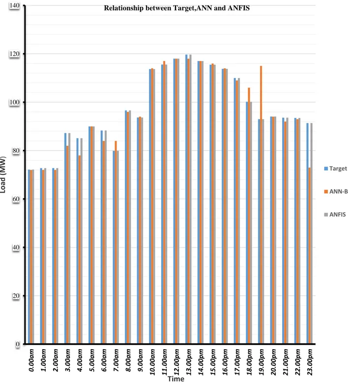
BP) which is made up of three layers (input layer, a hidden layer, and output layer) was established. The Sigmoid Transfer Function is used for the Transfer Function between the input and the hidden layer, and the logsig Function for that between the hidden layer and the output layer. The input is number neurons, and the hidden layers must be optimized. Through simulation studies on the short-term load forecasting (24-hours) as shown in Table 5, it is observed that from midnight up to 6.00 am the load is low, and load increases at 8.00 am. The relationship between load and time of the day is obtained in Table 5. It can also be seen from Table 5 that Absolute Percentage Error values vary from 1.03% to 24.77%. The forecasting is done for 24 hours daily. The biggest error from ANN-BP on 2nd January 2016 was at 0.00 am, 24.77% and the load reached its peak at 13.00 PM; this refers to the rise in temperature at that time. The Table 5 below illustrates the results obtained from data management and analysis were performed using MATLAB in the order obtained the relationship between forecasted load and Actual load. Through the results show it is very close. Finally, it is observed from Figure 16 that ANFIS has higher accuracy, faster response and more suitable for the application compare to ANN-BP and FL. It also helps in finding the number of rules from fuzzyTable 5
Hourly Load Forecast of 2nd January 2016
5- Input data short –term ANN ANFIS
Time Temperature (0C) Previous 24-hr (kW) Forecast load (kW FLC Target Output % Error Output % Error 0.00 am 19 69.25 90 90 72.13 72 24.77 72.13 0 1.00 am 20 70.50 85 90 72.75 72 23.7 72.75 0 2.00 am 19 69.50 85 85 72.75 72 16.8 72.75 0 3.00 am 18 82.50 90 86 87.25 82 1.4 87.25 0 4.00 am 18 77.75 90 92.5 85.13 78 5.7 85.13 0 5.00 am 19 87.5 90 92.5 90 90 2.8 90 0 6.00 am 19 84 90 92.5 88.3 84 4.75 88.3 0 7.00 am 20.5 84.8 98.2 92.5 79.9 84 15.7 79.9 0 8.00 am 23.5 95 98.2 102 96.6 96 5.6 96.6 0 9.00 am 26 95 96 101.5 93.7 94 8.3 93.7 0 10.00 am 27 112.5 122 92.5 113.7 114 18.6 113.7 0 11.00 am 27.5 116 113 92.5 115.6 117 19.98 115.6 0 12.00 pm 27 121 112 116.6 118 118 1.18 118 0 13.00 pm 27 124.5 113 116.6 119.7 118 2.6 119.7 0 14.00 pm 26.5 119 112 92.5 117 117 20.9 117 0 15.00 pm 25.5 116 112 116.7 115.5 116 1.03 115.5 0 16.00 pm 24.5 112.5 112 116.6 113.8 114 2.46 113.8 0 17.00 pm 24 105 100 92.5 110 109 15.9 110 0 18.00 pm 24 97.5 101 92.5 100.2 106 7.68 100.2 0 19.00 pm 23 94 93 107.7 93 115 15.8 93 0 20.00 pm 22 90 90 92.5 94.1 94 1.7 94.1 0 21.00 pm 22 89 90 92.5 93.6 92 1.16 93.6 0 22.00 pm 22 89 90 77.5 93.5 93 17.11 93.5 0 23.00 pm 20.5 85 90 77.5 91.4 73 15.2 91.4 0 Average ANN 10.45 ANFIS 0
Figure 25: Output ANN – BP
Case II. Long Term Load Forecasting (1- year).
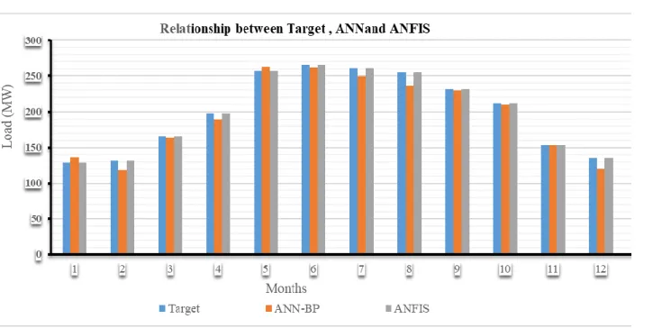
Table 6 shows the relationship between the temperatures, relative humidity with the future load. It can be seen that the increase in temperature values will lead to the increase of load values. On the contrary, the increase in relative humidity will result in the decrease of load values. Also, it can also be seen that the combination of minimum
temperature with maximum humidity will obtain minimum load value. Table 6 also conveys that the average error of ANN-BP and ANFIS are 7.66% and 0.00006%, respectively. Figure 26 depicted the comparison between the target, ANN-BP, and ANFIS.
0 20 40 60 80 100 120 140 0.0 0am 1.0 0am 2.0 0am 3.0 0am 4.0 0am 5.0 0am 6.0 0am 7.0 0am 8. 0 0am 9.0 0am 10. 00am 11. 00am 12. 00pm 13. 00pm 14. 00pm 15. 00pm 16. 00pm 17. 00pm 18 .00 pm 19. 00pm 20. 00pm 21. 00pm 22. 00pm 23. 00pm
Lo
ad
(
M
W
)Time
Relationship between Target,ANN and ANFIS
Target
ANN-BP ANFIS
Table 6
Temperature -Relative Humidity- Previous 24-h
Figure 26: Output ANN – BP
VI. CONCLUSION
In this research, a methodology for load forecasting using fuzzy logic, artificial neural network, and ANFIS approach is presented. This research has successfully simulated load forecasting with the use of FL, ANN-BP, and ANFIS. The results have shown that both ANN-BP and ANFIS can predict forecasting load values. However, ANFIS gives much more accurate results compared to ANN-BP.
Furthermore, ANFIS is capable of producing its number of rules and membership functions.
ACKNOWLEDGMENT
The authors are grateful to the Universiti Teknikal Malaysia Melaka for providing the necessary platform for this research to Center for Robotics and Industrial Automation (CeRIA).
5- Input data short –term ANN ANFIS
Month Tempera -true Relative Humidity Predicted Load (KW) Previous 24-hr (KW) FLC (KW Target
Output %Error Output %Error
1 19.2 48 84.35 78 150 128.85 129 8.14 128.85 0 2 20.7 45 86.8 75 79.97 131.3 128.86 15.75 131.3 0 3 24.3 37.7 120.65 123 129.6 165.15 134.99 1.91 165.15 0.0001 4 28.8 29.4 152.8 172 174.8 197.3 128.85 11.16 197.3 0.0001 5 32.8 23.9 213.15 223 224.6 257.65 128.85 4.41 257.65 0.0002 6 35.0 23.4 221.775 223 224.6 266.27 128.85 0.549 266.27 0 7 35.2 30.4 216.7 224 224.5 261.2 128.85 3.25 261.2 0.0003 8 34.4 33.1 210.7 221 224.6 255.2 128.85 4.66 255.2 0 9 32.0 33 186.4 220 224.5 230.9 128.85 15.27 230.9 0 10 28.3 34.8 167.8 173 174.7 212.3 128.85 3 212.3 0 11 24.1 42.4 109.15 122 150 153.65 151.58 10.33 153.65 0 12 20.9 49.7 90.8 80 80 135.3 128.86 13.5 135.3 0
REFERENCES
[1] P. Gohil and M. Gupta, “Short Term Load Forecasting Using Fuzzy Logic,” Int. J. Eng. Dev. Res., vol. 10, no. 3, pp. 127–130, 2014. [2] H. A. Abdulqader, “Load Forecasting for Power System Planning and Operation Using Artificial Neural Network At Al Batinah Region Oman,” J. Eng. Sci. Technol., vol. 7, no. 4, pp. 498–504, 2012. [3] A. Danladi, M. I. Puwu, Y. Michael, and B. M. Garkida, “Use of Fuzzy Logic To Investigate Weather Parameter Impact on Electrical Load Based on Short Term Forecasting,” Niger. J. Technol., vol. 35, no. 3, pp. 562–567, 2016.
[4] P. GL, K. Sambasivarao, P. Kirsali, and V. Singh, “Short Term Load Forecasting for Uttarakhand using Neural Network and Time Series models,” IEEE Int. Conf., vol. On the page, no. S, pp. 1–6, 2014. [5] S. R and H. A. Al Abdulqader, “Load forecasting for Power System Planning Using Fuzzy-Neural Network,” in Proceedings of the World Congress on Engineering and Computer Science, 2012, vol. I. [6] W. E. I. Sun, “Application of Neural Network Model Based on Combination of Fuzzy Classification and Input Selection in Short Term Load Forecasting,” Mach. Learn., no. August, pp. 3153–3156, 2006. [7] S. M. D. E. Rocco, A. R. Aoki, M. V. Lamar, C. E. P. Brazil, and C. E. P. Brazil, “Load Forecasting Using Artificial Neural Networks and Support Vector Regression,” pp. 36–41, 2007.
[8] S. R. Khuntia, J. L. Rueda, and M. A. M. M. van der Meijden, “Forecasting a load of electrical power systems in mid- and long-term horizons: a review,” IET Gener. Transm. Distrib., vol. 10, no. 16, pp. 3971–3977, 2016.
[9] L. Ghods and M. Kalantar, “Different methods of long-term electric load demand forecasting; a comprehensive review,” Iran. J. Electr. Electron. Eng., vol. 7, no. 4, pp. 249–259, 2011.
[10] Z. M. Shamseldin, “Short Term Electrical Load Forecasting Using Fuzzy Logic,” no. November 2015.
[11] E. Badar and U. Islam, “Comparison of Conventional and Modern Load Forecasting Techniques Based on Artificial Intelligence and Expert Systems,” Int. J. Comput. Sci. Issues, vol. 8, no. 5, pp. 504– 513, 2011.
[12] M. Mustapha, M. W. Mustafa, S. N. Khalid, I. Abubakar, and H. Shareef, “Classification of electricity load forecasting based on the factors influencing the load consumption and methods used: An-overview,” 2015 IEEE Conf. Energy Conversion, CENCON 2015, pp. 442–447, 2016.
[13] S. Amakali, “Development of models for short-term load forecasting using artificial neural networks,” 2008.
[14] M. Hayati and Y. Shirvany, “Artificial neural network approach for short term load forecasting for Illam region,” World Acad. Sci. Eng. Technol., vol. 1, no. 4, pp. 121–125, 2007.
[15] J. Sruthi and R. L. H. Catherine, “A Review on Electrical Load Forecasting in Energy Management,” Int. J. Innovative Sci. Eng. Technol., vol. 2, no. 3, pp. 670–676, 2015.
[16] K. Bagherifard, O. Ibrahim, S. Izman, N. Janahmadi, and M. Barisamy, “Application of Anfis System in Prediction of Machining Parameters,” J. Theor. Appl. Inf. Technol., vol. 33, no. 1, 2011.
[17] L. Rajaji, C. Kumar, and M. Vasudevan, “Fuzzy and Anfis Based Soft Starter Fed Induction Motor Drive for High-Performance Applications,” ARPN J. Eng. Appl. Sci., vol. 3, no. 4, pp. 12–24, 2008.