Data envelopment analysis and
data mining to e
ffi
ciency
estimation and evaluation
Abdel Latef M. Anouze
Department of Management and Marketing, Qatar University, Doha, Qatar, and
Imad Bou-Hamad
Suliman S. Olayan School of Business, American University of Beirut, Beirut, Lebanon
Abstract
Purpose–This paper aims to assess the application of seven statistical and data mining techniques to second-stage data envelopment analysis (DEA) for bank performance.
Design/methodology/approach–Different statistical and data mining techniques are used to second-stage DEA for bank performance as a part of an attempt to produce a powerful model for bank performance with effective predictive ability. The projected data mining tools are classification and regression trees (CART), conditional inference trees (CIT), random forest based on CART and CIT, bagging, artificial neural networks and their statistical counterpart, logistic regression.
Findings–The results showed that random forests and bagging outperform other methods in terms of predictive power.
Originality/value– This is thefirst study to assess the impact of environmental factors on banking performance in Middle East and North Africa countries.
Keywords Bank performance, Data envelopment analysis, MENA countries, Data mining tools Paper typeResearch paper
1. Introduction
Sustainability is one of the concepts which has been associated with bank performance; therefore, assessing and predicting bank performance have become vital for managers when examining the suitability of their managerial decisions. Additionally, studying bank performance greatly facilitates measuring the success of decisions made by a bank as compared to those of its counterpart during the same period. Furthermore, it allows one to learn how to make betterfinancial decisions that allocate financial resources in a more efficient manner. There is substantial body of published academic research that discusses different methods of evaluating bank performance;Berger and Humphrey (1997)grouped them into two main approaches, namely, parametric and nonparametric. The most popular parametric method is known as the stochastic frontier approach (SFA), whereas the most
© Abdel Latef M. Anouze and Imad Bou-Hamad. Published by Emerald Publishing Limited. This article is published under the Creative Commons Attribution (CC BY 4.0) licence. Anyone may reproduce, distribute, translate and create derivative works of this article (for both commercial and non-commercial purposes), subject to full attribution to the original publication and authors. The full terms of this licence may be seen at http://creativecommons.org/licences/by/4.0/legalcode
Data
envelopment
analysis
169
Received 13 November 2017 Revised 15 January 2018 25 May 2018 8 September 2018 Accepted 10 November 2018International Journal of Islamic and Middle Eastern Finance and Management Vol. 12 No. 2, 2019
pp. 169-190
Emerald Publishing Limited 1753-8394 DOI10.1108/IMEFM-11-2017-0302
The current issue and full text archive of this journal is available on Emerald Insight at: www.emeraldinsight.com/1753-8394.htm
popular nonparametric method is data envelopment analysis (DEA). Although using these methods could help researchers determine performance level, they are not sufficient to explain inefficiency or predict performance. Therefore, several studies, like that ofFethi and Pasiouras (2010), proposed a combination of measuring and explaining bank performance using DEA or SFA in thefirst stage to measure performance and regression models as a second stage to explain it.Casu and Molyneux (2003);Ariff and Can (2008)andSanet al. (2011)used Tobit regression in particular to explain bank performance. Other researchers used different regression models to explain bank performance;Anouze (2010);Emrouznejad and Anouze (2010)andBou-Hamadet al.(2017)used boosted generalized linear model, and
Seolet al.(2007)used decision trees, whereasAzadehet al.(2011)used the artificial neural
networks (ANNs). On the other hand,Sun and Li (2008) andWu and Hsu (2019) used decision tree techniques to introduce a multiple criteria decision-making method to determine suitable warning mechanisms of corporate financial failure or distress. Meanwhile,Laiet al.(2011)used DEA to develop an intellectual benchmarking knowledge-based system for benchmarking, performance evaluation and process improvement.
However, no comparison of methods used in second DEA stage has been made, and most of these studies aimed only to explain the factors affecting efficiency rather than predicting future efficiency of banks. Predicting bank performance is extremely important: bad performance may lead to bankruptcy, which negatively influences the economy of a country. Thus, conceiving a powerful predictive model for bank performance would be useful in avoiding or at least limiting such consequences. Therefore, this study proposes a comprehensive performance evaluation framework based on managerial,financial and macroeconomic indicators to predict bank performance. More specifically, seven predictive techniques, namely, classification and regression trees (CART), conditional inference trees (CIT), random forest based on CART (RF-CART), random forest based on CIT (RF-CIT), bagging, ANNs and logistic regression (LR) are assessed when applied to second-stage DEA. This framework is applied to a data set of 151 banks from Middle East and North Africa (MENA) countries observed over a period of three years (2008-2010); hence, the data set contains 453 observations with 15 environmental variables (predictors). For predictive comparison among the used data mining methods, we used the overall accuracy, sensitivity, specificity and the areas under the ROC curve (AUC).
The following sections are organized as follows: Section 2 reviews the related literature and Section 3 describes DEA and data mining methods used. Section 4 describes the MENA banks data set. The experimental set up and model performance measures used in our comparison are described in Section 5. Finally, we present and discuss our results in Section 6, and we conclude in Section 7.
2. Literature review
Several authors investigated the influence of environmental conditions on bank performance. Linear regression analysis is one of the most popular statistical techniques used in performance measurement. However, in practice, researchers have used regression analysis for both prediction and explanation of afirms’performance level (Azen and Budescu, 2003;Courville and Thompson, 2001; Johnson and LeBreton, 2004;Pedhazur, 1997). The linear regression result is not particularly well suited, as it is a common nature of the environmental variables to be correlated (Grömping, 2007).
Hence, other approaches to investigating the impact of environmental variables on performance were proposed.Ray (1988)proposed using a two-stage method; thefirst stage consisted of measuring bank efficiency using DEA, while in the second stage, the obtained DEA efficiency score of each bank is regressed against selected environmental variables using SFA. Later on,Ray (1991)proposed using a regression analysis in which the environmental
IMEFM
12,2
variables are regressed on efficiency scores rather than the SFA. The second stage method (two-stage analysis), which is the most common method used among researchers (Ariff and Can, 2008;Casu and Molyneux, 2003;Sanet al., 2011), is seen as a solution for the impact of variables that are not included in the initial DEA model. In addition, Fried et al. (2002) recommended using three-stage analysis; thefirst stage comprised computing the efficiency score using DEA model. Then the total slack of the input and output constraints, [i.e.x–Xl 0 andYl –y0] which is the source of inefficiency, is considered to have three effects: managerial inefficiencies, environmental influences and measurement error (statistical noise). In the third stage, SFA is used to estimate values for these components.Estelleet al.(2010) proposed a different three-stage framework, and their results show that the one-stage model is unable to decompose the efficiency and environment effects, which point out the weak performance of the one-stage model.
Alternative powerful methods such as CART (Anouze, 2010;Emrouznejad and Anouze, 2010);Seolet al., 2007) and ANNs (Azadehet al., 2011;Tolooet al., 2015;Hanafizadeh,et al., 2014) were considered to complement the classic statistical genetic methods.
3. Data envelopment analysis and data mining methodology
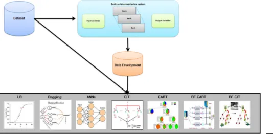
The framework starts with DEA computation of the performance of each bank, and the efficiency scores obtained are grouped accordingly into efficient banks (efficiency score of 1, target = 1) and inefficient banks (efficiency score less than one, target = 0). This classified efficiency score is used as a target, while the environmental (exploratory) variables are used as inputs of data mining techniques.Figure 1depicts our proposed framework.
In the following paragraphs, we briefly describe the DEA and the seven prediction techniques used in our study.
3.1 Data envelopment analysis
DEA is a non-parametric method developed by Charnes et al. (1978) to measure the performance of set decision-making units (DMUs) (Emrouznejadet al., 2008andEmrouznejad and De Witte, 2010). The initial DEA models consider constant return to scale (CRS) which ignores the fact that different DMUs (banks) could be operating at different scales. To overcome this drawback,Bankeret al.(1984)introduced variable returns to scale (VRS) model,
Figure 1. DEA/data mining methodology for MENA countries commercial banks
Data
envelopment
analysis
171
which ensures that each bank is only benchmarked against banks of similar size. To introduce DEA-VRS model, assume there arenbanks (aj= 1,. . .,n) using m inputs (xiji= 1,. . .,m) and
producing s outputs (yrj, j= 1,. . .,s). DEA measures the technical efficiency of bank j0compared tonpeer group of banks input and output. DEA formulation in Models (1a) assesses bankj0 under VRS, where the efficiency of bankj0is the optimal value ofu. This model is described as input oriented. Similarly, an output-oriented DEA is defined in Model (1b) where the efficiency of bankj0is the optimal value of 1=1(Thanassoulis, 2001).
Model 1a. Standard input-oriented DEA-VRS Minu subject to Xn j¼1 ljxij#uxij0 ;8i Xn j¼1 ljyrj yrj0 ;8r Xn j¼1 lj¼1 lj 0 ;8j;ufree
Model 1b. Standard output-oriented DEA-VRS Max1 subject to Xn j¼1 ljxij#xij0 ;8i Xn j¼1 ljyrj hyrj0 ;8r Xn j¼1 lj¼1 lj 0;8j;1free
To reach to CRS-DEA, one can removePnj¼1lj51 constraint from the above models.
IMEFM
12,2
However, DEA alone determines only the efficiency scores of each bank and does not account for the factors related to inefficiency; neither can it predict the performance of each bank (Emrouznejad and Anouze, 2010) nor account for flexible measures variables (Amirteimoori and Emrouznejad, 2011; Amirteimoori and Yan, 2014) and the uncertain nature of the future (Amirteimooriet al., 2013).
3.2 Logistic regression
LR is a generalization of linear regression (Hosmer and Lemeshow, 2000) used for predicting a dichotomous dependent variable (efficient, inefficient) or multi-class-dependent variables. LR assumes that the response variable is linear in the coefficients of the predictor variables. In this study, LR analysis is performed withfinancial and economic data related to bank performance to assess the independent effect of each factor. The specific form of a logistic model is as follows:
probabiltyðefficientjx1;. . .;xmÞ5
1
1þeðb0þb1x1þ...þbkxmÞ
wherex1;...;xmaremexplanatory variables. LR produces a simple probabilistic formula of
classification, and this is its main advantage. However, the weakness is that LR cannot deal with the problems of non-linear and interactive effects of explanatory variables (Yeh and Lien, 2009).
3.3 Classification and regression tree
A classification and regression tree is a non-linear discrimination method that uses a set of independent variables to split a sample into progressively smaller subgroups. Tree-based methods have appeared with Morgan and Sonquist (1963). However, they gained their popularity through the major theoretical and practical contribution ofBreimanet al.(1984). It was initially introduced as an alternative to parametric methods in discriminant and regression analysis and has been extended more recently to censored survival analysis (LeBlanc and Crowley, 1992;Bou-Hamadet al., 2009;Bou-Hamadet al., 2011). CART uses a recursive algorithm to split the data into classes (or nodes) based on logical if-then conditions on the explanatory variables. The splitting criteria of classification trees aim to find the best splitter explanatory variable portioning the parent node into two more homogenous children nodes. The algorithm starts with the root node (initial data set) and so on until growing a large tree. For classification trees, the goodness of the split is measured by the impurity function defined as follows:
Dð Þ ¼s;t i tð Þ pLi tð Þ L pRi tð ÞR
wheresis the candidate split of a variable (v, t) the parent node,i tð Þthe impurity of the nodet pLandpRthe proportions of objects going to the leftð ÞtL or rightð ÞtR child nodes, respectively,
andi tð ÞL andi tð ÞR their impurities. Several impurity measures have been proposed, and the
most popular ones are the deviance and the Gini index. The impurity measure is defined as i tð Þ5 Pcj¼1pjð Þt ln pjð Þt
for the deviance andi tð Þ51Pcj¼1 pjð Þt
2
for the Gini index, wherepjð Þt is the proportion of objects in nodeð Þt that belong to thejthclass of theð ÞC classes
present in the data set.
The growth of the tree can be continued until no further splits are possible. However, fully grown trees tend to over-fit the data, which is why a stopping criterion is needed.
Data
envelopment
analysis
Breimanet al.(1984), proposed a pruning algorithm in which a large tree is grown then pruned back to produce a set of nested trees from which thefinal tree will be selected.
The main advantage of classification trees is the simplicity of interpreting their results. Another advantage is that classification trees do not require implicit assumptions as in the case of parametric models. Despite their advantages, decision trees suffer from instability (Breimanet al., 1984), where a small change in the training data may have a major impact on the predictive ability of the tree.
3.4 Conditional inference trees
Unlike CART where its splitting criterion is based on impurity reduction, the CIT recently proposed byHothornet al.(2006b)use a splitting criterion based on multiplicity-adjusted conditional tests (Hothornet al., 2006a). For any node, the splitting procedure consists of conducting a global permutation test of no association between any predictor variable and the response within the node. If the global hypothesis of no association is not rejected, the node is not split and is considered a terminal node. Otherwise, for each predictor, an individual null hypothesis of no association with the response will be conducted. The predictor with the lowestp-value is selected for splitting. In CIT, pruning is not required as the trees stop growing when the split is not statistically significant.
3.5 Bagging
A single tree is unstable in the sense that small perturbations in its training set may result in changes in its predictions (Breiman, 1996). Using ensemble methods such as bagging and random forests often produces better performances than using a single tree. Bagging is a bootstrap ensemble method introduced by Breiman (1996). It can be used with many classification methods and regression methods to reduce the variance associated with prediction and therefore improve the prediction process (Sutton, 2005). Hence, it consists of averaging thefitted values of the response variable of many trees built with bootstrapped samples from the original data. Basically, it trains each classifier on a randomly drawn training set; each classifier’s training set consists of same number of banks randomly drawn from the original training set, with an equal probability of drawing any given bank. These samples are drawn with replacement so that some banks may be selected multiple times, while others may not be selected at all. As a result, each classifier could return a higher test set error than a classifier using all of the data (Kim, 2006). However; when these classifiers are combined (typically by voting), the resulting ensemble produces a lower error on the test set than a single classifier. Bagging has been found to be the simplest algorithm that helps in reducing variance and improving unstable classifiers in accuracy (Breiman, 1996). It also enhances accuracy when random features are used and can help avoid overfitting. However, the disadvantage of bagging is that bagged trees are not as easily interpretable as a single tree (Zhu, 2010).
3.6 Random forests
Breiman (2001)originally introduced the random forest as an ensemble of CART trees (RF-CART). This method gives a prediction based on the majority voting (the case of classification) or averaging (the case of regression) predictions made by each tree in the ensemble using some input data (Antipov and Pokryshevskaya, 2012). In this sense, it is similar to the bagging technique, and it combines many individual decision trees to provide a final prediction. However, the key difference between them is that bagging uses an exhaustive search of all the explanatory variables tofind the best split, while RF uses a randomly selected set of explanatory variables at this step. Recently,Stroblet al. (2007)
IMEFM
12,2
developed a random forest based on conditional inference trees (RF-CIT). The general method of both RF-CART and RF-CIT can be outlined as follows:
Draw B bootstrap samples from the data,
Grow a tree for each bootstrap sample. At each node, select at random k out of m covariates on which to base the decision at that node.
Each tree is fully grown and not pruned. The splitting is stopped when a minimum node size is reached.
RF suffers from the same problem of interpretation as bagging does. However, several techniques have been developed for RF to allow for interpretation. The most useful one is the variable importance; the common and frequently used variable importance measure is the permutation-based mean decrease in accuracy (Breiman, 2001). This measure allows researchers to identify a set of important variables that can potentially affect the dependent variable.
3.7 Artificial neural networks
ANNs are one of the most commonly used data mining models for prediction. An ANN is inspired by the structure of biological neural networks where neurons are interconnected and learn from experience. Neural networks are composed of nodes (neurons) arranged in layers that are fully connected to the preceding layer via a system of weights. Numerous different neural network architectures have been studied. However, the most successful applications of neural networks have been multilayer feed forward networks. These are networks in which there is an input layer, one or more hidden layers and an output layer. The input layer is where the input features are fed and forwarded to the hidden layer, which is again forwarded to the output layer.
The output of a hidden layer node is computed in the following manner. First, a weighted sum of inputs is computed and then a transfer function is applied to this sum. More specifically, for a set of input values,x1;x2; :::;xm, the output of nodejis computed by taking
the weighted sum ujþ
Pm i¼1
wijxi, where uj;w1j; :::;wmj are weights that are initially set
randomly and adjusted as the network learns. The next step is to apply a transfer function g to this sum. A transfer function is a monotone function. The most popular transfer function is the logistic functiong sð Þ ¼1=ð1þesÞ. Finally, the output layer obtains input values
from the hidden layer and the same transfer function is applied to create the output (Shmueli et al., 2010, pp. 222-229).
The common algorithm used to estimate and update the weights is the back-propagation (Rumelhartet al., 1986). However, this algorithm suffers from a low learning speed (Castillo
et al., 2006). Many alternatives have been proposed to increase the learning speed. One of
them is a general quasi-Newton optimization procedure, the Broyden-Fletcher-Goldfarb-Shanno algorithm that is used in this paper.
4. Data description
The proposed methodology is applied to a sample of banks operating in MENA countries over the period of 2008-2010. The period after 2011 was witness an Arabic Spring movement that impacted the performance of banking sector in these countries; therefore, these years were excluded to avoid any up-normal variation in bank performance. The total number of banks operating in MENA countries over the selected period was 535 banks, however due to data availability only 151 banks (Appendix A) are included. The sample includes data from
Data
envelopment
analysis
Lebanon (27 banks); Egypt (21); United Arab Emirates (18); Bahrain; Israel and Jordan (13 banks each); Saudi Arabia (11); Oman (7); Qatar and Tunisia, (6 banks each); Iran and Kuwait (5 banks each); Algeria (2) and Libya; Morocco; Yemen and Palestine (1 bank each). Figure 2illustrates their share of assets.
Although our sample consists of banks from various countries with differing accounting regulations, we believe the accounting data are comparable across the whole sample, as the financial statements data optioned from Bankscope are reported in a unified global format. 4.1 Data envelopment analysis input and output variables
In general, different set of input and output variables were used in various studies. A debatable concern usually occurs when it comes to classifying a variable as either an input or an output due to varying definitions. There are three main approaches used as a base to select and classify the input and output variables: production, intermediate and value-added approach. Other researchers used a mix approaches. Thefirst approach popular in branches efficiency studies was that bank is treated as a vendor who use labor, capital and equipment to produce various number of deposits and loans transactions. The second approach treats banks as intermediaries between savers and investors, hence variables such as labor or labor cost and deposits and assets were frequently used as inputs and variables like loans, securities and investments were frequently used as outputs.
In this study, for the purpose of measuring bank performance and comparing different data mining techniques in predicting the performance, an in-depth analysis of previously published literature was conducted to select the most popular input and output variables. A total of 204 published were reviewed and analyzed in term of used inputs, output and environmental variables. In term of DEA input and output variables, most of the reviewed literature relied on bank’s balance sheet.Figure 3illustrates the most used input variables, whereasFigure 4illustrates the most used DEA output variables andTable IIillustrates the most used environmental variables and the used statistical test to study the impact of the environmental variables on bank performance.
Figure 3 shows the most popular DEA input variables are fixed assets, personnel expenses and number of employees, operational (interest) expense, overhead expenses, number of branches, premises and deposits. However, due to data availability and high correlation between personnel expenses and number of employees; therefore, personnel expenses withfixed assets, deposit and equity are selected as a DEA input variable.
Figure 2. Share of assets, MENA countries commercial banks
IMEFM
12,2
176
On the other hand,Figure 4shows the most popular DEA output variables that extracted from the reviewed literature.
Figure 4shows that loans is the most used output variable followed by investment, other earning assets, net commission, profit and off-balance sheet items. However, due to data availability the following outputs are selected loans, net income (profit), off-balance sheet and liquid assets.
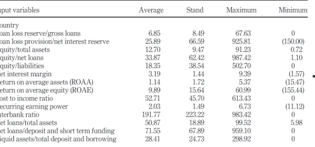
A brief statistical descriptive of DEA input and output variables are presented inTable I. On the other hand,Table IIIdescribes the 15 environmental variables considered for the second stage, as inputs to data mining algorithms.
Table Ishows that DEA model consists offive inputs and four outputs. These variables vary over the study period: the minimum value offixed assets, which is one of the inputs, is US$0.16m, whereas the maximum value is US$2,424.24m, with an average of US$143.83m and standard deviation of US$305.39m. In terms of loans, which are output variables, the minimum loan is US$1.28m, and the maximum value is US$58,487.64m, with an average of US$6,052.46m and standard deviation of US$9,702.11m. Therefore, as DEA models are sensitive to observations, it is likely tofind significant levels of variation in the efficiencies as well. Figure 4. Summary of used output variables in the reviewed literature Figure 3. Summary of used input variables in the reviewed literature
Data
envelopment
analysis
4.2 Determinants of bank efficiency: select data mining input variables
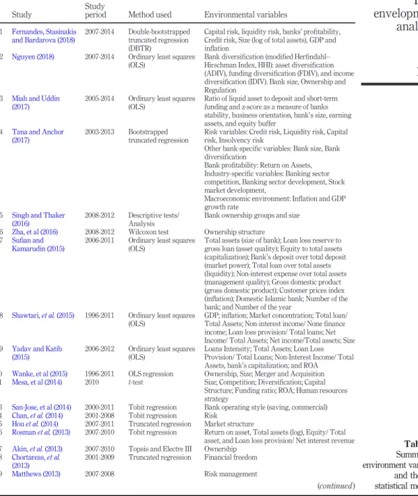
Although, measuring bank efficiency score can vary according to managerial decisions, the impact of environmental variables has been highlighted by previous research because of its effect on these decisions.Table IIsummarizes part of the previously published studies in thisfield along with the statistical methods used to investigate the impact of environment variables on bank performance.
Table IIpresents keyfindings of previous studies that investigated the impact of different exogenous variables on banks efficiency and the used statistical test. It is clear from this table that these studies used different environmental variables, and the majority of researchers used regression analysis. Few of them used other techniques such as classification and regression and data mining techniques. Introducing such methods to the study of bank performance was motivated by the need to avoid some of the critical problems in regression analysis by avoiding parametric assumptions, reducing dimensionality of the model and removing the redundant variables, which is in favor of the model’s performance. Moreover, selecting the most important variables with good predictive capacities will allow us to interpret the parameter estimates easily due to a plausible reduction of multicollinearity. Based onTable IIand data availability, Table IIIillustrates the statistical description of the selected environmental variables.
5. Experimental setup
This section describes the data used for training and testing the model, the adjustable parameters for each data mining technique and the predictive performance measures used.
5.1 Data partition and parameters
Using the statistical programming language R, which is widely used among statisticians, all predictor variables are included as inputs, and the efficiency class (0 or 1) obtained from DEA is also included as output. Then the initial data set is partitioned into training and validation data sets. The training data set contains all of the bank data over the two years 2008 and 2009, while the data set of 2010 is used for testing. The adjustable parameters of each class have been set. The bagging and the two types of random forests (RF-CART and RF-CIT) are built with 50 bootstrap samples. For neural networks, one hidden layer with five neurons is used. The splitting criterion used in CART is the deviance. The minimum number of observations in a node isfixed to 10. For CIT, the significance level of the permutation tests is set to 5 per cent. The deletion or inclusion of an explanatory variable in the logistic model is based on Akaike’s information criterion.
Table I.
Statistical descriptive of input and output variables (US$m)
Description Average SD Maximum Minimum
Inputs Fixed assets 143.83 305.39 2,424.24 0.16 Deposits 8,628.96 12,543.11 67,599.47 2.11 Equity 1,115.05 1,675.85 8,229.41 4.95 Interest expense 285.25 404.57 2,569.13 0.12 Personnel expenses 88.06 174.25 1,252.50 0 Outputs Loans 6,052.46 9,702.11 58,487.64 1.28 Net income 140.28 286.27 1,804.59 0 Off-balance sheet 3,522.14 7,217.32 68,429.57 0 Liquid assets 2,457.64 3,603.58 26,637.08 2.31
IMEFM
12,2
178
Study
Study
period Method used Environmental variables
1 Fernandes, Stasinakis and Bardarova (2018)
2007-2014 Double-bootstrapped truncated regression (DBTR)
Capital risk, liquidity risk, banks’profitability, Credit risk, Size (log of total assets), GDP and inflation
2 Nguyen (2018) 2007-2014 Ordinary least squares (OLS)
Bank diversification (modified Herfindahl– Hirschman Index, HHI): asset diversification (ADIV), funding diversification (FDIV), and income diversification (IDIV). Bank size, Ownership and Regulation
3 Miah and Uddin (2017)
2005-2014 Ordinary least squares (OLS)
Ratio of liquid asset to deposit and short-term funding and z-score as a measure of banks stability, business orientation, bank’s size, earning assets, and equity buffer
4 Tana and Anchor (2017)
2003-2013 Bootstrapped truncated regression
Risk variables: Credit risk, Liquidity risk, Capital risk, Insolvency risk
Other bank-specific variables: Bank size, Bank diversification
Bank profitability: Return on Assets, Industry-specific variables: Banking sector competition, Banking sector development, Stock market development,
Macroeconomic environment: Inflation and GDP growth rate
5 Singh and Thaker (2016)
2008-2012 Descriptive tests/ Analysis
Bank ownership groups and size
6 Zha, et al (2016) 2008-2012 Wilcoxon test Ownership structure 7 Sufian and
Kamarudin (2015)
2006-2011 Ordinary least squares (OLS)
Total assets (size of bank); Loan loss reserve to gross loan (asset quality); Equity to total assets (capitalization); Bank’s deposit over total deposit (market power); Total loan over total assets (liquidity); Non-interest expense over total assets (management quality); Gross domestic product (gross domestic product); Customer prices index (inflation); Domestic Islamic bank; Number of the bank; and Number of the year
8 Shawtari,et al.(2015) 1996-2011 Ordinary least squares (OLS)
GDP; inflation; Market concentration; Total loan/ Total Assets; Non-interest income/ Nonefinance income; Loan loss provision/ Total loans; Net Income/ Total Assets; Net income/Total assets; Size 9 Yadav and Katib
(2015)
2006-2012 Ordinary least squares (OLS)
Loans Intensity; Total Assets; Loan Loss Provision/ Total Loans; Non-Interest Income/ Total Assets, bank’s capitalization; and ROA
10 Wanke, et al (2015) 1996-2011 OLS regression Ownership, Size; Merger and Acquisition 11 Mesa, et al (2014) 2010 t-test Size; Competition; Diversification; Capital
Structure; Funding ratio; ROA; Human resources strategy
13 San-Jose, et al (2014) 2000-2011 Tobit regression Bank operating style (saving, commercial) 14 Chan,et al.(2014) 2001-2008 Tobit regression Risk
15 Houet al.(2014) 2007-2011 Truncated regression Market structure
16 Rosmanet al.(2013) 2007-2010 Tobit regression Return on asset, Total assets (log), Equity/ Total asset, and Loan loss provision/ Net interest revenue 17 Akin,et al.(2013) 2007-2010 Topsis and Electre III Ownership
18 Chortareas,et al.
(2013)
2001-2009 Truncated regression Financial freedom
19 Matthews (2013) 2007-2008 Risk management
(continued)
Table II.
Summary of environment variables and the used statistical methods
Data
envelopment
analysis
Study
Study
period Method used Environmental variables
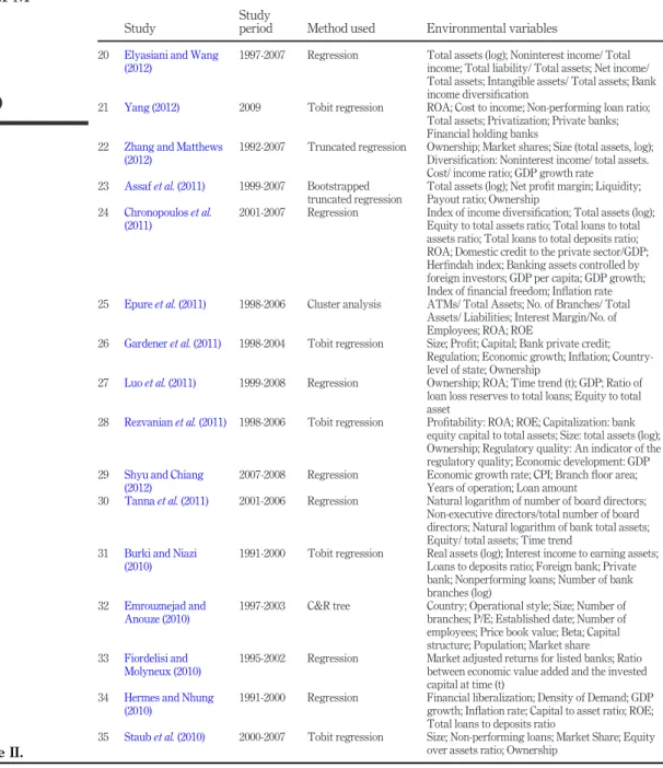
20 Elyasiani and Wang (2012)
1997-2007 Regression Total assets (log); Noninterest income/ Total income; Total liability/ Total assets; Net income/ Total assets; Intangible assets/ Total assets; Bank income diversification
21 Yang (2012) 2009 Tobit regression ROA; Cost to income; Non-performing loan ratio; Total assets; Privatization; Private banks; Financial holding banks
22 Zhang and Matthews (2012)
1992-2007 Truncated regression Ownership; Market shares; Size (total assets, log); Diversification: Noninterest income/ total assets. Cost/ income ratio; GDP growth rate
23 Assafet al.(2011) 1999-2007 Bootstrapped truncated regression
Total assets (log); Net profit margin; Liquidity; Payout ratio; Ownership
24 Chronopouloset al.
(2011)
2001-2007 Regression Index of income diversification; Total assets (log); Equity to total assets ratio; Total loans to total assets ratio; Total loans to total deposits ratio; ROA; Domestic credit to the private sector/GDP; Herfindah index; Banking assets controlled by foreign investors; GDP per capita; GDP growth; Index offinancial freedom; Inflation rate 25 Epureet al.(2011) 1998-2006 Cluster analysis ATMs/ Total Assets; No. of Branches/ Total
Assets/ Liabilities; Interest Margin/No. of Employees; ROA; ROE
26 Gardeneret al.(2011) 1998-2004 Tobit regression Size; Profit; Capital; Bank private credit; Regulation; Economic growth; Inflation; Country-level of state; Ownership
27 Luoet al.(2011) 1999-2008 Regression Ownership; ROA; Time trend (t); GDP; Ratio of loan loss reserves to total loans; Equity to total asset
28 Rezvanianet al.(2011) 1998-2006 Tobit regression Profitability: ROA; ROE; Capitalization: bank equity capital to total assets; Size: total assets (log); Ownership; Regulatory quality: An indicator of the regulatory quality; Economic development: GDP 29 Shyu and Chiang
(2012)
2007-2008 Regression Economic growth rate; CPI; Branchfloor area; Years of operation; Loan amount
30 Tannaet al.(2011) 2001-2006 Regression Natural logarithm of number of board directors; Non-executive directors/total number of board directors; Natural logarithm of bank total assets; Equity/ total assets; Time trend
31 Burki and Niazi (2010)
1991-2000 Tobit regression Real assets (log); Interest income to earning assets; Loans to deposits ratio; Foreign bank; Private bank; Nonperforming loans; Number of bank branches (log)
32 Emrouznejad and Anouze (2010)
1997-2003 C&R tree Country; Operational style; Size; Number of branches; P/E; Established date; Number of employees; Price book value; Beta; Capital structure; Population; Market share 33 Fiordelisi and
Molyneux (2010)
1995-2002 Regression Market adjusted returns for listed banks; Ratio between economic value added and the invested capital at time (t)
34 Hermes and Nhung (2010)
1991-2000 Regression Financial liberalization; Density of Demand; GDP growth; Inflation rate; Capital to asset ratio; ROE; Total loans to deposits ratio
35 Staubet al.(2010) 2000-2007 Tobit regression Size; Non-performing loans; Market Share; Equity over assets ratio; Ownership
Table II.
IMEFM
12,2
Table III. Statistical description of the environmental factors
Input variables Average Stand Maximum Minimum
Country
Loan loss reserve/gross loans 6.85 8.49 67.63 0
Loan loss provision/net interest reserve 25.89 66.59 925.81 (150.00)
Equity/total assets 12.70 9.47 91.23 0.72
Equity/net loans 33.87 62.42 987.42 1.10
Equity/liabilities 18.35 38.54 502.70 0
Net interest margin 3.19 1.44 9.39 (1.57)
Return on average assets (ROAA) 1.14 1.72 5.37 (15.47)
Return on average equity (ROAE) 9.89 15.64 60.99 (155.44)
Cost to income ratio 52.71 45.70 613.43 0
Recurring earning power 2.03 1.49 6.73 (11.12)
Interbank ratio 191.77 223.22 983.42 0
Net loans/total assets 50.87 18.89 99.52 5.98
Net loans/deposit and short term funding 71.55 67.89 959.10 0
Liquid assets/total deposit and borrowing 28.41 24.73 298.92 0
Notes:Country: organized in alphabetic order;
Asset quality
Loan loss reserve/gross loans: indicates how much of the total portfolio has been provided for but not charged off. The higher the ratio the poorer will be the quality of the loan portfolio;
Loan loss provision/net interest revenue: presents the relationship between provisions in the profit and loss account and the interest income over the same period. Ideally, this ratio should be as low as possible;
Capital
Equity/total assets: measures the ability of a bank to withstand losses. A declining trend in this ratio may signal increased risk exposure and possibly capital adequacy problem;
Equity/net loans: measures the equity cushion available to absorb losses on the loan book;
Equity/liabilities: is another way of looking at the equity funding of the balance sheet and is another way of looking at capital adequacy;
Operations
Net interest margin: is the net interest income expressed as a percentage of earning assets. The higher this ratio, the cheaper the funding or the higher the margin the bank is commanding. Higher margins and profitability are desirable as long as the asset quality is being maintained;
Return on average assets (ROAA) Return on average equity (ROAE)
Cost to income ratio: measures the overheads or costs of running the bank. It is a measure of efficiency although if the lending margins in a particular country are very high then the ratio will improve as a result. It can be distorted by high net income from associates or volatile trading income; Recurring earning power: measure of after tax profits adding back provisions for bad debts as a percentage of total assets. Effectively, this is a return on assets performance measurement without deducting provisions;
Liquidity
Interbank ratio: is money lent to other banks divided by money borrowed from other banks. If this ratio is greater than 100, then it indicates the bank is net placer rather than a borrower of funds in the market place, and more liquid;
Net loans/total assets: indicates what percentage of bank assets is tied up in loans. The higher this ratio the less liquid the bank will be;
Net loans/customer and short-term funding: highfigure denotes lower liquidity;
Liquid assets/total deposit and borrowing: amount of liquid assets available to borrower and depositors
Data
envelopment
analysis
5.2 Performance criteria
We used some popular measures of prediction performance frequently used in the literature. These measures are overall accuracy, sensitivity, specificity and the area under the ROC curve (AUC).Accuracyis the total number of banks (either efficient or inefficient) correctly classified over the total number of banks in the sample.Sensitivityis the total number of efficient banks correctly classified divided by the total number of efficient banks in the sample.Specificityis the total number of inefficient banks correctly classified divided by the total number of inefficient banks in the sample.
The above performance measures (accuracy, sensitivity and specificity) depend on a certain cutoff value for labeling the class, which is in general set at 0.5. However, AUC is considered as a better measure of overall performance and does not depend on any specific classification cutoff (Linget al., 2003). Thus, the higher the AUC, the better a classifier performs.
6. Results and discussion 6.1 First and second stage results
To provide an efficiency trend of MENA countries’commercial banks, one meta-frontier (common- frontier) approach is computed for all banks in all countries. This approach provides variations in the efficiency of banks over both time and space, which would not be the case if a separate frontier for each year were computed. Output and input-oriented DEA-VRS models are computed to measure the efficiency score of each bank.
Table IVshows that the overall average efficiency score is stable around 88 per cent over the study period for all banks. This suggests that by adopting best practices, MENA commercial banks can overall increase their outputs (without reducing any sources) or reduce their inputs (without losing any of their outputs) by approximately 11 to 13 per cent (i.e. 100 89 per cent and 10087 per cent). However, the potential increment in outputs from adopting best practices varies from bank to bank. In general, MENA commercial banks have the scope of producing 1.14 times (i.e.1
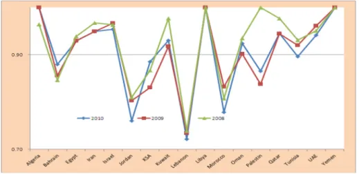
0:87) as many outputs from the same level of inputs. Furthermore, to measure bank efficiency across countries, the efficiency score for all banks is aggregated at country level to get the annual average efficiency scores for each country’s commercial banks.Figure 5illustrates the results.
Figure 5shows the Algerian, Libyan and Yemen commercial banks outperform other countries banks. On the other hand, Jordanian and Lebanese commercial banks performed badly during the study period. Thefirst stage results show the differences in inefficiency among banks in the 17 MENA countries. In this stage, the DEA results are classified into two groups, namely, efficient group (score of 1) and inefficient group (score of 0). This grouping is used as a target variable in each predictive technique. The classification or prediction performances of these techniques are presented inTable Vbased on the testing data set. It is seen that CIT outperforms the other techniques on sensitivity; however, it produced the lowest overall accuracy (67.55 per cent). RF-CART and bagging show the best overall performance with AUC of 0.9293 and 0.9221, respectively. Moreover, their estimated AUCs exhibit the lowest standard errors (S.E.).
Table IV. Summary of banks efficiency scores VRS input-oriented VRS output-oriented 2010 2009 2008 2010 2009 2008 Average 0.87 0.88 0.89 0.87 0.88 0.89 Standard division 0.15 0.15 0.14 0.16 0.15 0.14
Number of efficient banks 57 57 64 57 57 64
IMEFM
12,2
Aside from the numerical measures, the graphs inFigure 6highlight the comparison between the methods (classifiers) based on ROC curves. The ROC curve is useful for visualizing the overall performance of a classifier. It maps the sensitivity against 1 - specificity. The closer the curve is to the upper left corner, the higher the performance of the classifier.Figure 6clearly shows that RF and bagging exhibit highest performance, whereas CART, CIT and ANN exhibit the poorest performance. Thus, RF and bagging could be potentially helpful tools for predicting bank performance. However, knowing what factors affect bank performance in MENA countries might be of interest to practitioners. Therefore, RF technique is used to determine the predictors’importance in the process of predicting bank efficiency
6.2 Sensitivity analysis
For robustness purposes, we re-estimate the second-stage analysis using linear regression model using the same variables. The justification for carrying out this additional analysis is to compare the result of the best performs data mining techniques with the traditional well-known regression technique. The result of this comparison is reported inTable VI, which overall appear to corroborate the keyfindings reported in Table V and Figure 7. Specifically, we continue tofind that both RF and bagging techniques outperform the regression test. It is worth to note that regression test (LR) shows competitive performance with CART and RF-CIT on overall accuracy and specificity, but it outperforms them on sensitivity.
Figure 5. Bank performance cross MENA countries (VRS output-oriented model) Table V. Performance of the six methods
Methods Accuracy (%) Sensitivity (%) Specificity (%) AUC AUC (S.E.)
CART 75.50 52.63 89.36 0.7466 0.0408 RF-CART 82.78 68.42 90.43 0.9293 0.0194 ANN 68.21 61.40 72.34 0.6951 0.0439 Bagging 84.11 73.68 91.49 0.9221 0.0229 CIT 67.55 80.70 59.57 0.7077 0.0371 RF-CIT 75.50 52.63 89.36 0.8516 0.0306
Data
envelopment
analysis
183
6.3 Critical variables to predict bank performance
To identify the most critical environmental variables on bank efficiency and to investigate the interaction between efficiency score and the changes in the environmental variables Table VIIreports the results.
Table VIIlists the factors from the important of each variable based on RF and the significant variables based on linear regression. As Table VII, shows that both results agreed on the most important and significant variables: country, cost to income ratio and equity/net loans seem to be the most important factors in predicting bank performance, while interbank ratio and loan loss provision/net interest revenue seem to be the least important factors. This means that the performance and steady growth of thefinancial sector depend on an adequate regulatory framework. It is worth to note that these results are consistent with thefindings of recent studies byWankeet al.(2016),Liet al.(2017)and Sufian (2009)who found positive relationships between bank efficiency and equity to total assets ratio, ROA, ROE, loan loss reverse to gross loan and cost-to-income ratio.
Hence, the major concern of policymakers in countries with an inefficient banking sector need to investigate the reason for this inefficiency and learn from other countries with an efficient banking sector to improve and strengthen their financial sector. They need to understand the mechanisms of a healthyfinancial environment and help promote the health, safety and vitality of their banking sector in the coming years. The analysis also suggests that the decline in relative technical efficiency was attributed to the following many reasons such as cost-to-income ratio, equity-to-net loans ratio, equity-to-total assets ratio, loan loss reserve-to-gross loans ratio, net loan-to-deposit and short-term funding ratio and equity-to-liabilities ratio. This suggests that strong and prompt policy actions are needed to address these variables and recapitalize bank assets and cost to be more efficient.
Table VI. Performance of the seven methods
Methods Accuracy (%) AUC AUC (S.E.)
LR 74.83 0.8186 0.0348 RF-CART 82.78 0.9293 0.0194 Figure 6. Performance based on ROC curves
IMEFM
12,2
184
Take for example, the cost-to-income ratio is widely regarded as a yardstick when comparing productivity and efficiency of banks, a high cost-to-income ratio is equivalent to low productivity and low efficiency and vice versa (Burger and Moormann, 2008). Also, equity-to-net loans ratio is another important variable of bank efficiency that represent the percentage of the total assets that arefinanced by stockholders, as opposed to creditors. A low equity ratio will produce good results for stockholders as long as the company earns a rate of return on assets that is greater than the interest rate paid to creditors.
Furthermore, investors will gain more return from investing in MENA countries’banking sector if they invest their money in those countries whose banking sector is efficient. In addition, if bank managers want to open new branches in MENA countries, they are advised to open them in countries that have a healthyfinancial environment for the bank to be considered efficient. 7. Conclusion
Different statistical and data mining techniques have been used in DEA second stage to measure the impact of environmental variables on a DMU performance. Each method has its advantages and disadvantages. Most previous studies of bank performance that use the DEA second-stage approach have focused on how to explain the impact of an environmental variable on bank performance instead of predicting future bank performance. This study focused on comparing seven popular statistical and data mining techniques used in second DEA stage for bank performance to better predict bank performance in MENA countries. The techniques we used comprised CART, CIT, random forest based on CART (RF-CART), random forest based on CIT (RF-CIT) and bagging, as well as ANNs and LR. RFs and bagging have gained popularity in recent
Table VII. Variable importance obtained by RF
Variable Variable importance Linear regression*
Country 1.45 Net loan/deposit and short
term funding
Cost to income ratio 1.12 Equity/net loans
Equity/net loans 1.03 Equity/tot assets
Equity/total assets 0.99 Equity/liabilities
Loan loss reserve/gross loans
0.9 Cost to income ratio
Net loan/deposit and short term funding
0.81 Return on average equity
(ROAE)
Equity/liabilities 0.8 Loan loss reserve/gross
loans
Net loans/total assets 0.79 Cost to income ratio
Return on avg. equity (ROAE)
0.76 Country
Recurring earning power 0.76
Net interest margin 0.75
Return on avg. assets (ROAA)
0.59 Liquid assets/total deposit
and Borrowing
0.59 Loan loss provision/net
interest revenue
0.52
Interbank ratio 0.04
Note:*Significant variables based on linear regression analysis ata#0.05
Data
envelopment
analysis
years due to their superior performance in a range of applications. However, these methods, particularly random forests based on CIT, have not been used widely to predict bank performance. We provided a comparison of performance considering several measures of prediction performance such as sensitivity, specificity, overall accuracy and the area under the ROC curve (AUC). Approximately, the seven methods showed adequate ability to model bank performance. However, the overall performance of random forests and bagging was superior. A key advantage of random forests is also the variables importance ranking. In our case, RF ranked“Country”,“Cost to income ratio” and “Equity/Net loans” as the most important factors in predicting bank performance and“Interbank ratio” and“Loan loss provision/Net interest revenue” as the least important ones. We agree that any specific data may have differentfits from different data mining techniques. In the context of bank performance prediction with a target variable (Efficiency) obtained from DEA-VRs (which is our case); RFs based on CART trees were powerful tools to predict bank performance in MENA countries. Therefore, they would be of a great benefit to practitioners and researchers in MENA countries who are interested in predicting bank performance.
The result shows that both RFs and bagging techniques are the best tools to predict bank performance using DEA-VRS model. Future research should target different data set and carefully analyze the role of their environmental and regulatory specifics in efficiency levels with other DEA models such as slack-based measure and network DEA, to predict the efficiency of DMUs. However, the availability of real data is challenging; thus, a study involving simulations of different scenarios could be an interesting topic to be explored. Furthermore, as data mining tools are sensitive to used data; hence, possible venues of future studies could also try to overcome some limitations of the current study by using other environmental variables other the one used in this study to test the robustness of RFs and bagging techniques in predicting performance.
References
Akin, A., Bayyurt, N. and Zaim, S. (2013),“Managerial and technical inefficiencies of foreign and domestic banks in Turkey during the 2008 global crisis”,Emerging Markets Finance and Trade, Vol. 49 No. 3, pp. 48-63.
Amirteimoori, A., Daneshiana, B., Kordrostamia, S. and Shahroodi, K. (2013),“Production planning in data envelopment analysis without explicit inputs”,RAIRO–Operations Research, Vol. 47 No. 3, pp. 273-284.
Amirteimoori, A. and Emrouznejad, A. (2011),“Flexible measures in production process: a DEA-based approach”,RAIRO–Operations Research, Vol. 45 No. 1, pp. 63-74.
Amirteimoori, A. and Yan, F. (2014),“A DEA model for two-stage parallel-series production processes”,
RAIRO - Operations Research, Vol. 48 No. 1, pp. 123-134.
Anouze, A.L. (2010),“Evaluating productive efficiency: Aomparative study of commercial banks in Gulf Countries”, Unpublished PhD thesis, Aston Business School, Aston University.
Antipov, E. and Pokryshevskaya, E. (2012),“Mass appraisal of residential apartments: an application of random forest for valuation and a CART-based approach for model diagnostics”,Expert Systems with Applications, Vol. 39 No. 2, pp. 1772-1778.
Ariff, M. and Can, L. (2008),“Cost and profit efficiency of Chinese banks: a non-parametric analysis”,
China Economic Review, Vol. 19 No. 2, pp. 260-273.
Assaf, A., Barros, C. and Matousek, R. (2011),“Technical efficiency in saudi banks”,Expert Systems with Applications, Vol. 38, pp. 5781-5786.
IMEFM
12,2
Azadeh, A., Saberi, M., Moghaddam, R. and Javanmardi, L. (2011),“An integrated data envelopment analysis-artificial neural network-rough set algoritm for assessment of personnel efficiency”,
Expert Systems with Applications, Vol. 38 No. 3, pp. 1364-1373.
Azen, R. and Budescu, D. (2003),“The dominance analysis approach for comparing predictors in multiple regression”,Psychological Methods, Vol. 8 No. 2, pp. 129-148.
Banker, R., Charnes, A. and Cooper, W. (1984), “Some models for estimating technical and scale inefficiencies in data envelopment analysis”,Management Science, Vol. 30 No. 9, pp. 1078-1092. Berger, A. and Humphrey, D. (1997), “Efficiency of financial institutions: international survey and
directions for future research”,European Journal of Operational Research, Vol. 98 No. 2, pp. 175-212. Bou-Hamad, I., Anouze, A.L. and Larocque, D. (2017),“An integrated approach of data envelopment analysis and boosted generalized linear mixed models for efficiency assessment”,Annals of Operations Research, Vol. 253 No. 1, pp. 77-95.
Bou-Hamad, I., Larocque, D. and Ben-Ameur, H. (2011),“Discrete–time survival trees and forests with time-varying covariates: application to bankruptcy”, Statistical Modelling: An International Journal, Vol. 11 No. 5, pp. 429-446.
Bou-Hamad, I., Larocque, D., Ben-Ameur, H.,et al. (2009),“Discrete-time survival trees”,Canadian Journal of Statistics, Vol. 37 No. 1, pp. 17-32.
Breiman, L. (1996),“Bagging predictors”,Machine Learning, Vol. 24 No. 2, pp. 123-140. Breiman, L. (2001),“Random forests”,Machine Learning, Vol. 45 No. 1, pp. 5-32.
Breiman, L., Friedman, J., Olshen, R. and Stone, C. (1984), Classification and Regression Trees, Wadsworth International Group, Belmont, CA.
Burger, A. and Moormann, J. (2008),“Productivity in banks: myths and truths of the cost income ratio”,
Banks and Bank Systems, Vol. 3 No. 4, pp. 85-94.
Burki, A. and Niazi, G. (2010),“Impact offinancial reforms on efficiency of state owned private and foreign banks in Pakistan”,Applied Economics, Vol. 42 No. 24, pp. 3147-3160.
Castillo, E., Guijarro-Berdiñas, B., Fontenla-Romero, O. and Alonso-Betanzos, A. (2006),“A very fast learning method for neural networks based on sensitivity analysis”, Journal of Machine Learning Research, Vol. 7, pp. 1159-1182.
Casu, B. and Molyneux, P. (2003),“A comparative study of efficiency in european banking”,Applied Economics, Vol. 35 No. 17, pp. 1865-1876.
Chan, S., Karim, M., Burton, B. and Aktan, B. (2014),“Efficiency and risk in commercial banking: empirical evidence from East Asian countries”,The European Journal of Finance, Vol. 20 No. 12, pp. 1114-1132. Charnes, A., Cooper, W. and Rhodes, E. (1978),“Measuring the efficiency of decision making units”,
European Journal of Operational Research, Vol. 2 No. 6, pp. 429-444.
Chortareas, G., Girardone, C. and Ventouri, A. (2013),“Financial freedom and bank efficiency: evidence from the european union”,Journal of Banking and Finance, Vol. 37, pp. 1223-1231.
Chronopoulos, D., Girardone, C. and Nankervis, J. (2011),“Are there any cost and profit efficiency gains infinancial conglomeration? Evidence from the accession countries”,The European Journal of Finance, Vol. 17 No. 8, pp. 603-621.
Courville, T. and Thompson, B. (2001),“Use of structure coefficients in published multiple regression articles: is not enough”,Educational and Psychological Measurement, Vol. 61 No. 2, pp. 229-248. Elyasiani, E. and Wang, Y. (2012),“Bank holding company diversification and production efficiency”,
Applied Financial Economics, Vol. 22 No. 17, pp. 1409-1428.
Emrouznejad, A. and Anouze, A.L. (2010), “Data envelopment analysis with classification and regression tree: a case of banking efficiency”,Expert Systems, Vol. 27 No. 4, pp. 231-246. Emrouznejad, A. and De Witte, K. (2010),“COOPER-framework: a unified process for non-parametric
projects”,European Journal of Operational Research, Vol. 207 No. 3, pp. 1573-1586.
Data
envelopment
analysis
Emrouznejad, A., Parker, B. and Tavares, G. (2008), “Evaluation of research in efficiency and productivity: a survey and analysis of thefirst 30 years of scholarly literature in DEA”,Journal of Socio-Economic Planning Science, Vol. 42 No. 3, pp. 151-157.
Epure, M., Kerstens, K. and Prior, D. (2011), “Bank productivity and performance groups: a decomposition approach based upon the luenberger productivity indicator”,European Journal of Operational Research, Vol. 211 No. 3, pp. 630-641.
Estelle, S., Johnson, A. and Ruggiero, J. (2010),“Three-stage DEA models for incorporating exogenous inputs”,Computers and Operations Research, Vol. 37, pp. 1087-1090.
Fernandes, F., Stasinakis, C. and Bardarova, V. (2018), “Two-stage DEA-truncated regression: application in banking efficiency andfinancial development”,Expert Systems with Applications, Vol. 96, pp. 284-301.
Fethi, M. and Pasiouras, F. (2010), “Assessing bank efficiency and performance with operational research and artificial intelligence techniques: a survey”, European Journal of Operational Research, Vol. 204 No. 2, pp. 189-198.
Fiordelisi, F. and Molyneux, P. (2010),“Total factor productivity and shareholder returns in banking”,
Omega, Vol. 38 No. 5, pp. 241-253.
Fried, H., Lovell, C., Schmidt, S. and Yaisawarng, S. (2002),“Accounting for environmental effects and statistical noise in data envelopment analysis”,Journal of Productivity Analysis, Vol. 17 Nos 1/2, pp. 157-174. Gardener, E., Molyneux, P. and Nguyen-Linh, H. (2011),“Determinants of efficiency in South East
Asian banking”,The Service Industries Journal, Vol. 31 No. 16, pp. 2693-2719.
Grömping, U. (2007), “Estimators of relative importance in linear regression based on variance decomposition”,The American Statistician, Vol. 61 No. 2, pp. 139-147.
Hanafizadeh, P., Khedmatgozar, H., Emrouznejad, A. and Derakhshan, M. (2014),“Neural network DEA for measuring the efficiency of mutual funds”,International Journal of Applied Decision Sciences, Vol. 7 No. 3, pp. 255-269.
Hermes, N. and Nhung, V. (2010),“The impact offinancial liberalization on bank efficiency: evidence from latin america and asia”,Applied Economics, Vol. 42 No. 26, pp. 3351-3365.
Hosmer, D. and Lemeshow, S. (2000),Applied Logistic Regression, Wiley, New York, NY.
Hothorn, T., Hornik, K., van de Wiel, M. and Zeileis, A. (2006a),“A lego system for conditional inference”,The American Statistician, Vol. 60 No. 3, pp. 257-263.
Hothorn, T., Hornik, K. and Zeileis, A. (2006b),“Unbiased recursive partitioning: a conditional inference framework”,Journal of Computational and Graphical Statistics, Vol. 15 No. 3, pp. 651-674. Hou, X., Wang, Q. and Zhang, Q. (2014),“Market structure, risk taking, and the efficiency of Chinese
commercial banks”,Emerging Markets Review, Vol. 20, pp. 75-88.
Johnson, J. and LeBreton, J. (2004),“History and use of relative importance indices in organizational research”,Organizational Research Methods, Vol. 7 No. 3, pp. 238.
Kim, Y.S. (2006),“Toward a successful CRM: variable selection, sampling, and ensemble”,Decision Support Systems, Vol. 41 No. 2, pp. 542-553.
Lai, M.-C., Huang, H.-C. and Wang, W.-K. (2011), “Designing a knowledge-based system for benchmarking: a DEA approach”,Knowledge-Based Systems, Vol. 24 No. 5, pp. 662-671. LeBlanc, M. and Crowley, J. (1992),“Relative risk trees for censored survival data”,Biometrics, Vol. 48
No. 2, pp. 411-425.
Li, Z., Crook, J. and Andreeva, G. (2017),“Dynamic prediction offinancial distress using malmquist DEA”,Expert Systems with Applications, Vol. 80, pp. 94-106.
Ling, C.X., Huang, J. and Zhang, H. (2003),“AUC: a statistically consistent and more discriminating measure than accuracy”,Proceedings of the International Joint Conferences on Artificial Intelligence, pp. 519-526. Luo, D., Yao, S., Chen, J. and Wang, J. (2011), “World financial crisis and efficiency of Chinese
commercial banks”,The World Economy, Vol. 34 No. 5, pp. 805-825.
IMEFM
12,2
Matthews, K. (2013),“Risk management and managerial efficiency in Chinese banks: a network DEA framework”,Omega, Vol. 41 No. 2, pp. 207-215.
Mesa, R., Sánchez, H. and Sobrin, J. (2014),Main Determinants of Efficiency and Implications on Banking Concentration in the European Union. Revista de Contabilidad, Vol. 17, pp. 78-87. Miah, M. and Uddin, H. (2017),“Efficiency and stability: a comparative study between Islamic and
conventional banks in GCC countries”,Future Business Journal, Vol. 3 No. 2, pp. 172-185. Morgan, J. and Sonquist, J. (1963),“Problems in the analysis of survey data and a proposal”,Journal of
the American Statistical Association, Vol. 58 No. 302, pp. 415-434.
Nguyen, T. (2018),“Diversification and bank efficiency in six ASEAN countries”,Global Finance Journal, Vol. 37, pp. 57-78.
Pedhazur, E.J. (1997),Multiple Regression in Behavioral Research, Harcourt Brace, Fort Worth. Ray, S. (1988),“Data envelopment analysis, nondiscretionary inputs and efficiency: an alternative
interpretation”,Socio-Economic Planning Science, Vol. 22 No. 4, pp. 167-176.
Ray, S. (1991),“Resource-use efficiency in public schools: a study of Connecticut data”,Management Science, Vol. 37 No. 12, pp. 1620-1628.
Rezvanian, R., Ariss, R. and Mehdian, S. (2011), “Cost efficiency, technological progress and productivity growth of Chinese banking pre- and post-WTO accession”, Applied Financial Economics, Vol. 21 No. 7, pp. 437-454.
Rosman, R., Abd Wahab, N. and Zainol. Z., (2013),“Efficiency of Islamic banks during thefinancial crisis: an analysis of Middle Eastern and asian countries”,Pacific-Basin Finance Journal, doi: 10.1016/j.pacfin.2013.11.00.
Rumelhart, D., Hinton, G. and William, R. (1986), “Learning representations of back-propagation errors”,Nature, Vol. 323 No. 6088, pp. 533-536.
San, O., Theng, L. and Heng, T. (2011),“A comparison on efficiency of domestic and foreign banks in Malaysia: a DEA approach”,Business Management Dynamics, Vol. 1, pp. 33-49.
San-Jose, L., Retolaza, J. and Pruñonosa, J. (2014),“Efficiency in spanish banking: a multistakeholder approach analysis”,Journal of International Financial Markets, Institutions and Money, Vol. 32, pp. 240-255. Seol, H., Choi, J., Park, G. and Park, Y. (2007),“A framework for benchmarking service process using data
envelopment analysis and decision tree”,Expert Systems with Applications, Vol. 32 No. 2, pp. 432-440. Shawtari, F., Ariff, M. and Abdul Razak, S. (2015),“Efficiency assessment of banking sector in Yemen
using data envelopment window analysis: a comparative analysis of islamic and conventional banks”,Benchmarking: An International Journal, Vol. 22 No. 6, pp. 1115-1140.
Shmueli, G., Patel, N. and Bruce, P. (2010),Data Mining for Business Intelligence: Concepts, Techniques, and Applications in Microsoft Office Excel with XLMiner. (2nd Ed.), Wiley, NJ.
Shyu, J. and Chiang, T. (2012),“Measuring the true managerial efficiency of bank branches in Taiwan: a three-stage DEA analysis”,Expert Systems with Applications, Vol. 39 No. 13, pp. 11494-11502. Singh, P. and Thaker, K. (2016),“Dynamics of scale efficiency of indian banks: a deterministic frontier
approach”,The Journal of Developing Areas, Vol. 50 No. 3, pp. 437-457.
Staub, R., Souza, G. and Tabak, B. (2010),“Evolution of bank efficiency in Brazil: a DEA approach”,
European Journal of Operational Research, Vol. 202 No. 1, pp. 204-213.
Strobl, C., Boulesteix, A.-L., Zeileis, A. and Hothorn, T. (2007), “Bias in random forest variable importance measures: illustrations”,Sources and a Solution, BMC Bioinformatics, Vol. 8, pp. 25. Sufian, F. (2009),“Determinants of bank efficiency during unstable macroeconomic environment: empirical
evidence from Malaysia”,Research in International Business and Finance, Vol. 23 No. 1, pp. 54-77. Sufian, F. and Kamarudin, F. (2015),“Determinants of revenue efficiency of Islamic banks: empirical
evidence from the Southeast Asian countries”,International Journal of Islamic and Middle Eastern Finance and Management, Vol. 8 No. 1, pp. 36-63.
Data
envelopment
analysis
Sun, J. and Li, H. (2008),“Data mining method for listed companies’financial distress prediction”,
Knowledge-Based Systems, Vol. 24, pp. 1-5.
Sutton, C. (2005),“Classification and regression trees, bagging, and boosting”,Handbook of Statistics, Vol. 24, pp. 303-329.
Tana, Y. and Anchor, J. (2017),“The impacts of risk-taking behaviour and competition on technical efficiency: evidence from the chinese banking industry”,Research in International Business and Finance, Vol. 41, pp. 90-104.
Tanna, S., Pasiouras, F. and Nnadi, M. (2011),“The effect of board size and composition on the efficiency of UK banks”,Int. J. of the Economics of Business, Vol. 18 No. 3, pp. 441-462.
Thanassoulis, E. (2001),Introduction to the Theory and Application of Data Envelopment Analysis: A Foundation Text with Integrated Software, Kluwer Academic, MA.
Toloo, M., Zandi, A. and Emrouznejad, A. (2015),“Evaluation efficiency of large-scale data set with negative data: an artificial neural network approach”,The Journal of Supercomputing, Vol. 71 No. 7, pp. 2397-2411.
Wanke, P., Azad, M. and Barros, C. (2016),“Predicting efficiency in malaysian Islamic banks: a two-stage TOPSIS and neural networks approach”,Research in International Business and Finance, Vol. 36, pp. 485-498.
Wanke, P., Barros, C. and Faria, J. (2015),“Financial distress drivers in Brazilian banks: a dynamic slacks approach”,European Journal of Operational Research, Vol. 240 No. 1, pp. 258-268. Wu, T.-C. and Hsu, M.-F. (2019),“Credit risk assessment and decision making by a fusion approach.
Knowledge-based systems”, available at:http://dx.doi.org/10.1016/j.knosys.2012.04.025 Yadav, R. and Katib, M. (2015),Technical Efficiency of Malaysia’s Development Financial Institutions:
Application of Two-Stage DEA Analysis,Asian Social Science, Vol. 11, pp. 175-182.
Yang, C.-C. (2012),“Service, investment, and risk management performance in commercial banks”,The Service Industries Journal, Vol. 32 No. 12, pp. 2005-2025.
Yeh, I. and Lien, C. (2009),“The comparisons of data mining techniques for the predictive accuracy of probability of default of credit card clients”,Expert Systems with Applications, Vol. 36 No. 2, pp. 2473-2480.
Zha, Y., Liang, N., Wu, M. and Bian, Y. (2016),“Efficiency evaluation of banks in China: a dynamic two-stage slacks-based measure approach”,Omega, Vol. 60, pp. 60-72, available at:http://dx.doi.org/ 10.1016/j.omega.2014.12.008i
Zhang, T. and Matthews, K. (2012),“Efficiency convergence properties of Indonesian banks 1992-2007”,
Applied Financial Economics, Vol. 22 No. 17, pp. 1465-1478.
Zhu, D. (2010),“A hybrid approach for efficient ensembles”,Decision Support Systems, Vol. 48 No. 3, pp. 480-487.
Further reading
Alandejania, M. and Asutay, M. (2017),“Nonperforming loans in the GCC banking sectors: does the islamicfinance matter?”,Research in International Business and Finance, Vol. 42, pp. 832-854. Corresponding author
Abdel Latef M. Anouze can be contacted at:[email protected]
For instructions on how to order reprints of this article, please visit our website: www.emeraldgrouppublishing.com/licensing/reprints.htm
Or contact us for further details:[email protected]
IMEFM
12,2