Exploiting Performance and Cost Diversity in the Cloud

Exploiting Performance and Cost Diversity in the Cloud

Luke M. Leslie, Young Choon Lee, Peng Lu and Albert Y. Zomaya Centre for Distributed and High Performance Computing

School of Information Technologies The University of Sydney

NSW 2006 Australia

Email:{lles9991, pelu1144}@uni.sydney.edu.au,{young.lee, albert.zomaya}@sydney.edu.au Abstract—Infrastructure-as-a-Service (IaaS) platforms, such

as Amazon EC2, allow clients access to massive computational power in the form of virtual machines (VMs) known as instances. Amazon hosts three different instance purchasing options, each with its own service level agreement covering availability and pricing. In addition, Amazon offers access to a number of geo-graphical regions, zones, and instance types from which to select. In this paper, we present a resource allocation and job scheduling framework (RAMC-DC), which utilizes Amazon’s rich selection of service offerings—particularly within Spot and On-Demand instance purchasing options—aiming to cost efficiently execute deadline-constrained jobs. The framework is capable of ensuring quality of service in terms of cost, deadline compliance and service reliability. Such capacities are realized incorporating a set of novel strategies including execution time and cost approximation, bidding and resource allocation strategies. To the best of our knowledge, RAMC-DC most extensively exploits the service diversity of Amazon EC2, and offers a comprehensive cost efficiency solution that is able to deliver both the performance and reliability of On-Demand instances and the low costs of Spot instances. Experimental results obtained from extensive simulations using Amazon’s Spot price traces show that our approach keeps deadline breaches and early-termination rates as low as 0.47% and 0.18%, respectively. This reliable performance is achieved with total costs between 13% and 20% of an equivalent approach using only On-Demand instances.

Keywords-Spot instances; Cloud provisioning; Cost efficiency

I. INTRODUCTION

Cloud computing provides a means to acquire pay-as-you-go computing power and data storage in a manner similar to publicly available utilities such as gas and electricity. As such, cloud computing has become a very powerful and popular tool among users who require access to computational resources and data storage without the fixed costs involved in purchasing, installing, and maintaining a private cloud. Moreover, cloud computing providers are in a prime position to leverage economies of scale unavailable to users with small private clouds, and therefore can pass these savings on to the users. There are many different cloud computing providers and each offers different layers of services. The focus in this paper will be on IaaS providers, specifically Amazon EC2.

Amazon EC2 offers three different instance purchasing options. These are: reserved instances, where a user pays a yearly fee and receives a discount on hourly rates; On-Demand instances, where a user pays a single hourly rate; and Spot instances, where users bid for instances [1]. While Spot instances benefit from low costs, they also suffer from inherent volatility. On the other hand, On-Demand instances offer very

low volatility but higher prices than equivalent Spot instances. Taking advantage of this apparent dichotomy provides an attractive path to achieving both high cost-efficiency and low volatility. As in the Pinterest example,1 _{supplementing Spot} instances with On-Demand instances can help reduce the volatility encountered by the application and lower total costs. There have been several previous studies aimed at cre-ating resource allocation strategies utilizing Spot instances. Examples such as BROKER [3], SRRP and DRRP [4], and that introduced in [5], all seek to simply provision Spot instances to run computations. Among such strategies, only [3] incorporates the use of different types of Spot instances from separate availability zones, but compares only cost efficiency across these zones, rather than the inherent reliability of each. In this paper, we present a resource allocation and job scheduling framework (RAMC-DC) that exploits performance and cost diversity in order to schedule deadline-constrained jobs on a dynamic cluster of Spot and On-Demand instances. RAMC-DC is unique in that it compares price dynamics from different purchasing options, instance types, and availability zones, and evaluates comprehensive methods to estimate the cost of execution on a Spot instance and different checkpoint-ing strategies. Furthermore, our approach provides biddcheckpoint-ing and resource allocation strategies designed to examine:

i theinterchangeability of an instance among short jobs, ii theprobability of completionof long jobs on an instance, iii thetradeoffs of using an On-Demand or Spot instance, iv and thecost effectivenessof running jobs on an instance.

Experimental results using Amazon’s Spot prices from the period between July and November 2012, and using Downey’s speedup model [6] show that our approach can keep total costs between 13% and 20% of the equivalent cost when using only On-Demand instances. Furthermore, these cost savings are achieved while maintaining early-terminations and deadline breaches as low as 0.18% and 0.47%, respectively.

The remainder of this paper is organized as follows. Section II describes background and related work. Section III outlines the instance and job models, and the overall problem RAMC-DC attempts to solve. Section IV introduces the checkpointing strategies, and develops and evaluates comprehensive cost ap-proximation methods. Section V presents the dynamic resource

1_{The content provider Pinterest was able to reduce its costs from $54/hr to}

$20/hr by using a dynamic combination of Spot and On-Demand instances (targeted to generally be 50-50) to handle elastic load [2].

12:00 14:24 16:48 19:12 21:36 00:00 02:24 04:48 07:12 09:36 12:00 0 0.2 0.4 0.6 0.8 1 1.2 1.4 1.6 1.8 2 Time (HH:MM)

Spot Price ($US)

us−east−1a us−east−1b us−east−1c us−east−1d us−east−1e On−Demand

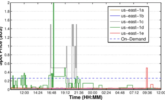
Fig. 1: Spot prices for instance typem1.large, running a Linux OS, for all availability zones in regionus-east-1.

provisioning strategy as the primary component of RAMC-DC, and an evaluation of RAMC-DC is given in Section VI. The conclusions are then drawn in Section VII.

II. BACKGROUND ANDRELATEDWORK

In this section, we begin by describing Amazon’s service diversity, with a focus on Spot instances. We then discuss pre-vious studies as they relate to bidding and resource allocation strategies for Spot instances.

A. Spot Instances

Amazon offers their IaaS instances in three different ways with different price and availability/reliability dynamics. Much of the diversity in these offerings is within Spot instances. Each Spot instance type is available in certain zones through a Spot market in which users bid for instances. This Spot market has an associated time-varying price which determines the cost of running a user’s Spot instance, as well as if and when the instance is terminated by Amazon. If the user’s bid exceeds the current market price, the user gains access to the instance as long as this holds true, with the user being charged the current market price at the start of each hour block. If the market price exceeds the bid, the instance is terminated by Amazon and the user is not charged for that partial hour. An example of these market prices is shown in Figure 1. B. Bidding Strategies

Andrzejak et al. [7] present bidding strategies based on the execution times of an instance for jobs requiring 1,000 minutes of execution that were designed to satisfy SLA constraints. Zafer, Song, and Lee [8], [9] developed optimal bidding strategies in Spot markets both from a client and a broker perspective. From the client’s perspective, Zafer et al. designed a dynamic bidding policy (DBA) to minimize the total cost of a parallel or serial job with a deadline constraint. From the broker’s perspective, Song et al. develop a profit aware dynamic bidding algorithm (PADB) that maximizes the time average profit of the broker. The bidding strategies in this pa-per differ from these works and others, by allowing a trade-off between deadline breaches and total cost, adjusting the bidding

strategy depending on the execution time, and comparing the price dynamics across availability zones. Furthermore, when handling jobs with low execution times, it becomes prudent to acquire instances with bids independent of the initial jobs to allow other jobs to fill idle hour blocks.

C. Resource Allocation Strategies

There have been a number of resource allocation strategies proposed to utilize Spot instances. Zhao et al. [4] develop deterministic and stochastic resource rental planning models (DRRP and SRRP) to minimize costs when running elastic computations on Spot instances. Chen et al. [10] attempt to model the interaction between customer satisfaction and service profit for a provider that leases Spot instances from IaaS providers. Liu [11] and Chohan et al. [12] utilize Spot instances to run MapReduce applications. Voorsluys et al. [3] propose a resource provisioning policy that encompasses two novel fault tolerance techniques aimed at decreasing the volatility of a heterogeneous cluster composed of Spot instances, including migration of VM states across availability zones. Estimates of execution times were made in a fashion similar to those in this work. Contrary to the work presented here, both [10] and [3] do not compare the pricing and reliability dynamics across markets and do not supplement Spot instances with On-Demand instances.

III. MODELS

In this section, the models used by RAMC-DC for instances and jobs are described followed by our problem formulation. A. Instances

Each job is scheduled for execution on an instance, either Spot or On-Demand, represented byν. The instanceν refers to either a to-be-leased instance or an existing instance. If ν is to-be-leased, it may be represented by the triple i, z, b, whereiis the instance type,zis the availability zone, andb is the bid. The typeiis an element of the set of all types,I, andzis an element ofZ, the set of availability zones. Not all instance types are available as Spot instances in all zones: if ν is a Spot instance,z∈Zi, whereZiis the set of all zones in which a Spot instance of typei is available. ν is an On-Demand instance if and only ifb=∅; otherwise,ν is a Spot instance andb ∈ R+. When an instance is leased, a pointer

to the EC2 instance is added toν to retrieve data such as the status of the instance and the time remaining in the hour. B. Jobs

Users submit a job, j, which is placed in an FIFO queue, J. Each job is independent and includes a desired instance type,ij, an estimated execution time,t(given in full or partial hours), and a deadline, D. In the event of termination, j also contains a reference to the last zonej was executed in, zj (initially ∅). The execution time of a job most likely is dependent on the assigned instance. Such variation will be facilitated by anexample model of job moldabilitythat utilizes the number of EC2 compute units provided by an instance, and

the extent to which execution time is altered by them. Thus, we assume each job is one of the following.

Moldable: For a job to be moldable implies that some speedup or slowdown is observed when running the job on larger or smaller instances (with respect to computational power), respectively. As an exemplar of moldability, speedup will be determined similarly to [3], using Downey’s speedup model [6], and measures the change in execution time for a job running on n processors compared to a job running on 1 processor. Downey’s model requires two additional parameters,Aandσ, which measure theaverage parallelism and thecoefficient of variance in parallelism, respectively, and generatesSU(n), the speedup of a job usingnprocessors. In this work, we calculate the estimated execution time onias:

ti=t·SU(ni)/SU(nij),

whereni is the number of EC2 Compute Units ini.

Rigid: For a job to be rigid implies that no speedup is encountered on larger instances (i.e., ti = t), and that the job will not execute on smaller instances. Therefore, rigidity requires that only instance types with ni ≥ n be used to execute the job, and these will be the only instance types incorporated in the search. Such a requirement can easily be extended to memory size, storage capacity, etc.

C. Problem Formulation

Scheduling and resource allocation decisions in RAMC-DC are made based primarily on two tunable parameters, Slb∈[0,1]andtsplit∈[0,∞). The parameterSlbspecifies an evaluation lower bound in the Spot instance bidding strategies. The value of tsplit represents a splitting parameter used to classify jobs as short or long, thereby determining the evaluation used for that job. In this paper, ift ≤ tsplit, the job is classified as short. Otherwise, the job is classified as long.Slbgenerally is used to specify how much resistance to early-termination is required for Spot instances; higher values ofSlb generally increase the bid and thus incur higher costs but lower early-termination rates. The set of instance types searched,I, includes Amazon’sm1,m2,m3,c1, andcc1types. For each job in the queue, RAMC-DC must locate a job-instance (j, ν) assignment that minimizes the cost, C(j, ν), of running a job j on an instance ν, while meeting either reliability or availability constraints, depending on whether a job is classified asshortorlong(i.e., ift≤tsplit). Thus, given a job j, RAMC-DC searches among Spot and On-Demand instances to find the instanceν∗such that:

ν∗= arg min

ν∈V C(j, ν).

Here,V is a set of leased and to-be-leased instances such that

∀ν∈V, j can be executed onν before DandS(j, ν, tsplit)≥ Slb, where S(j, ν, tsplit) ∈ [0,1] is an evaluation of the assignment(j, ν)using the parametertsplit.

IV. COSTAPPROXIMATION

The cost of running a job on a particular instance is a function of job execution time and unit cost of resource rental

(hourly rate in Amazon EC2’s case). Because we adopt check-pointing to improve reliability, the checkcheck-pointing overhead needs to be taken into account when calculating job execution time. In the meantime, resource rental cost when dealing with Spot instances is subject to change and should be estimated.

In this section, we present three checkpointing strategies incorporated by RAMC-DC. Following this, we compare and evaluate five different methods for approximating the cost of execution on Spot instances.

A. Checkpointing Strategies

For some availability zone, z, the execution time in z is modified to include the estimated checkpointing times of the job, if run on a Spot instance, and the time to resume the job from a suspended state if the job was previously checkpointed:

ti,z=ti+tchkpti +treszj→z.

Here, both the estimated checkpointing time, and the resume time,treszj→z, of an instance in zonez from some checkpoint

in j’s last zone zj, are determined as in [3], [13], where the suspend and resume rates of a VM state in the same availability zone ares= 63.67M B/sandr = 81.27M B/s, and the resume rate from a different availability zone is set to r/2. Thus, the time per checkpoint is the time required to save the instance’s memory to a global file system (e.g., Amazon S3), and is given as tsusp_i = mi/s where mi is the size of the instance’s memory. Similarly, the time to resume a check-pointed instance state is calculated astres_zj→z=mi/rifz=zj, and tres_zj→z = mi/(r/2) otherwise. When resuming instance states on On-Demand instances, we lettres_OD =tres_zj→zj =mi/r, as we assumezalways equals zj in such cases.

To provide fault-tolerance, the following checkpointing strategies are compared when running jobs on Spot instances. 1) None: No checkpoints are taken. The estimated check-pointing time istchkpt_i = 0 and, upon forced termination, all completed computation is lost, forcing the job to be restarted. 2) Hourly: A checkpoint is taken at the end of each hour block. The estimated checkpointing time is therefore calcu-lated as tchkpti = ti ·tsuspi and, upon forced termination, execution resumes from the end of the last hour.

3) Rising Market Price: A checkpoint is taken each time the market price rises for that instance. Thus, we determine the estimated number of checkpoints as the average number of price increases for atiperiod over some Spot market window, and the checkpointing time istchkpt_i =avg incr·tsusp_i . B. Execution Costs

For each type-zone pair (i, z), RAMC-DC has access to Amazon’s Spot price history for some past span of time:

Hi,z={(p1, d1), . . . ,(pk=pmkt, dk)}, wherepi is the price

at time di, andpk is the current market price. To determine the best way to estimate the cost of execution, we evaluate the following five different methods for approximating the cost.

1) Market Price (mkt): The cost is approximated as the current market price (pmkt) times the ceiling oft:

2) Monte Carlo (mc): The cost is approximated using a nonparametric Monte Carlo estimate:

Cmc(j, ν) = 1 |XC| x∈XC Cx(j, ν),

whereXCis a set of 10,000 dates sampled uniformly over the past 60 days andCx(j, ν)is the true cost of running the job at timex if the job completes successfully, and is otherwise equal toCmkt(j, ν).

3) Average Price (avg): The cost is approximated using an average per-hour price calculated as the weighted sum of all previous market prices less than the bid over the past 60 days, with each weight proportional to the fraction of the time spent at each market price:

Cavg(j, ν) = pm≤b,m<kpm·(dm+1−dm) pm≤b,m<k (dm+1−dm) · ti,z. 4) Market-Monte Carlo (mmc ααα): If the runtime of the

job is less than some parameter α, the estimated cost is determined using theMarket Priceestimate of the cost. Otherwise, the estimated cost is calculated as the sum of theMarket Pricemethod for the firstα hours and the Monte Carlomethod for the remaining time.

5) Market-Average (ma ααα): As in Market-Monte Carlo but using theMonte Averageestimate for the remaining time. Ifν has been leased,C(j, ν )is calculated as the total cost accounting for the fact that the remaining hour block has already been paid for. Thus, C(j, ν) approximates the cost using the estimated execution timeti,z−RemHour(ν), where RemHour(ν) is the predicted time that will remain in ν’s hour block whenjis expected to start.

The above approximations were chosen to determine the appropriate weight given to the current market price, and to evaluate the difference in accuracy between a random sampling and an averaging approach. Increasing the weight of the market price will lead to more accurate results if the inter-price time (the time between inter-price changes) is very high. When this is true, the probability of a change in market price during execution is low, so the price first encountered is likely to remain constant. Approximations utilizing the time-weighted average price will generally yield higher accuracy than random sampling when spikes are more frequent since such approxi-mation will incorporate these spikes, while random sampling has the potential to miss such spikes altogether.

C. Comparison of Cost Approximations

To determine which cost estimation method achieves the lowest relative error, simulations are run using 20,000 jobs over two months, with desired runtime uniformly sampled between 1 and 12 hours (desired computation times above 1 hour guarantee that the true cost is nonzero), and with desired type and zone also uniformly sampled. Each job is allocated a new Spot instance of the requested type, and in the requested zone. Spot price history from the regionus-east-1is used.

0 0.1 0.2 0.3 0.4 0.5 0.6 0.7 0.8 0.9 1 0 0.05 0.1 0.15 0.2 0.25 0.3 0.35 0.4

Evaluation Lower Bound (S_lb)

Relative Error ( η ) mkt mc avg mmc_avg ma_avg mmc_2 ma_2 mmc_4 ma_4

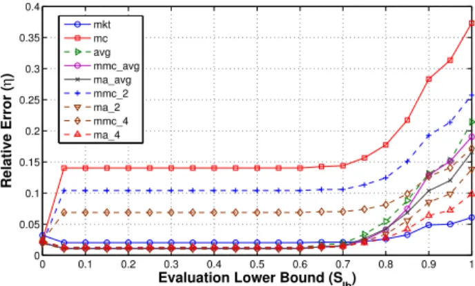
Fig. 2: A comparison of the relative error of each cost esti-mation method using availability bids with no checkpointing.

Figure 2 illustrates the accuracy of each cost estimation method for successful jobs (not terminated early) using a Slb-availability bid. Here, the variable avg represents the average inter-price time over the Spot price history for the market corresponding to (i, z). For values of Slb less than 0.7, Average, Market-Average and Market-Monte Carlo (with α=avg) approximations perform similarly, achieving relative errors of only around 0.015-0.025 each. Of the four, Market-Average withα= 4is marginally the most accurate.

For higher values of Slb, the simplest estimate, Market Price, performs the best, with other estimates quickly becom-ing more and more inaccurate asSlbincreases. This increasing disparity between cost estimates reflects the fact that other cost estimate methods rely on the instance’s potential bid. AsSlbis increased, the bid will also monotonically increase, allowing for a wider range of past market prices to be taken into account when calculating the average prices or the average costs. As Spot prices exhibit periods of little fluctuation punctuated by large price spikes, using data from periods of different market prices in the estimation will be less indicative of the actual cost. For lower values ofSlb, the range of bids which satisfy the confidence level is constricted (whenSlb= 0, the bid will always be equal to the market price) and thus cost estimation methods utilizing past Spot prices will be more accurate.

V. DYNAMICRESOURCEPROVISIONING

The overall resource provisioning process RAMC-DC em-ploys is performed by (1) evaluating instance suitability based on j’s execution time and tsplit, (2) finding the most cost-effective instance among already leased and to-be-leased in-stances that satisfy the evaluation lower bound, Slb, as well as the deadline, D, (3) leasing a new Spot or On-Demand instance if required (i.e., the optimal instance is to-be-leased), and (4) assigningjto the resulting instance.

A. Two-Tier Instance Evaluation

The suitability of an instance is determined through a two-tier instance evaluation strategy that involves the calculation of the reliability or availability of an instanceν, depending on

whether job is classified asshort orlong, and is defined as: S(j, ν, tsplit) =

Availability(ν) if t≤tsplit Reliability(j, ν) if t > tsplit , withReliability andAvailability defined below. If ν is an On-Demand instance, we assumeS(j, ν, tsplit) = 1.

Ift≤≤≤tsplit,S(j, ν, tsplit)is calculated as the portion of time thatbwas above the market price during a 60-day Spot price window for the Spot market determined by(i, z):

Availability(ν) =

pm≤b,m<k(dm+1−dm)

(dk−d1) .

As described in Section IV-B, (pm, dm) ∈ Hi,z for m =

1, . . . , k, andpk=pmkt is the current market price.

If t>>>tsplit, S(j, ν, tsplit) is calculated as the empirical probability of successful completion ifν was used to execute j. That is, Reliability(j, ν) = P(Ti,z,b≥ ti,z)where Ti,z,b is a random variable representing the true length of time for which the Spot instance is available to the user when bidding bon instance typeiin availability zonez. This probability is estimated using the nonparametric Kaplan-Meier Estimator:

Reliability(j, ν) = ti,z,b(x)≤ti,z

ni,z,b(x)−1 ni,z,b(x) , whereX is a set of 10,000 dates sampled uniformly over the past 60 days of the Spot price history,ti,z,b(x)is the true step length for an instance leased at timex∈Xwith typeiin zone z, and with bidb. Here,ni,z,b(x)is the number of samples in which the instance was available for longer thanti,z,b(x). B. Bidding

The optimal bid for a Spot instance is calculated as the minimum bid that satisfies a lower bound on the instance evaluation function described above. Thus, the bid for a Spot instance of typeiin zonezis calculated as:

b(j, i, z, tsplit) = min{b∈R+|S(j,i, z, b, tsplit)≥Slb

∧b≥pmkt(i, z)}.

If the job has an estimated execution time greater than the splitting parametertsplit, the bidding strategy locates the minimum bid such that the empirical probability of completion of j on an instance of type i in zone z is greater than or equal to Slb. Such a strategy helps to provide job-specific bids that can limit the risk of early-termination for long jobs. On the other hand, if the execution time is less than tsplit, the bidding strategy instead locates the minimum bid such that the instance has been available (i.e., the market price has been under the bid) for at leastSlb of the time over the Spot price window. This approach helps guarantee that instances areinterchangeableamong short jobs, thereby filling partially empty hour blocks.

C. Resource Provisioning

The process of resource provisioning and job assignment is described in Algorithm 1. Here,ET U I(ν)represents the

Algorithm 1: Provision - Identifying the minimum cost job-instance assignment and provisioning resources.

Data:J, Slb, tsplit 1 begin

2 SP OT ← ∅,OD← ∅ 3 whiletruedo

4 j←Pop(J)// waits for J to be non-empty 5 V ← ∅,ν∗← ∅,νnew← ∅,breach←f alse 6 Ij←i∈I :ti+tresOD≤D 7 ifIj==∅then 8 Ij← {i∈I|ni≥nj},breach←true 9 V ← {ν∈SP OT∪OD|i∈Ij∧ ETUI(ν)== 0∧S(j, ν, tsplit)≥Slb} 10 else 11 V ← {ν∈SP OT∪OD|i∈Ij∧

ETUI(ν)+ti,z≤D∧S(j, ν, tsplit)≥Slb}

12 end

13 νnew←MinNew(j, Slb, tsplit, Ij, breach)//Alg. 2

14 ν∗← arg min

ν∈V∪{νnew}

C(j, ν) 15 ifν∗==νnewthen

16 Lease(ν∗)// lease ν∗ from Amazon EC2 17 ifν∗is a Spot instancethen

18 Add(ν∗, SP OT)

19 else

20 Add(ν∗, OD)

21 end

22 end

23 Assign(j, ν∗)// pushj toν∗’s FIFO queue

24 end

25 end

estimated time until ν is idle and equals the sum of the remaining estimated runtimes of each job assigned to ν.

From the set of all instance typesI we determine the set of feasible types,Ij⊂I, that would satisfy the deadline with the corresponding On-Demand instances (line 6). If no feasible types exist,Ij is constructed as the set of instance types with ni greater than or equal to the job’s previous instance. Then, the set of allfeasible instances,V, is constructed. If there are no feasible types, as discussed above, for eachν∈V,νmust be idle and have greater than or equal to the number of EC2 compute units of the last instancejwas executed on (lines 8 and 9); otherwise, the sum of the estimated time untilνis idle and the execution time ofjonνmust be less than or equal to D(line 11). In both cases, eachνmust also satisfy the instance evaluation inequality,S(j, ν, tsplit)≥Slb. The instancevnew in line 13, identified using Algorithm 2, represents the lowest cost instance that may potentiallybe leased if no lower cost already-leased instances are found.

ν∗ is determined as the instance that minimizes the es-timated cost of execution defined by C(j, ν) (line 14). Es-timated costs for On-Demand instances are calculated as

ti,z−RemHour(ν)times the hourly On-Demand price for type i. Ifν∗is not yet leased (i.e.,ν∗==νnew as discussed

Algorithm 2: MinNew - Identifying the minimum cost new potential instance satisfyingS(j, ν, tsplit)≥Slb.

Data:j, Slb, tsplit, Ij, breach Result:νnew (an unleased instance) 1 begin

2 νnew← ∅,c∗← ∞,s∗←0 3 fori∈Ij do

4 forz∈Zi do

5 ifti,z≤D∨breachthen

6 νSP OT ← i, z, b(j, i, z, tsplit) 7 s←S(j, νSP OT, tsplit) 8 c←C(j, ν SP OT) +Cresume(j, z) 9 if(c < c∗) ∨(c==c∗∧s > s∗)then 10 νnew←νSP OT,s∗←s,c∗←c 11 end 12 end 13 end

14 νOD← i, zj,∅// potential new On-Demand

15 c←C(j, νOD)// see Section V-C 16 ifc≤c∗ then 17 νnew←νOD,s∗←1,c∗←c 18 end 19 end 20 end

above), an instance matching ν∗’s description is leased and added to the corresponding set of leased instances,SP OT or OD. Thus, ifb=∅, a Spot instance of type i, in zonez, and with bidb is leased (lines 16-18); otherwise, an On-Demand instance in zone zj is leased, where zj is eitherus-east-1aif j has not been previously attempted, or j’s last availability zone. After leasing the instance, a pointer to this instance is added toν∗ andj is then assigned toν∗’s queue.

D. Identification of New Resources

The identification ofvnew from line 13 of Algorithm 1 is outlined in Algorithm 2. The first for loop (line 3) iterates through the set of feasible instance types given by Ij, and the nestedforloop (line 4) iterates through the corresponding availability zones in which a Spot instance of typeiis avail-able. For each (i, z)combination, if the estimated execution time on type i in zone z (ti,z) satisfies the deadline, or if the job will surpass the deadline regardless, the estimated cost is compared to the current minimum. Although Amazon has since made such transfers free, if the job must be resumed from another availability zone, a data transfer cost is added at the rate of $0.01/GB ([1]) and is calculated byCresume(j, z). Due to the static pricing characteristics of On-Demand instances among availability zones, potential On-Demand instances are evaluated for each instance type only (lines 14-18).

E. Job Scheduling and Resource Deprovisioning

Ifjhas been assigned to an instance but has not been started beforeD−ti,zand the assigned instance is not idle,jis pushed

to the front ofJ. Otherwise, prior to execution, the algorithm again searches for any lower cost instances on which to run the job and reassigns the job if a cheaper alternative is found. If no cheaper alternatives are found, ij and zj are updated and j is executed. In addition to the loss of Spot instances from early-termination, On-Demand and Spot instances are automatically released at the end of the current hour block if their assignment queues are empty.

VI. EVALUATION

This section evaluates RAMC-DC through real workload traces and presents results based on total costs, deadline breaches and early-termination rates.

A. Experimental Setup

The workload used for the evaluation consists of two sets of 20,000 jobs, with execution times and arrival times taken from the traces of the ANL Intrepid supercomputer [14]. Jobs in the first set are assumed to be moldable, and jobs in the second are rigid. Each job is assumed to initially require access to a data file with size less than 1GB. Thus, jobs initially run in zones besides us-east-1a incur an additional transfer cost of $0.01. Deadlines for jobs are given as twice the estimated runtime, the requested instance type is uniformly sampled from the available types, and values ofAandσ for moldable jobs are calculated using the model of Cirne and Berman [15]. In addition, we adopt the Market Price estimation, i.e.,C=Cmkt for the sake of simplicity and accuracy. The workload traces were chosen for the general proximity of estimated and true execution times, as well as the range of these execution times, and the dispersion of jobs over a time period of several months. B. Total Costs

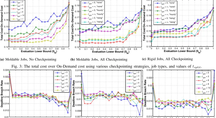
Total costs when using no checkpointing with moldable jobs are shown in Figure 3a (rigid jobs evince similar character-istics). Total costs for all checkpointing strategies and with both sets of jobs, while letting tsplit = 0 and tsplit = ∞ (as they determine upper and lower bounds), are given in Figures 3b and 3c. Thus, these two figures specify the range of observable total costs given each checkpointing strategy. Varying tsplit between these two values therefore effectively allows a tradeoff between cost and volatility, with higher values oftsplit decreasing cost but increasing volatility.

As seen in Figure 3, for all values of Slb,tsplit, and each checkpointing strategy, total costs when incorporating Spot instances are very low, attaining a minimum of 12.75% for moldable jobs and 19.5% for rigid jobs. The total costs from using only On-Demand instances in our approach are equal to $15,305 when using moldable jobs, and $24,433 when using rigid jobs. For both sets of jobs, hourly checkpointing generally incurs the highest total cost due to the checkpointing overhead. Incorporating no checkpointing strategy often results in the lowest costs, although a rising-market price strategy will achieve the lowest costs forSlb≥0.8when using rigid jobs. Allowing instance evaluation to be a function of the execution time of a job yields higher costs than evaluation relying on

0 0.1 0.2 0.3 0.4 0.5 0.6 0.7 0.8 0.9 1 0.12 0.13 0.14 0.15 0.16 0.17 0.18 0.19

Evaluation Lower Bound (S lb)

Total Cost/On−Demand Cost

t_split = 0 t_split = 3 t_split = 6 t_split = 9 t split = 12 t_split = ∞

(a)Moldable Jobs, No Checkpointing

0 0.1 0.2 0.3 0.4 0.5 0.6 0.7 0.8 0.9 1 0.12 0.13 0.14 0.15 0.16 0.17 0.18 0.19 0.2

Evaluation Lower Bound (S

lb)

Total Cost/On−Demand Cost

t_split = 0, "none" t_split = ∞, "none" t_split = 0, "hourly" t_split = ∞, "hourly" t_split = 0, "rising" t_split = ∞, "rising"

(b)Moldable Jobs, All Checkpointing

0 0.1 0.2 0.3 0.4 0.5 0.6 0.7 0.8 0.9 1 0.12 0.13 0.14 0.15 0.16 0.17 0.18 0.19 0.2 0.21

Evaluation Lower Bound (S

lb)

Total Cost/On−Demand Cost

t_split = 0, "none" t_split = ∞, "none" t_split = 0, "hourly" t_split = ∞, "hourly" t_split = 0, "rising" t_split = ∞, "rising"

(c)Rigid Jobs, All Checkpointing

Fig. 3: The total cost over On-Demand cost using various checkpointing strategies, job types, and values oftsplit.

0 0.1 0.2 0.3 0.4 0.5 0.6 0.7 0.8 0.9 1 0.01 0.012 0.014 0.016 0.018 0.02 0.022 0.024

Evaluation Lower Bound (S

lb)

Deadline Breach Rate

t_split = 0 t split = 3 t split = 6 t_split = 9 t_split = 12 t_split = ∞ (a)No Checkpointing 0 0.1 0.2 0.3 0.4 0.5 0.6 0.7 0.8 0.9 1 0.007 0.008 0.009 0.01 0.011 0.012 0.013 0.014 0.015

Evaluation Lower Bound (S

lb)

Deadline Breach Rate

t split = 0 t split = 3 t_split = 6 t_split = 9 t_split = 12 t_split = ∞ (b)Hourly Checkpointing 0 0.1 0.2 0.3 0.4 0.5 0.6 0.7 0.8 0.9 1 0.012 0.014 0.016 0.018 0.02 0.022 0.024

Evaluation Lower Bound (S

lb)

Deadline Breach Rate

t_split = 0 t_split = 3 t_split = 6 t_split = 9 t_split = 12 t_split = ∞ (c)Rising-Price Checkpointing

Fig. 4: The deadline breach rate using different checkpointing strategies and values oftsplitwith moldable jobs.

0 0.1 0.2 0.3 0.4 0.5 0.6 0.7 0.8 0.9 1 0.005 0.006 0.007 0.008 0.009

Evaluation Lower Bound (S_lb)

Deadline Breach Rate

t_split = 0 tsplit = 3 tsplit = 6 t_split = 9 t_split = 12 t_split = ∞ (a)No Checkpointing 0 0.1 0.2 0.3 0.4 0.5 0.6 0.7 0.8 0.9 1 0.005 0.0055 0.006 0.0065 0.007 0.0075 0.008

Evaluation Lower Bound (S

lb)

Deadline Breach Rate

t_split = 0 t_split = 3 t split = 6 t split = 9 t split = 12 t_split = ∞ (b)Hourly Checkpointing 0 0.1 0.2 0.3 0.4 0.5 0.6 0.7 0.8 0.9 1 0.006 0.0065 0.007 0.0075 0.008 0.0085

Evaluation Lower Bound (S

lb)

Deadline Breach Rate

t split = 0 t split = 3 t_split = 6 t_split = 9 t_split = 12 t_split = ∞ (c)Rising-Price Checkpointing

Fig. 5: The deadline breach rate using different checkpointing strategies and values oftsplit with rigid jobs. availability; total costs decrease by as much as 4% of the

total On-Demand cost when evaluation is always calculated as instance availability (tsplit=∞). Such a decrease is due to the increased interchangeability of instances, and thus the higher number of feasible instances, inherent in such an evaluation. C. Deadline Breaches

Deadline breaches generally occur very infrequently, with rates achieving a minimum of just 0.74% when using an hourly checkpointing strategy with moldable jobs, and 0.46% when using no checkpointing strategy and rigid jobs (see Figures 4 and 5). For both sets of jobs, hourly checkpointing tends to

have the lowest number of deadline breaches, and increasing Slb and decreasing tsplit tends to decrease the number of deadline breaches. However, when using moldable jobs, setting Slb= 1results in a sharp spike in deadline breaches for the noneand rising checkpointing strategies. These spikes often occur because no such instance can be found satisfyingSlb while maintaining a reasonable bid and market-price, and thus the job must wait for such an instance to become available. This additional waiting time, and sparsity of suitable instances, increases the risk and propagation of a deadline breach.

When decreasing Slb, total costs decrease and early-terminations increase. Depending on the value of tsplit and

0 0.1 0.2 0.3 0.4 0.5 0.6 0.7 0.8 0.9 1 0 0.01 0.02 0.03 0.04 0.05 0.06 0.07 0.08 0.09 0.1 0.1

Evaluation Lower Bound (S_lb)

Early−Termination Rate t_split = 0 t_split = 3 t_split = 6 t_split = 9 t_split = 12 t_split = ∞

(a)Moldable Jobs

0 0.1 0.2 0.3 0.4 0.5 0.6 0.7 0.8 0.9 1 0 0.02 0.04 0.06 0.08 0.1 0.12 0.14

Evaluation Lower Bound (S_lb)

Early−Termination Rate t split = 0 t split = 3 t split = 6 t_split = 9 t_split = 12 t_split = ∞ (b)Rigid Jobs

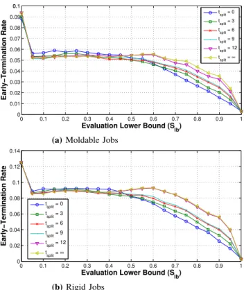
Fig. 6: Early-termination rates with no checkpointing.

the checkpointing strategy used, however, it is still possible to maintain low deadline breach rates asSlbdecreases. As seen in Figure 4b, using an hourly checkpointing strategy and letting tsplit = 0, for example, allows RAMC-DC to still maintain low deadline breaches when Slb = 0.05, while keeping the total cost equal to 13% and 14.5% of the On-Demand cost for moldable and rigid jobs. In the case of moldable jobs, a rising-market price strategy allows RAMC-DC to maintain steady deadline breach rates at around 1.6% of all jobs while incurring lower costs than an hourly checkpointing strategy. D. Early-Terminations

Early-terminations occur in as few as 0.18% of all jobs whenSlb= 1, regardless of moldability, checkpointing strat-egy, and value of tsplit (as seen in Figure 6). This figure also shows that the approach presented in this paper can keep these early-termination rates below 9.5% and 12.5% of moldable and rigid jobs, respectively, when Slb = 0. Indeed, while achieving such low early-termination rates, our approach still keeps total costs under 19.5% of the On-Demand cost, regardless of job type. The variation in early-termination rates for different values of tsplit is highest whenSlb is not equal to 0 or 1, and decrease as Slb moves to these values. For lower values of Slb (less than 0.5), all values of tsplit achieve roughly similar early-termination rates, with higher values oftsplit incurring slightly lower rates. As expected, as Slb increases, however, early-termination rates decrease until S(j, ν, tsplit) =Reliability(ν), due to the shift in focus to successful completion, rather than the reliability.

VII. CONCLUSIONS

The approach presented in this paper provides a cost ef-fective and low-volatility means to run both moldable and rigid deadline-constrained jobs. The dynamic provisioning strategy in RAMC-DC deals with the mixture of Spot and On-Demand instances, and exploits the inherent performance and cost diversity within these complementary purchasing options. Furthermore, the tunable parameters, Slb and tsplit, allow the operator to effectively trade higher total cost for lower volatility. To validate our approach, experiments were run using Amazon’s Spot price history, workload traces from ANL Intrepid with a deadline of twice the estimated runtime, and utilizing Downey’s speedup model as an exemplar approach to predicting job moldability. Our evaluation results have confirmed these claims, i.e., deadline breaches and early-termination rates are mostly below 2% and 1%, while incurring below 20% of equivalent On-Demand instance costs.

ACKNOWLEDGMENT

Prof. Zomaya would like to acknowledge the support of the Australian Research Council Discovery Grant DP1097110.

REFERENCES

[1] Amazon Elastic Compute Cloud. http://aws.amazon.com/ec2/. [2] Pinterest Cut Costs From $54 To $20 Per Hour By Automatically

Shutting Down Systems. http://tinyurl.com/azjjyn9.

[3] W. Voorsluys and R. Buyya, “Reliable provisioning of spot instances for compute-intensive applications,” inIEEE Int’l Conference on Advanced Information Networking and Applications (AINA), 2012, pp. 542–549. [4] H. Zhao, M. Pan, X. Liu, X. Li, and Y. Fang, “Optimal resource rental

planning for elastic applications in cloud market,” inIEEE Int’l Parallel and Distributed Processing Symposium (IPDPS), 2012, pp. 808–819. [5] S. Yi, A. Andrzejak, and D. Kondo, “Monetary cost-aware checkpointing

and migration on Amazon Cloud spot instances,” inIEEE Transactions on Services Computing (TSC), 2011, pp. 236–243.

[6] A. Downey, “A parallel workload model and its implications for processor allocation,” inIEEE Int’l Symposium on High Performance Distributed Computing (HPDC), 1997, pp. 112–123.

[7] A. Andrzejak, D. Kondo, and S. Yi, “Decision model for cloud com-puting under SLA constraints,” inIEEE Int’l Symposium on Modeling, Analysis and Simulation of Computer and Telecommunication Systems (MASCOTS), 2010, pp. 257–266.

[8] Y. Song, M. Zafer, and K. Lee, “Optimal bidding in spot instance market,” inIEEE Int’l Conference on Computer Communications (IN-FOCOM), 2012, pp. 190–198.

[9] M. Zafer, Y. Song, and K. Lee, “Optimal bids for spot VMs in a cloud for deadline constrained jobs,” inIEEE Int’l Conference on Cloud Computing (CLOUD), 2012, pp. 75–82.

[10] J. Chen, C. Wang, B. Zhou, L. Sun, Y. Lee, and A. Zomaya, “Tradeoffs between profit and customer satisfaction for service provisioning in the cloud,” inInt’l ACM Symposium on High Performance Distributed Computing (HPDC), 2011, pp. 229–238.

[11] H. Liu, “Cutting MapReduce cost with spot market,” in USENIX Workshop on Hot Topics in Cloud Computing (HotCloud), 2011. [12] N. Chohan, C. Castillo, M. Spreitzer, M. Steinder, A. Tantawi, and

C. Krintz, “See spot run: using spot instances for MapReduce work-flows,” in USENIX Conference on Hot Topics in Cloud Computing (HotCloud), 2010.

[13] B. Sotomayor, K. Keahey, and I. Foster, “Combining batch execution and leasing using virtual machines,” in Int’l Symposium on High Performance Distributed Computing (HPDC), 2008, pp. 87–96. [14] P. W. Archive, “Parallel Workloads Archive: ANL Intrepid,” http://www.

cs.huji.ac.il/labs/parallel/workload/l anl int/index.html.

[15] W. Cirne and F. Berman, “A comprehensive model of the supercom-puter workload,” inIEEE Int’l Workshop on Workload Characterization (WWC), 2001, pp. 140–148.