1
Joint Retirement and Leisure Time Together:
Asymmetries or Complementarities
Elena Stancanelli* and Arthur Van Soest**
April 2012
Abstract
In the scant literature on partners' joint retirement decisions one of the explanations for joint retirement is externalities in leisure. However, recent work also points to asymmetries in partners’ retirement decisions. We are not aware of any study that has tested for leisure complementarities in partners’ retirement using data on actual leisure hours together of individuals in a couple. In this study, we investigate the causal effect of retirement on partners’ hours of leisure. Our identification strategy exploits the law on retirement age in France, which enables us to use a regression
discontinuity approach to identify the effect of retirement on leisure. We find that the retirement probability increases significantly for spouses aged 60 and above, which supports our identification strategy. We conclude that own retirement increases significantly own hours of leisure. When controlling for selectivity into retirement, retirement of the husband does not increase joint leisure hours of partners, while retirement of the wife increases the couple’s joint leisure time. The evidence we gather elicits asymmetries in partners’ decisions, which is well in line with the recent literature in this area.
Keywords: Leisure, Ageing, Retirement, Regression Discontinuity
JEL classification: D13, J22, J14, C1
*CNRS, CES, University Paris 1, IZA, and OFCE, Sciences-Po **Netspar, Tilburg University, RAND and IZA
2
1. Introduction
In the scant literature on partners' joint retirement decisions one of the explanations for joint retirement is externalities in leisure. However, recent work also points to asymmetries in partners’ retirement decisions. Earlier studies of joint retirement did not explicitly consider the extent to which partners spend their leisure time together.
Here we study the causal effect of retirement on leisure hours of partners, using data that distinguish joint leisure hours from separate leisure hours of each partner. Our measure of leisure together is constructed from individual records of leisure activities reported in time use diaries where individuals also indicated with whom each activity was carried out.
Furthermore, the diary was collected from each partner on the same day, which enables us to measure hours of leisure spent separately or together.
Because individuals with stronger preferences for leisure may tend to retire earlier, we endogenize retirement in our model of joint retirement and leisure of partners. Our identification strategy exploits the law that in France, age 60 is the earliest age at which a retirement pension can be drawn. This makes each partner’s probability to be in retirement a discontinuous function of their age, with a substantial positive jump at age 60. We therefore can use a (double) regression discontinuity approach to identify the effect of own and partner’s retirement on the leisure hours of partners.
There is a scant literature on the joint retirement decisions of couples, starting from Hurd (1990). Externalities in leisure are often given as an explanation for joint retirement of both partners. A major contribution in this area is the structural dynamic model of retirement of couples developed by Alan Gustman and Thomas Steinmeier (2000), who argued that preferences for joint leisure drive joint retirement choices. However, Gustman and
Steinmeier (2009) extend this model to incorporate partial retirement strategies, and argue that in some cases individuals in a couple may decide to retire only if their partner does not retire, finding for the USA that the increased labour force participation of women has actually contributed to lower husbands’ hours of market work. This suggests that there may be asymmetries in retirement strategies of partners, which are likely to apply also to partners’ decisions concerning their leisure time together. Stancanelli and Van Soest (2012) use time
3
use data on French couples and apply a regression discontinuity approach to the retirement decisions of both partners, to investigate the causal effect of retirement on hours spent of home production, finding also evidence in asymmetry of responses of housework to partners’ retirement. In particular, they conclude that housework of the male partner increases
dramatically upon retirement, but less so when the wife also retires, while her housework is not much affected by his retirement. These studies did not explicitly consider data on hours of leisure or how much leisure the two partners spend together.
Studies on leisure hours of partners are rare and they have not investigated joint leisure in conjunction with retirement, to the best of our knowledge. In contrast, earlier literature in this area has focused on dual-earner households. Hamermesh (2002), using American data for the seventies, concluded that partners spent leisure time synchronously and that they would tend to adapt their schedules in such a way to be able to do so. Hallberg (2003), matching singles to individuals in a couple, and using Swedish time use data, investigated the effect of
working hours schedules on the fact that partners were found to consume leisure at the same time of the day, trying to disentangle what happened to be “synchronous” leisure, from leisure time that partners really ‘chose’ to spend ‘together’. He concluded that “actively” chosen joint leisure was only a small proportion of synchronized leisure.
Here we model the effect of retirement of both partners on their leisure hours endogenizing retirement of both partners. Our measure of leisure includes about 45 leisure activities ranging from watching television, to doing computer games, reading, going to the movie, visiting friends or relatives, socializing, doing sports, and going for a walk. This definition of leisure hours corresponds to a ‘narrow’ leisure definition, according, for example, to Aguiar and Hurst (2006) who studied trends in leisure hours for individuals in the United States. “Broad” leisure measures include usually any time not at work and thus, notably also house work (see also John Robinson and Geoffrey Godbey, 1997, for an excellent report on leisure issues). Here we concentrate on activities that individuals in a couple would presumably enjoy to carry out together and thus, a narrower definition of leisure applies.
We use data drawn from a time use survey for France that collects detailed diary information on the activities carried out by individuals over a full day, the same day for both individuals in a couple. The activities reported by the individuals were coded over ten minute slots and with a great detail of disaggregation; about 200 hundred activities were reported.
4
was carried out, “whom” including ‘family’ among other possibilities. Therefore, we can measure both ‘synchronous’ leisure and leisure hours ‘together’. Accordingly, we find that in our sample of couples aged 50 to 70, own leisure time on a typical day is equal to over three hours per day for husbands and about two and a half hours for women; while less than an hour and a half is spent on average on leisure activities done together. Using a “synchronous” leisure measure, about two hours are spent on average on synchronous leisure activities. Our results indicate that the retirement probability increases significantly for spouses aged 60 and above, which supports our identification strategy. Furthermore, the unobservables of the retirement equations of both partners are strongly and positively correlated with each other. We also find that own retirement significantly raises own leisure hours, while there is some evidence that partner’s retirement reduces own leisure, at least on week days –and this may be partly explained by the order of retirement, as individuals may be still at work, when their partner retires. Retirement of the wife increases the couple’s joint leisure, while the husband’s retirement reduces it, especially on week days. If retirement is treated as exogenous to the choice of hours of leisure, then both partners retirement is found to increase joint leisure hours.
This asymmetry in leisure responses of partners is well in line with the findings of Gustman and Steinmeier (2009) that partners do not always opt for retiring together. It also fits well with the evidence on substitution in partners’ house work upon both partners’ retirement, gathered by Stancanelli and van Soest (2012).
The structure of this paper is as follows. The next section presents the theoretical background and the econometric approach; Section 3 provides details of the data and the sample selection. The exploratory analysis and the results of the estimations are presented in Sections 4 and 5. Section 6 concludes.
2. A regression discontinuity approach
2.1 The theoretical framework
Models of joint retirement assume that partners have preferences for spending leisure time together and, therefore, each partner retirement decision will also be affected by the
5
retirement decision of the other partner via their preferences for spending leisure time together.
In particular, models of joint retirement, like, for instance, Gustman and Thomas Steinmeier (2000 and 2009), allow preferences for joint leisure to affect joint retirement choices by modelling each partner utility as a function of household consumption, own leisure and partner’s leisure. Moreover, Gustman and Steinmeier (2009) argue that retirement may change partners’ value of leisure.
In our framework, we allow specifically for leisure time spent together and leisure time spent separately by the two partners. When both partners are at work, leisure time together is scant while when they are both the retired, they can spend as much leisure time together as they like. Thus, it is well possible, that their marginal value of leisure falls upon retirement, and this may be also be true for the marginal value of leisure time together.
Generally, within a given couple, the husband is likely to retire earlier as he is on average older. This is especially true in countries like France where retirement age is defined by law and pension benefits are highly regulated. Now, if the husband retires first and partners have strong leisure complementarities, this will create strong incentives for the wife to retire as early as possible. In particular, since husbands are on average older than their wife, the retirement decision of the wife is likely to be more sensitive to that of the husband than
viceversa. However, Lundberg at al. (2003) suggest that the husband’s negotiation power falls when he retires from work. If this hypothesis carries over also to the wife, in dual-earner couples, when she retires her negotiation power is also likely to fall. This may generate asymmetries in retirement of partners. Changes in partners’ negotiation power upon
retirement may also affect the amount of leisure spent together or separately. The partner with more negotiation power may be the one that decides on how much of leisure time partners spend together and how much separately. Furthermore, upon retirement housework increases dramatically and especially so for the husband (as found in Stancanelli and Van Soest, 2012), which may also create asymmetries in leisure together of partners.
In conclusion, partners with stronger preferences for spending leisure time together may retire earlier than others. However, retirement may change both their bargaining power and their preferences for leisure together. Moreover, upon retirement, the amount of housework carried out by partners is likely to increase substantially. This may generate asymmetries in leisure together of partners.
6
To provide a slightly more formal outline of the theoretical set up for our RD model, let us then assume that individuals allocate their time between market work, house work and “pure” leisure subject to a budget constraint. Let m denote husbands and f wives. The husband derive utility from the household public consumption good, C, the utility derived from goods and services produced within the household, P, and the leisure time spent alone, , or together with their partner, , with the total leisure time available to the husband:
a) [(), (), () , ()] with + = Similarly, we write for wives:
b) [(), (), () , ()] with + =
For simplicity we assume that the household good is produced only with partners’ time inputs as follows, where H is the time each partner devotes to house work:
c) P=P [ + ]
Each partner maximizes their utility function subject to a budget constraint and a time constraint (there are only 24 hours a day). The budget constraint depends on the income stream from work (which is a function of the hours worked), E , and the pension benefits, B (assuming no savings for simplicity):
d) = (1 − − )+ +1 − − +
Where B =0 if E>0 , assuming that retirement in an absorbing state and we have incorporated the opportunity (or implicit) cost of time in the budget constraint as time not devoted to market work includes here both “pure” leisure and house work.
The time constraint is normalized to one and reads, respectively, for husband and wife: e) + + =1
f) + + =1
Where are the hours devoted to market work.
Under this set up, partners may first decide on the amount of the public consumption good as well as the quantity of household good to be produced, and then they will decide how many hours each of them devotes to market work N (if any), leisure, L, and house work, H. In this
7
ideal world, there is no unemployment and partners can be either at work or retired from work.
So far we have not modeled the household utility function. This can be seen as the weighted sum of each partner’s utility function with weights, w, depending on their bargaining power, among other things:
g) [(),(), (), () ] + [(),(), (), ()] with +=1
Now, because the bargaining power of each spouse depends on their income, retirement is likely to affect partners’ bargaining power (see, for example, Lundberg et al. 2003). This may also create asymmetries in retirement strategies of partners, as the one that retires first will lose bargaining power first. It may also explain the large increase in the amount of
housework carried out by the husband upon retirement found, for example, in Stancanelli and van Soest (2012).
Solving this model –which requires a number of assumptions on structure and functional form - provides optimal partners’ demands for consumption, leisure separate and together,
housework and market hours. Therefore, our leisure and retirement equations below (see Section 2.2) can be seen as reduced form solutions from this set up.
2.2 The RD model
To identify the causal effect of retirement on the hours of leisure, we exploit the legislation on early retirement in France, which sets 60 as the earlier retirement age for most workers. This creates a discontinuity in the probability of retirement as a function of age that enables us to apply a regression discontinuity framework. Excellent literature reviews of regression discontinuity methods are provided by, for example, David Lee and Thomas Lemieux, 2010; Wilbert van der Klaauw, 2008; and Guido Imbens and Thomas Lemieux, 2007. A recent application1 of regression discontinuity to the retirement decision of the head of the household is given in Battistin et al. (2009). Stancanelli and Van Soest (2012) apply a similar
regression discontinuity approach to the retirement decision of both partners, focusing, however, on the hours of home production.
1
8
Identification of the retirement effect is achieved thanks to the sudden and large increase in the treatment participation at the point of discontinuity (age 60) in the assignment variable (age). Since individuals cannot manipulate their age, this seems a valid assumption in our context. In our design the probability of retirement is a function of age (and other variables) and this function is discontinuous at age sixty. In our data, year and month of birth were collected, and thus, we assume that age is measured continuously. However, we need to account for the fact that some people may retire earlier that sixty –due to special early retirement schemes or specific employment sector rules - and others later. In particular, the pension benefits payable reach a maximum when individuals have cumulated a given
contribution record (40 years of contributions in the private sector, at the time of the survey).2 Therefore, individuals that have full pension rights at the early retirement age have no
incentive to retire later. On the contrary, those with lesser pension benefit entitlement have a disincentive to retire earlier.Notice, however, that in France unemployment, maternity and sick leave periods all count towards the pension contribution period, so that interrupted labour market experience will not automatically translate into longer work life.
It follows that we have a “fuzzy” regression discontinuity design, with a jump in the
probability of retirement at age 60 that is greater than zero but less than one. If we would not control for partner’s retirement, this would lead to two stage least square regressions of leisure time, instrumenting retirement with an indicator for being age 60 or above (and interactions of such an indicator with (left and right) age polynomials). This is the approach followed, for example, by David Card, Carlos Dobkin and Nicole Maestas (2004 and 2009) who studied the effect of individual health insurance coverage and health related outcomes, exploiting that in the US everyone is eligible to Medicare upon reaching age 65. We use the discontinuities at age 60 for both partners to instrument retirement of both (exploiting the fact that the two partners typically differ a few years in age).
More formally, we model the effect of retirement of both partners on their joint and own (disjoint) leisure hours as follows. Let R be a dummy for retirement, equal to one if
individuals have retired from market work and zero otherwise, and L be the hours of leisure. The subscript m stands for male partner and f, for female partner, while j is ‘joint’ leisure or together; thus Lm stands for disjoint leisure time of the husband, Lf for disjoint leisure time of the wife, and Lj for leisure time spent together. Alternatively, we shall also use ‘synchronous’
2
See, for example, Blanchet, Didier and Louis-Paul Pele (1997) and Bozio, Antoine (2004) for more details of the French pension system.
9
leisure for Lj and non-synchronous for Lm and Lf, to check the robustness of the results to different definitions of leisure time taken together (see Section 3.2 for more details of these definitions).
a) Lm = Zm βlm + Zf βlf + Rm γlm + Rf γlf + Agepolm ψlm + Agepolf ψlf + νlm
b) Lf = Zmλlm + Zif λlf + Rm δlm + Rf δlf + Agepolm ζlm + Agepolf ζlf + νlf c) Lj = Zmλljm + Zif λljf + Rm δljm + Rf δljf + Agepolm ζljm + Agepolf ζljf + νlj
d) Rim* = Zm βrm + Zf βrf + Dm γrm + Agem Dm ηrm + Agem (1-Dm) πrm + Df γrf + +Agef Df ηrf + Agef (1-Df) πrf + νrm; Rim=1 if Rim*>0 and Rim=0 if Rim*≤0
e) Rif* = Zm λrm + Zf λrf + Dm δrm + Agem Dm τrm + Agem (1-Dm) µrm + Df δrf + +Agef Df τrf + Agef (1-Df) µrf + νrf; Rif=1 if Rif*>0 and Rif=0 if Rif*≤0 Here Agem = [(Agem -60), (Agem -60)2, …. , (Agem -60)n]
Agef = [(Agef -60), (Agef -60)2 ,…., (Agef -60)n] Agepolm = [(Agem), (Agem)2 , …., (Agem)n]
Agepolf = [(Agef), (Agef)2 ,…, (Agef)n]
The vectors Zm and Zf contain control variables (other than age functions); Dm and Df are dummies for whether the two individuals have reached age 60 (here, 720 months of age); and Age is a polynomial of order n in age minus 60 (or better, 720 months), which is fully
interacted in the retirement equations with the dummies for being 60 or older; and Agepolis a polynomial of order n in age. The Greek letters denote vectors of coefficients. The v’s are normally distributed errors, independent of Zm and Zf and the ages of both partners. The equations for retirement therefore are probit type equations; the hours of leisure equations are linear equations. This is a reasonable assumption given that we expect most individuals on a couple to spend some leisure time together, so that the zeros are likely to reflect infrequencies rather than censoring (see, for example, Stewart, 2009, for a discussion). However, as a robustness check, we also estimate a five simultaneous equations specification, where the three leisure equations are modeled as tobits and the two retirement equations as probits.
10
The equations for retirement status, equations d) and e), explain retirement of each partner from the control variables of both partners, flexible continuous functions of each partner’s age, and dummies Dm and Df for whether the two individuals have reached age 60 (i.e. 720 months of age). The coefficients on the dummies determine the discontinuities at age 60 of the individual and the partner; we expect the former to be larger than the latter, but if there is joint retirement (in the sense that the preference for retirement of one spouse increases if the other spouse is retired), the individual’s retirement decision may also depend on whether the partner is age eligible for retirement.
The control variables (denoted by Zi) include individual and household characteristics, such as education level, presence of children, and local labour market variables like the regional unemployment rate. The joint (or synchronous) and disjoint (or non-synchronous) leisure equations include the same control variables as the retirement equations; a flexible age polynomial and retirement status dummies of both partners as additional regressors. The five equations will be estimated jointly with simulated maximum likelihood. The error terms in the five equations are allowed to be correlated with each other. In this model, own and partner’s retirement are allowed to be endogenous to leisure choices. The dummies Dm and Df are included in the retirement equations but excluded from the leisure equations: the probability to be retired changes discontinuously when reaching age 60 (and perhaps also when the spouse reaches age 60), but given retirement status, leisure time is assumed to be a continuous function of age. This makes our approach essentially a double regression
discontinuity approach.
If the retirement decision is exogenous to the time allocation choices, it would not be necessary to rely on regression discontinuity for identification. To test the sensitivity of our results to allowing for endogenous retirement, we also estimate the same leisure equations taking retirement as an exogenous variable (that is, not jointly with retirement equations) and compare the estimated effects of retirement on leisure under the two specifications.
3. The data: sample selection and covariates
The data for the analysis are drawn from the 1998-99 French time use survey, carried out by the National Statistical offices (INSEE). This survey is a representative sample of more than 8,000 French households with over 20,000 individuals of all ages –from 0 to 103 years. Three
11
questionnaires were collected: a household questionnaire, an individual questionnaire and the time diary. The diary was collected for both adults in the household, which is an advantage over many other surveys that only have information on one individual in each household. The diary was filled in for one day, which was chosen by the interviewer and could be either a week day or a weekend day. This was the same day for all household members.
3.1 Sample selection
Selected couples, married or unmarried but living together, gave a sample of 5,287 couples with and without children –dropping also the one same sex couple. We then applied the following criteria to select estimation samples of older men and women in a couple.
1. Each respondent was aged 50 to 70.
2. Each respondent had filled in the time diary.
3. No respondent had filled in the time diary on an atypical day, defined as a special occasion such as a vacation day, a day of a wedding or a funeral, a sick leave day. 4. Male respondents were not unemployed or other inactive.
5. We dropped one man who reported to be a home-maker, but we kept housewives.
Applying these criteria led to a sample of 1043 couples. The fourth criteria is imposed only for men as many women in our sample are housewives (against only one man) and thus we felt that we would have a very selected sample if we included only dual-earners or retirees from work. Besides, the sample side drops dramatically if we drop couples with an inactive wife. However, we test for the robustness of our results to excluding these observations (see results section).
3.2 Leisure and covariates
Our definition of leisure includes socializing, doing sports, playing video-games, watching the television, playing with computer, reading, going to the cinema or the theatre, hiking,
walking, fishing, hunting. In total, it includes some forty-five activities.
This measure of ‘leisure’ corresponds to what Aguiar and Hurst (2007), for example, define as “narrow’ leisure. Broader measures include any time off work, such as also notably house work and sleep. Here we do not count house work since house work is not considered enjoyable by many (see Stancanelli and Stratton, 2010, for some analysis of reported
12
preferences for housework). We also ignore sleep as closer to ‘biological’ time than leisure time. Our aim is to capture complementarities in leisure and, therefore, we focus on activities that are considered as “pure” leisure, which is enjoyable time.
The distinction between ‘synchronized’ leisure and leisure time ‘spent together’ is crucial. We take leisure time to be ‘synchronous’ when partners reported exactly the same leisure
‘subcategory’, out of the 45 possible, and exactly at the same moment of the day3. When they also reported that a “synchronized” leisure spell was carried out together with family, then we take this as our best measure of “joint” leisure. Consequently, the hours of leisure of each partner that are not classified as joint leisure according to this definition, are then considered as hours of “disjoint” leisure. Similarly, we define non-synchronous leisure of each partner as hours of leisure that are not spent synchronously.
In our data, age is available in months. The employment or retirement status is derived from the respondent’s self-assessed occupational status. The indicator for retirement takes value one for respondents that reported to be retirees or early-retirees. In the analysis, housewives and other inactive women (these last are very few as most inactive women classify themselves as “housewives”, which is somewhat understandable) will be considered together with retired women, as opposed to those employed and thus, still at work. This seems reasonable since we are interested in leisure complementarities and thus housewives have as much time available as retired women. However, we also test for the sensitivity of the results to dropping
housewives from the sample.
As far as the other covariates go, the number of children in the household includes dependent children up to 18 years of age. Three education levels are distinguished: less than high school, high school, and college or more. The unemployment rate is the regional
unemployment rate at the time of the survey. Paris is an indicator for whether individuals reside in the city of Paris. Cohabiting individuals are those living together but not formally married.
3.3 Descriptive statistics
Descriptive statistics for the samples are given in Table 1. About 57 per cent of the men and 43 of the women in a couple, in our sample, are aged 60 or above. The percentage employed
3
For the same ‘10 minute’ time interval, over the 144 time slots of the day they filled in the diary.
13
is about the same for both partners; only slightly larger for men that are employed 36 per cent of the time against 32 per cent for women. In other words, with the sample selection described above and considering housewives as retired, 64 per cent of the men and 68 per cent of the women are retired from market work. Only a small minority of individuals were not born in France: 4 per cent of the men and 3 per cent of the women. The majority of individuals have less than high school (the benchmark). Men tend to be slightly more educated than women: 12 (10) per cent of husbands (wives) have completed high school and 15 (11) per cent have college or more education. Only 15 per cent of the sample has children still living the
parental home. Only 4 per cent of the couples are cohabiting; the others are formally married. Very few couples (2 per cent) were living in central Paris. The mean level of unemployment at the time was pretty high, over eleven per cent.
These findings are due to a combination of having selected older generations and only those in a couple, as younger generations in France tend to be more educated and more often cohabiting.
Descriptive statistics of participation, mean and median diary day duration, in minutes, for market work and leisure are given in Table 2. First of all, it is remarkable that only 68 per cent of couples participate in leisure time ‘together’ against 82 per cent for synchronous leisure. This suggests that assuming that joint leisure time together is captured by information on synchronous leisure may be quite misleading. The proportion of partners participating in disjoint leisure is much larger, and equal to 95 per cent for husbands and 90 per cent for wives. These are quite close to the fractions that participate in non-synchronous leisure, which are equal to, respectively, 93 per cent for husbands and 85 per cent for wives.
We find that on a typical diary day about two hours are spent on average on ‘synchronous’ leisure activities, against less than an hour and a half for our proxy of ‘leisure time together’. Partners tend to spend more leisure time on their own, disjoint leisure being equal to almost three hours for husbands and over two and a half hours for women. This is line with the earlier literature on leisure time spent together of dual-earners which found that partners actually tend to spend only a quite small fraction of their leisure time together (Hallberg, 2003).
14
We carry out some exploratory graphical analysis of the discontinuities in, respectively, retirement or leisure hours upon reaching age 60 and above for each partner. In line with the regression discontinuity literature (see Lee and Lemieux, 2010; Wilbert van der Klaauw, 2008; and Imbens and Lemieux, 2007, for an account), we first inspect graphically the
expected jump at the point of discontinuity (age 60 here or, more precisely, 720 months since month and year of birth) in the assignment variable (age) for the treatment (retirement) and the outcome variable (leisure).
Individual retirement status is plotted against age to inspect jumps in the retirement probability at age 60 (720 months) and above in Charts 1, using kernel smoothed
polynomials. We also draw 95 per cent confidence bounds around each curve. There is an obvious discontinuity at the age cutoff of 60 for both men and women in our couple sample. The confidence bands never cross the curves suggesting that the jumps are statistically significant.
Large jumps at age 60 are also apparent in synchronous leisure time of both partners, as shown in Chart 2, but the jumps in joint leisure time are much less clear, particularly when the man reaches age 60.
5.
Estimation results
We have estimated simultaneous models of retirement and leisure of partners by simulated maximum likelihood, using 100 draws.4 The explanatory variables of the retirement
equations include dummies for age 60 (that is to say, 720 months of age) and older, and left and right quadratic polynomials in months of age of the two partners interacted with the age 60 (720 months of age) dummies (see Section 2). The coefficients on the dummies determine the discontinuities at age 60 of the individual and the partner. The other regressors included in the retirement equations are: an indicator for whether the couple resides in Paris; a
cohabiting dummy; the regional unemployment rate; the number of children; and indicators for whether each partner holds an intermediate or higher degree. The joint and disjoint (own) leisure equations include the same control variables and a flexible quadratic5 polynomial in age, and add the retirement status dummies of both partners as additional regressors. The error terms of the equations of the system are assumed to be jointly normally distributed and we also estimate their unrestricted correlations.
4
See Roodman, 2007 and 2009, for details of the procedure that we used.
5
15
First of all, we present results of estimation of the model of the effect of retirement on joint and own (disjoint) leisure time of partners in Table 3. We show all the estimates except for the coefficients on the constant terms. Results of estimation of a similar model for
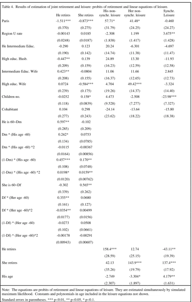
synchronous and non-synchronous leisure time of partners are given in Table 4. Results of estimation of the joint leisure model under the assumption that retirement decisions are exogenous (dropping the retirement equations) are provided in Table 5.
We find that the retirement probability increases significantly for individuals in a couple aged sixty and over, precisely by 0.17 percentage points for husband and by 0.18 for wives (see marginal estimates in Table 3a). The fact that partner reaches age sixty has no significant effect on individual retirement; however some of the partner’s cross-effects of age 60 with age polynomials are significant. The errors of the retirement equations are strongly positively correlated also disclosing positive interdependencies in partners’ preferences for retirement (see the correlations in Table 3b). As far as the other covariates go, higher education delays retirement as plausible, since higher education also delays entry into the labour market and, with that, also accumulation of pension rights. Partners residing in inner Paris retire
significantly later than the others, everything else equal, and this effect is especially strong for men: the retirement probability falls by 0.55 percentage points for men and by 0.33 for
women in a couple (see Table 3a). This could possibly reflect life-styles with Parisians having longer working life attitudes than individual residing in other provinces ore rural
neighbourhoods –notice that only 2 per cent of the sample of older couples resides in inner Paris (Table 1).
We conclude that own retirement increases significantly husband’s and wife’s disjoint leisure hours, defined as leisure that is not spent together (see Section 3.2 for definitions). In
particular, disjoint leisure increases by almost three hours a day upon own retirement –
precisely, 175 minutes for husbands and 167 minutes for wives (see Table 3). Looking at non-synchronized leisure, we find an increase of about two hours and a half per day upon
retirement –and, precisely, of 158 minutes for husbands and 144 minutes for wives (see Table 4). This is reasonable, since joint leisure is defined more narrowly than synchronized leisure and, thus, it follows naturally that “disjoint” leisure is larger than “non-synchronized” leisure. The effect of retirement of the husband on joint leisure hours is negative, while retirement of the wife has the expected positive sign. The effect of partners’ retirement on synchronous leisure is also strongly positive for the retirement of the wife and negative for the husband.
16
Her retirement increases joint leisure time by an hour and a half per day, while his retirement reduces it by about half an hour (see Table 3). These effects are a little larger when using a synchronous leisure measure as anticipated (see above discussion).
To look further into this asymmetry of responses of joint (synchronous) leisure to partners’ retirement we allow the effect of retirement on leisure hours to differ across week and
weekend days, exploiting the information on the day of collection of the time diary -recall that the diary was collected on the same day for all household members, which was chosen by the interviewer, and that we discarded atypical days (see Section 3 for more details). Then we find that his retirement reduces joint leisure on week days by about 30 minutes on average (though this effect is not significant statistically), while it increases joint leisure on a weekend day by 20 minutes (see Table 3d). Under this specification that enables us to capture different effects for different days of the week, each partner retirement has a significant negative and very tangible effect (and strongly significant) on the other partner’s disjoint leisure on week days (see Table 3c). In particular, his disjoint leisure increases by over two hours upon his retirement and by almost an extra hour on week days; to fall, however, on week days, by an hour and twenty minutes if she also retires (see Table 3c), which seems plausible as then they can spend more time together also on week days. As far as she is concerned, the effects are comparable: her disjoint leisure increases by over two hours when she retires and falls on week days by almost an hour if he also retires. However, notice that some of the cross-effects of partners retirement on own (disjoint) leisure time are positive, though not always
significant, suggesting that partner’s retirement increases own leisure at weekends. This seems also plausible as upon retirement more time is available, so that not only joint leisure increases if both partners are retired but also disjoint leisure does increase. The asymmetric results found for week days can then be understood in light of the fact that one partner is still at work.
Finally, it should be pointed out upfront, that because there are five week days and two weekend days in a week, the coefficients in Tables 3, 3c, and 3d, do not simply add up and to get an overall picture one has to look at Table 3 –where we assume that days where equally sampled by the data collectors (the day of the diary was indeed chosen by the interviewers to get a representative sample for each day of the week).
To sum up, the asymmetric effects we found may partly be due to the fact that husbands are on average older and thus are the first to retire. Later, we also added additional controls for
17
partners both retired, which however did not show up significant (see Table 7). An alternative explanation for these asymmetries is changes in partners’ valuation of leisure time spent together or separately upon retirement. And possibly also changes in partners’ negotiation power at retirement (see Section 2.1 for a discussion). Furthermore, as shown in Stancanelli and van Soest (2012) retirement increases dramatically the share of housework done by the husband and this may also contribute to explain the asymmetries we find in leisure time together.
Remarkably, results of estimation of the models without allowing for endogeneity of partners’ retirement decision (see Table 5) would lead us to conclude that retirement of either partner has a strongly significant and positive effect on joint leisure hours, thus hiding all of the asymmetries.
The correlations in the unobservables of the retirement equations of partners are strongly significant and positive (see Table 3a). On the contrary, the unobservables of the disjoint leisure equation of each partner are strongly negatively correlated with own retirement, while they are strongly positively correlated with each other. Furthermore, the unobservables of joint leisure time are strongly negatively correlated with the retirement equations of the wife and positively with that of the husband, suggesting some intriguing patterns that would reinforce the asymmetries observed. Therefore, endogenizing the retirement decision, retirement of the husband reduces joint leisure time of the partners but there are
unobservables driving his retirement decision and the leisure time together of partners that are positively correlated. The opposite is true for the wife: her retirement increases joint leisure time of the partners but there are unobservables driving her retirement decision and the leisure time together of partners that are negatively correlated. This may possibly be explained by the order of retirement, as husbands are on average older, as we already said. These
asymmetries in partners’ retirement decisions and leisure time together are also in line with the conclusions in Stancanelli and van Soest (2012) who found that while partner’s retirement increases own hour of home production, the cross-effect of the wife’s retirement on the husband’s home production hours is significantly negative. They also match well with the conclusions of the structural model of joint retirement of partners put forward by Gustman and Steinmeier (2009), who argue that in some cases individuals in a couple may decide to retire only if their partner does not retire and find, for the USA, that the increased labour force participation of women has actually contributed to lower husbands’ hours of market work.
18
As far as the other covariates go (back to Table 3), Parisian partners enjoy on average an extra hour of disjoint leisure per day, which is in line with the finding that they both retire later. The number of children reduces parents’ joint leisure hours by about 20 minutes per day. We also find that higher educated women enjoy an extra leisure hour on their own every day.
Furthermore, the local unemployment rate increases significantly her disjoint leisure but the effect is very small and equal to about three minutes a day (the sign is also positive for men but statistically insignificant).
Finally, we run a few robustness tests. Table 6 presents results of estimation using probits of retirement and tobit specifications for the hours of leisure equations. Using a tobit
specification implies that we assume that the zeros are censored observations: individuals reporting no joint leisure on the day of the diary would never carry out any leisure activity together, which is somewhat unlikely. Under a linear specification, we assume that the zeros are capturing infrequencies, i.e. the occurrence of zero today is random - as well as that of say, 2 hours and a half of joint leisure. Now, about 50 per cent of the observations in our sample do not carry any leisure activity together on the diary day. It seems unlikely to assume that they never carried out any leisure together. For this raison, our preferred specification for leisure time is linear (see Table 3). Under a tobit specification of the demands for leisure, our conclusions are not substantially affected – though the significance level of some variables changes slightly. In particular, the positive effect of his retirement on her disjoint leisure becomes statistically significant at the ten per cent level (while it is not significant in Table 3); the effect of her retirement on her disjoint leisure is now significant only at the ten per cent level (while it is strongly significant in Table 3) and his retirement has a weakly negative effect on leisure time together (while this effect is strongly significant in Table 3). Next, Table 7 presents results of estimation of the model as in Table 3 (our preferred specification) including additional controls for whether partners are both retired. This extra variable does not show up significant. Our main conclusions appear to be robust to these various alternative specifications.
6. Conclusions
In the scant literature on partners' joint retirement decisions one of the explanations for joint retirement is externalities in leisure. However, recent work also points to asymmetries in
19
partners’ retirement decisions. Earlier studies of joint retirement did not explicitly consider the extent to which partners spend their leisure time together.
In this study, we use diary data on leisure activities of older French partners to investigate the causal effect of individual and partner’s retirement on the time that the two partners devote to leisure time spent together. Our identification strategy exploits the fact that for many French workers, the earliest age at which a retirement pension can be drawn is age 60, which enables us to use a fuzzy regression discontinuity approach to identify the effect of both partners’ retirement on leisure.
The data for the analysis are drawn from the French time use survey 1998 which not only collects a diary for both partners on the same day but also asks questions as regards ‘with whom’ time was spent. Therefore, we can construct measures both of “synchronous” leisure of partners (requiring that the same leisure activity is carried out during the same time slot by the two partners) and of leisure time spent together (imposing additionally that both partners reported to have done the activity with family).
We estimate a five simultaneous equations system of partners’ retirement and leisure hours, including two equations for retirement and three for leisure hours -of each partner on his own and together. We find that the retirement probability increases significantly for spouses aged 60 and above, which supports our identification strategy. We conclude that although
retirement increases significantly the time each partner allocates to leisure activities, only retirement of the wife increases significantly leisure time together. The retirement of the husband has either no effect or a negative one, overall. Similar conclusions are drawn when analyzing synchronous leisure time of partners. These findings, which are robust to various sample selection and functional form sensitivity checks, can be partly understood in terms of differential effects of retirement on week and weekend days: his retirement increases joint leisure on weekend days but not so on week days. One possible explanation for this might be the order of retirement -as husbands are on average two years older than their wife. In line with this, we also find significantly negative cross-effects of each partner’s retirement on the other partner’s own (disjoint) leisure time on week days and positive cross-effects for his retirement on her leisure time at weekends.
Remarkably, results of estimation of the models without controlling for endogeneity of partners’ retirement decision would lead one to conclude that retirement of either partner has a strongly significant and positive effect on joint leisure time of partners, thus concealing all
20
of the asymmetries. Therefore, not controlling for selection into retirement would produce the results a priori anticipated in the literature; while controlling for selection into retirement elicits asymmetries in retirement and leisure choices of partners. These asymmetries are well in line with the conclusions of Gustman and Steinmeier (2009) who argue that partners do not always decide to retire together and actually find contrasting for the USA evidence that increased labour force participation of women may have lowered husbands’ hours of market work. Our findings also match those from a companion paper on retirement and house work (Stancanelli and Van Soest, 2012), where we concluded that while own retirement increases own house work, the wife’s retirement reduces the housework done by the husband,
suggesting that there is substitution in partners’ house work time.
In conclusion, partners with stronger preferences for spending leisure time together may retire earlier than others. However, retirement may change both their bargaining power and their preferences for leisure together, so that, in particular, leisure spent on their own may become more valuable when both partners are retired. It may also increase the share of housework done by the husband –who is often the first to retire- and thus free leisure time of the wife. This may contribute to generate asymmetries in leisure and retirement of partners rather than complementarities.
References
Mark Aguiar and Erik Hurst, 2007, Measuring Trends in Leisure: The Allocation of Time over Five Decades, The Quarterly Journal of Economics, MIT Press, 122(3), 969-1006. Battistin, Erich, Agar Brugiavini, Enrico Rettore and Guglielmo Weber (2009), The Retirement Consumption Puzzle: Evidence from a Regression Discontinuity Approach
American Economic Review, 99(5), 2209-2226.
Blanchet, Didier and Louis-Paul Pele (1997), Social Security and Retirement in France, NBER Working Paper No. 6214.
Bozio, Antoine (2004), “Does Increasing Contribution Length Lead to Higher Retirement Age? Evidence from the 1993 French Pension Reform”, mimeo.
Card, David, Carlos Dobkin and Nicole Maestas (2009), Does Medicare Save Lives?,
Quarterly Journal of Economics, 124(2), 597-636.
Card, David, Carlos Dobkin and Nicole Maestas (2004), The Impact of Nearly Universal Insurance Coverage on Health Care Utilization and Health: Evidence from Medicare, NBER Working Paper 10365.
21
Gustman, Alan and Thomas Steinmeier (2009), Integrating Retirement Models, NBER Working Paper 15607.
Gustman, Alan and Thomas Steinmeier (2000), Retirement in Dual-Career Families: A Structural Model, Journal of Labor Economics, 18, 503-545.
Hallberg, Daniel (2003), Synchronous Leisure, Jointness and Household Labor Supply,
Labour Economics, 10(2), 185-203.
Hamermesh, Daniel S. (2000), Togetherness: Spouses' Synchronous Leisure, and the Impact of Children, NBER Working Papers 7455.
Hamermesh, Daniel S. (2002), Timing, Togetherness and Time Windfalls, Journal of
Population Economics, 15(4), 601-623.
Hurd, Michael (1990), The Joint Retirement Decision of Husbands and Wives, in: Issues in
the Economics of Aging, David Wise (ed.), NBER, pp. 231-258.
Lundberg, S., R. Startz and S. Stillman (2003), The Retirement-Consumption Puzzle: A Marital Bargaining Approach, Journal of Public Economics, 87(5-6), 1199-1218.
Maurin, Eric and Aurelie Ouss (2009), "Sentence Reductions and Recidivism: Lessons from the Bastille Day Quasi Experiment," IZA Discussion Papers 3990.
Imbens, Guido and Thomas Lemieux (2007), Regression Discontinuity Design: a Guide to Practice, Journal of Econometrics, 142, 615-635.
Van der Klaauw, Wilbert (2008), Regression-Discontinuity Analysis: A Survey of Recent Developments in Economics, Labour, 22(2), 219-245.
Van der Klaauw, Wilbert (2002), Estimating the Effect of Financial Aid Offers on College Enrollment: A Regression-Discontinuity Approach, International Economic Review, 43(4), 1249-1287.
Lee, David S. and Thomas Lemieux (2010), Regression Discontinuity Designs in Economics,
Journal of Economic Literature, 48(2), 281-355.
Robinson, John and Geoffrey Godbey (1997), Time for Life: The Surprising Way Americans
Spend Their Time, University Park, The Pennsylvania State University Press.
Roodman, David (2009), Estimating Fully Observed Recursive Mixed-Process Models with CMP. Working Papers 168, Center for Global Development.
Roodman, David (2007), CMP: Stata Module to Implement Conditional (Recursive) Mixed Process Estimator. Statistical Software Components S456882, Boston College Department of Economics, revised 22 May 2009.
Sayer, Liana, Suzanne Bianchi and John Robinson (2001), Time Use Patterns of Older Americans, Report to NIA, University of Maryland.
22
Stancanelli, Elena and Arthur Van Soest (2012), Retirement and Home Production: A Regression Discontinuity approach, American Economic Review, Papers and Proceedings, May 2012, forthcoming.
Stancanelli, Elena and Leslie Stratton (2010), Her Time, His Time, or the Maid's Time: An Analysis of the Demand for Domestic Work, IZA DP 5253.
23
Table 1. Sample descriptives
Male partner Female partner
Mean standard deviation Mean standard deviation
Age (in years) 60.72 5.50 58.60 5.61
Age 60 or older,
dummy 0.57 0.49 0.43 0.47
Retired 0.64 0.48 0.67 0.47
Employed 0.36 0.48 0.32 0.47
Born in France 0.96 0.18 0.97 0.16
High School (12 years
schooling) 0.12 0.32 0.10 0.30
College and more 0.15 0.36 0.11 0.31
Bad health 0.03 0.18 0.05 0.23
Household characteristics
Mean standard deviation
Number of children at home 0.15 0.51 Cohabiting 0.04 0.19 Resides in Paris 0.02 0.15 Regional Unemployment rate 11.45 2.46
Weekend time diary 0.23 0.42
Observations 1043
24
Table 2. Participation rate and mean duration of market work and leisure
Male partner Female partner
Participation rate % Mean duration (st. dev.) Median duration Participation rate % Mean duration (st. dev.) Median duration Market work 29.82 137.83 (235.46) 0 21.67 86.04 (182.88) 0 Disjoint Leisure 94.92 234.41 (168.02) 210 89.84 164.32 (128.27) 140 Joint Leisure 68.07 86.11 (92.95) 60 68.07 86.11 (92.95) 60 Non-synchronous leisure 93.38 196.12 (152.20) 170 85.14 126.03 (110.34) 100 Synchronous leisure 81.69 124.40 (111.51) 100 81.69 124.40 (111.51) 100
27
Table 3. Results of estimation of joint retirement and leisure: probits of retirement and linear leisure equations He retires She retires His leisure Her leisure Joint Leisure Paris -1.631*** -0.897*** 72.88** 64.96** -21.68 (0.358) (0.282) (35.15) (28.12) (20.66) Region U rate -0.0173 0.0194 0.483 3.730** 1.208 (0.0246) (0.0190) (1.997) (1.639) (1.214) He Intermediate Educ. -0.219 0.0797 19.00 -9.040 -1.388 (0.190) (0.144) (15.94) (13.15) (9.750) High educ. Husb. -0.425** 0.103 23.76 9.964 -6.693 (0.211) (0.162) (17.70) (14.56) (10.68) Intermediate Educ. Wife 0.393* -0.0436 2.740 5.243 8.306 (0.209) (0.160) (17.75) (14.62) (10.82) High educ. Wife 0.0704 -0.539*** -1.974 50.98*** -5.588 (0.240) (0.179) (22.41) (16.98) (12.27) Children no. -0.00222 0.147* 0.807 -8.538 -17.94*** (0.124) (0.0847) (10.53) (8.457) (6.232) Cohabitant 0.189 0.267 -27.63 -19.76 -9.446 (0.282) (0.246) (25.55) (21.06) (15.62) He is 60=Dm 0.556** -0.147 (0.281) (0.215) Dm * (His age -60) 0.260* 0.114 (0.136) (0.0857) Dm * (His age -60) ^2 -0.00996 -0.00683 (0.0167) (0.00925) (1-Dm) * (His age -60) 0.457*** 0.165** (0.109) (0.0749) (1-Dm) * (His age -60) ^2 0.0188 0.0159** (0.0124) (0.00766) She is 60=Df -0.309 0.599** (0.343) (0.270) Df * (Her age -60) 0.359** 0.0283 (0.163) (0.131) Df * (Her age -60)^2 -0.0362** 0.00968 (0.0181) (0.0163) (1-Df) * (Her age -60) -0.0277 0.0694 (0.105) (0.0691) (1-Df) * (Her age -60)^2 -0.00239 -0.000961 (0.00982) (0.00632) He retires 175.3*** 26.84 -40.47** (33.51) (28.24) (16.29) She retires 24.91 167.5*** 107.7*** (57.44) (29.62) (15.60) His age -1.891 -2.836 2.721** (2.585) (2.131) (1.385)
His age squared 0.499** 0.0562 -0.139
(0.222) (0.183) (0.129)
Her age -2.956 -2.803* -1.216
(2.220) (1.464) (0.996)
Her age squared -0.263 0.0787 0.0185
(0.203) (0.165) (0.122)
28
Table 3a. Marginal estimates of Probits of retirement (from the model in Table 3).
He retires She retires
Paris -0.585*** -0.335*** (0.101) (0.109) Region U rate -0.005 0.006 (0.007) (0.006) He Intermediate Educ. -0.0069 0.024 (0.063) (0.043)
High educ. Husb. -0.139* 0.031
(0.075) (0.048)
Intermediate Educ. Wife 0.103** -0.014
(0.047) (0.051)
High educ. Wife 0.020 -.190**
(0.068) (0.068) Children no. -0.000 0.046* (0.037) (0.027) Cohabitant 0.052 0.076 (0.073) (0.063) He is 60=Dm 0.170* -.0046 (0.087) 0.066 Dm * (His age -60) 0.077* 0.036 (0.041) (0.027) Dm * (His age -60) ^2 -0.003 -0.002 (0.005) (0.003) (1-Dm) * (His age -60) 0.136*** 0.052** (0.033) (0.023) (1-Dm) * (His age -60) ^2 0.005 0.005** (0.004) (0.002) She is 60=Df -0.094 0.180** (0.104) (0.076) Df * (Her age -60) 0.107** 0.009 (0.047) (0.041) Df * (Her age -60)^2 -.0010** 0.003 (0.005) (0.005) (1-Df) * (Her age -60) -0.008 0.022 (0.031) (0.022) (1-Df) * (Her age -60)^2 -0.0007 -0.0003 (0.0029) -.002
Note: The equations are probits of retirement and linear equations of leisure. Standard errors in parentheses. *** p<0.01, ** p<0.05, * p<0.1.
29
Table 3b. Correlations of the errors of the equations of the model of retirement and leisure time
Her retirement His leisure Her leisure Joint leisure
His retirement 0.252*** -0.154 -0.164 0.523*** (0.0865) (0.124) (0.125) (0.119) Her retirement -0.145 -0.501*** -0.504*** (0.220) (0.145) (0.105) His leisure 0.368*** -0.204*** (0.0529) (0.0594) Her leisure -0.178*** (0.0491)
Results of estimation are reported in Table 3.
*** p<0.01, ** p<0.05, * p<0.1.
30
Table 3c. Results of estimation of joint retirement and leisure: probits of retirement and linear leisure equations
He retires She retires His leisure Her leisure Joint Leisure
Paris -1.648*** -0.884*** 69.28* 63.92** -20.14 (0.360) (0.282) (35.88) (28.01) (20.67) Region U rate -0.0176 0.0186 0.944 3.522** 1.141 (0.0246) (0.0190) (2.007) (1.630) (1.217) He Intermediate Educ. -0.230 0.0764 19.33 -8.170 -1.289 (0.191) (0.143) (15.89) (13.06) (9.766)
High educ. Husb. -0.425** 0.0952 26.29 7.681 -7.986
(0.210) (0.162) (17.86) (14.49) (10.71)
Intermediate Educ. Wife 0.397* -0.0442 2.835 3.687 8.069
(0.209) (0.164) (17.75) (14.53) (10.84)
High educ. Wife 0.0670 -0.515*** -8.688 50.52*** -4.990
(0.241) (0.180) (24.17) (17.08) (12.27) Children no. -0.00387 0.140* 0.535 -6.655 -17.80*** (0.124) (0.0848) (10.76) (8.448) (6.248) Cohabitant 0.195 0.264 -26.70 -20.28 -10.48 (0.281) (0.245) (25.50) (20.90) (15.65) He is 60=Dm 0.554** -0.142 (0.282) (0.215) Dm * (His age -60) 0.265* 0.119 (0.137) (0.0881) Dm * (His age -60) ^2 -0.0103 -0.00703 (0.0169) (0.00942) (1-Dm) * (His age -60) 0.462*** 0.170** (0.109) (0.0750) (1-Dm) * (His age -60) ^2 0.0196 0.0167** (0.0123) (0.00769) She is 60=Df -0.312 0.608** (0.344) (0.271) Df * (Her age -60) 0.354** 0.0218 (0.164) (0.135) Df * (Her age -60)^2 -0.0354* 0.00993 (0.0182) (0.0169) (1-Df) * (Her age -60) -0.0281 0.0740 (0.106) (0.0688) (1-Df) * (Her age -60)^2 -0.00242 -0.000376 (0.00982) (0.00634) He retires 131.8*** 68.35** -29.96 (39.06) (32.26) (18.76) She retires 63.07 139.4*** 119.6*** (77.17) (37.22) (18.04) He retires*week day 57.12** -55.38*** -14.41 (24.73) (19.26) (13.30)
She retires*week day -80.45*** 27.95 -10.96
(23.75) (18.60) (12.79)
Note: Standard errors in parentheses. *** p<0.01, ** p<0.05, * p<0. Constants and age polynomials of leisure eq. not shown.
31
Table 3d. Results of estimation of joint retirement and leisure: probits of retirement and linear leisure equations
He retires She retires His leisure Her leisure Joint Leisure
Paris -1.643*** -0.878*** 70.21** 64.64** -20.48 (0.360) (0.280) (34.91) (27.97) (20.66) Region U rate -0.0179 0.0186 0.613 3.578** 1.117 (0.0245) (0.0189) (1.990) (1.630) (1.216) He Intermediate Educ. -0.231 0.0778 19.35 -8.336 -1.265 (0.190) (0.143) (15.88) (13.07) (9.761)
High educ. Husb. -0.421** 0.102 25.08 7.419 -7.933
(0.210) (0.160) (17.67) (14.49) (10.71)
Intermediate Educ. Wife 0.399* -0.0509 2.192 4.121 7.960
(0.207) (0.160) (17.68) (14.54) (10.83)
High educ. Wife 0.0651 -0.520*** -5.554 50.77*** -5.049
(0.239) (0.179) (22.11) (16.83) (12.26) Children no. -0.00439 0.141* 1.959 -7.476 -17.49*** (0.125) (0.0846) (10.45) (8.405) (6.237) Cohabitant 0.192 0.266 -27.10 -20.51 -10.41 (0.281) (0.244) (25.46) (20.93) (15.64) He is 60=Dm 0.554** -0.136 (0.282) (0.213) Dm * (His age -60) 0.265* 0.113 (0.137) (0.0843) Dm * (His age -60) ^2 -0.0104 -0.00656 (0.0168) (0.00911) (1-Dm) * (His age -60) 0.461*** 0.168** (0.109) (0.0742) (1-Dm) * (His age -60) ^2 0.0196 0.0165** (0.0123) (0.00757) She is 60=Df -0.307 0.603** (0.345) (0.268) Df * (Her age -60) 0.353** 0.0251 (0.164) (0.132) Df * (Her age -60)^2 -0.0353* 0.00940 (0.0183) (0.0165) (1-Df) * (Her age -60) -0.0287 0.0732 (0.105) (0.0685) (1-Df) * (Her age -60)^2 -0.00243 -0.000548 (0.00979) (0.00628) He retires 175.5*** 15.91 -46.16*** (33.33) (27.95) (15.98) She retires 8.779 164.5*** 110.1*** (55.03) (28.53) (15.17) He retires*weekend -0.448 38.57*** 20.60** (18.54) (14.62) (10.32) She retires*weekend 25.32 -14.59 6.516 (25.53) (20.33) (14.46)
Note: Standard errors in parentheses. *** p<0.01, ** p<0.05, * p<0. Constants and age polynomials of leisure eq. not shown.
32
Table 4. Results of estimation of joint retirement and leisure: probits of retirement and linear equations of leisure.
He retires She retires
His non-synchr. leisure Her non-synchr. leisure Synchr. Leisure Paris -1.511*** -0.873*** 57.71* 41.48* -0.460 (0.370) (0.275) (31.79) (24.25) (24.27) Region U rate -0.00143 0.0185 -2.308 1.199 3.675** (0.0248) (0.0187) (1.838) (1.417) (1.428) He Intermediate Educ. -0.290 0.123 20.24 -6.301 -4.697 (0.190) (0.142) (14.74) (11.38) (11.47) High educ. Husb. -0.447** 0.139 24.89 13.30 -11.93 (0.209) (0.159) (16.23) (12.59) (12.58) Intermediate Educ. Wife 0.423** -0.0804 11.06 11.66 2.845
(0.208) (0.155) (16.37) (12.65) (12.73) High educ. Wife 0.0724 -0.584*** 4.704 49.42*** -3.324 (0.239) (0.175) (19.26) (14.37) (14.40) Children no. -0.0252 0.158* 4.473 -2.508 -23.98*** (0.118) (0.0839) (9.528) (7.277) (7.327) Cohabitant 0.104 0.298 -24.14 -13.64 -15.80 (0.277) (0.243) (23.62) (18.22) (18.38) He is 60=Dm 0.597** -0.102 (0.285) (0.209) Dm * (His age -60) 0.262* 0.0753 (0.134) (0.0785) Dm * (His age -60) ^2 -0.0115 -0.00367 (0.0164) (0.00856) (1-Dm) * (His age -60) 0.457*** 0.170** (0.108) (0.0748) (1-Dm) * (His age -60) ^2 0.0198* 0.0159** (0.0120) (0.00762) She is 60=Df -0.302 0.565** (0.339) (0.262) Df * (Her age -60) 0.355** 0.0680 (0.161) (0.127) Df * (Her age -60)^2 -0.0354** 0.00499 (0.0177) (0.0156) (1-Df) * (Her age -60) -0.0273 0.0508 (0.102) (0.0661) (1-Df) * (Her age -60)^2 -0.00178 -0.00291 (0.00943) (0.00607) He retires 158.4*** 12.74 -43.11** (28.59) (25.15) (19.39) She retires 42.13 143.9*** 137.4*** (35.26) (19.79) (17.92) His age -2.749 -3.304* 4.179** (2.307) (1.897) (1.631) Note: The equations are probits of retirement and linear equations of leisure. They are estimated simultaneously by simulated maximum likelihood. Constants and polynomials in age included in the leisure equations not shown.
33
Table 5. Results of estimation of joint leisure, assuming that retirement choices are exogenous
Leisure Time Together
Paris -21.28 (18.71) Region U rate 1.857* (1.113) He Intermediate Educ. 3.408 (8.951)
High educ. Husb. 5.138
(9.737)
Intermediate Educ. Wife 0.695
(9.951)
High educ. Wife -19.72*
(10.98) Children no. -14.38** (5.701) Cohabitant -5.244 (14.35) He retires 45.39*** (10.08) She retires 25.98*** (7.004)
Standard errors in parentheses. *** p<0.01, ** p<0.05, * p<0.1. Constant and age polynomials not shown.
34
Table 6. Results of estimation of joint retirement and leisure: probits of retirement and tobits of leisure
He retires She retires His leisure Her leisure Joint Leisure
Paris -1.701*** -0.876*** 55.30 59.73* -22.05 (0.368) (0.299) (36.62) (30.58) (29.63) Region U rate -0.0165 0.0231 1.104 4.395** 2.499 (0.0251) (0.0197) (2.111) (1.752) (1.671) He Intermediate Educ. -0.201 0.114 24.10 -5.741 0.0738 (0.192) (0.149) (16.85) (13.98) (13.48)
High educ. Husb. -0.430** 0.151 32.27* 15.11 -8.302
(0.215) (0.166) (18.84) (15.66) (14.87)
Intermediate Educ. Wife 0.347* -0.0264 -3.393 1.828 11.09
(0.210) (0.166) (18.76) (15.57) (14.95)
High educ. Wife -0.00523 -0.582*** -26.36 44.88** -12.70
(0.247) (0.181) (23.51) (20.13) (18.02) Children no. 0.00319 0.146* 7.142 -4.592 -26.12*** (0.127) (0.0857) (11.05) (9.340) (9.191) Cohabitant 0.205 0.243 -22.71 -18.34 -9.010 (0.287) (0.259) (27.03) (22.52) (21.47) He is 60=Dm 0.598** -0.146 (0.288) (0.245) Dm * (His age -60) 0.255* 0.130 (0.142) (0.0903) Dm * (His age -60) ^2 -0.00817 -0.00810 (0.0178) (0.0100) (1-Dm) * (His age -60) 0.474*** 0.197** (0.109) (0.0841) (1-Dm) * (His age -60) ^2 0.0207* 0.0199** (0.0123) (0.00835) She is 60=Df -0.386 0.780*** (0.355) (0.289) Df * (Her age -60) 0.391** -0.0222 (0.169) (0.143) Df * (Her age -60)^2 -0.0399** 0.0163 (0.0188) (0.0180) (1-Df) * (Her age -60) -0.0195 0.0301 (0.109) (0.0764) (1-Df) * (Her age -60)^2 -0.00215 -0.00328 (0.0101) (0.00694) He retires 207.9*** 54.48* -46.12* (36.01) (31.23) (24.48) She retires -80.71 102.1* 142.0*** (58.91) (56.81) (34.62)
Note: The equations are probits of retirement and tobits of leisure. They are estimated simultaneously by simulated maximum likelihood. Constants not shown.
35
Table 7. Results of estimation of joint retirement and leisure: probits of retirement and linear equations of leisure. Including additional controls for both partners’ retirement
He retires She retires His leisure Her leisure Joint Leisure
Paris -1.633*** -0.898*** 70.35** 63.89** -21.50 (0.358) (0.283) (35.36) (28.09) (20.68) Region U rate -0.0173 0.0192 0.508 3.739** 1.209 (0.0246) (0.0191) (1.997) (1.635) (1.215) He Intermediate Educ. -0.217 0.0800 18.05 -9.530 -1.231 (0.190) (0.144) (15.93) (13.12) (9.767)
High educ. Husb. -0.423** 0.104 20.78 8.472 -6.248
(0.211) (0.162) (17.82) (14.63) (10.76)
Intermediate Educ. Wife 0.390* -0.0411 3.905 5.841 8.114
(0.209) (0.161) (17.75) (14.60) (10.84)
High educ. Wife 0.0668 -0.540*** -0.449 51.88*** -5.949
(0.241) (0.180) (22.89) (17.14) (12.32) Children no. -0.00129 0.146* 0.814 -8.577 -17.90*** (0.125) (0.0849) (10.58) (8.452) (6.238) Cohabitant 0.189 0.265 -29.08 -20.54 -9.193 (0.282) (0.247) (25.54) (21.01) (15.65) He is 60=Dm 0.553** -0.155 (0.282) (0.217) Dm * (His age -60) 0.260* 0.120 (0.136) (0.0864) Dm * (His age -60) ^2 -0.00999 -0.00742 (0.0167) (0.00933) (1-Dm) * (His age -60) 0.457*** 0.168** (0.109) (0.0755) (1-Dm) * (His age -60) ^2 0.0189 0.0162** (0.0124) (0.00773) She is 60=Df -0.304 0.616** (0.344) (0.273) Df * (Her age -60) 0.360** 0.0218 (0.163) (0.132) Df * (Her age -60)^2 -0.0363** 0.0104 (0.0181) (0.0165) (1-Df) * (Her age -60) -0.0285 0.0687 (0.105) (0.0697) (1-Df) * (Her age -60)^2 -0.00244 -0.000880 (0.00984) (0.00637) He retires 179.8*** 29.40 -41.21** (33.89) (28.46) (16.37) She retires 20.39 165.9*** 107.7*** (62.45) (32.09) (15.65) Both retire -21.32 -10.68 3.027 (13.70) (10.96) (7.926)
Note: The equations are probits of retirement and linear equations of leisure. They are estimated simultaneously by simulated maximum likelihood. Constants not shown.