An Equilibrium Model of Health Insurance Provision and Wage
Determination
1
Matthew S. Dey
U.S. Bureau of Labor Statistics
Christopher J. Flinn
New York University
First Draft: April 2000
This Draft: December 2003
Keywords
: Health Insurance, Equilibrium Models, Wage Bargaining, Job Mobility
JEL
: D83, J32, J41
1This research was partially supported by grants from the Economic Research Initiative on the Uninsured
at the University of Michigan and the C.V. Starr Center for Applied Economics at New York University. We are grateful for comments received from participants in the “Econometrics of Strategy and Decision Making” conference held at the Cowles Foundation in May 2000, the annual meeting of the European Society for Population Economics held in Bonn in June 2000, the meetings of the Canadian Econometric Study Group held in October 2002, and seminar participants at Chicago, McGill, Ohio State, UCSD, Pompeu Fabra, CREST, UCLA, Georgetown, and Wisconsin. We have also received many valuable comments from Jaap Abbring, Jeffrey Campbell, Donna Gilleskie, Vijay Krishna, Jean-Marc Robin, and three anonymous referees. The views expressed here are ours and do not necessarily represent the views of the U.S. Department of Labor or the Bureau of Labor Statistics. We are responsible for all errors, omissions, and interpretations.
Abstract
We investigate the effect of employer-provided health insurance on job mobility rates and economic welfare using a search, matching, and bargaining framework. In our model, health insurance coverage decisions are made in a cooperative manner that recognizes the productivity effects of health insurance as well as its nonpecuniary value to the employee. The resulting equilibrium is one in which not all employment matches are covered by health insurance, wages at jobs providing health insurance are larger (in a stochastic sense) than those at jobs without health insurance, and workers at jobs with health insurance are less likely to leave those jobs, even after conditioning on the wage rate. We show that for inefficient mobility decisions to occur in our framework requires thatfirms be heterogeneous with respect to their costs of providing health insurance. We estimate the primitive paramters of the model using data from the SIPP 1996 panel and find that the empirical implications of the estimated model are in accord with both the data and anecdotal evidence. Heterogeneity in the distribution of firm costs of health insurance does lead to some inefficient (in the short-run) mobility decisions, but the vast majority of moves from job to job are associated with productivity improvements.
1
Introduction
Health insurance is most often received through one’s employer in the United States. According to U.S. Census Bureau statistics, almost 85 percent of Americans with private health insurance obtain their coverage in this manner. This strong connection between employment decisions and health insurance coverage has resulted in a substantial amount of research exploring the possible explanations for and impacts of this linkage. One branch of the literature has investigated the relationship between employer-provided health insurance and job mobility. In spite of a substantial amount of research on the issue, the relationship between health insurance coverage and mobility rates has not as yet been satisfactorily explained. Basing their arguments largely on anecdotal evidence, many proponents of health care reform claim that the present employment-based system causes some workers to remain in jobs they would “rather” leave since they are “locked in” to their source of health insurance. While it is true that individuals with employer-provided health insurance are less likely to change jobs than others (Mitchell, 1982; Cooper and Manheit, 1993), the claim that health insurance is the cause of this result has not been established. Madrian (1994) estimates that health insurance leads to a 25 percent reduction in worker mobility, while Holtz-Eakin (1994) finds no effect, even though they use an identical empirical methodology. Building on their approach, Buchmueller and Valletta (1996) and Anderson (1997) arrive at an estimate of the negative impact of health insurance on worker mobility that is slightly larger (in absolute value) than Madrian’s, while Kapur (1998) concludes there is no impact of health insurance on mobility. The most recent and only paper in this literature that attempts to explicitly model worker decisions, Gilleskie and Lutz (2002), finds that employment-based health insurance leads to no reduction in mobility for married males and a relatively small (10 percent) reduction in mobility for single males. Using statewide variation in continuation of coverage mandates, Gruber and Madrian (1994)find that an additional year of coverage significantly increases mobility, which they claim establishes that health insurance does indeed cause reductions in mobility. While this literature has extensively examined how the employment-based health insurance system affects mobility, the more pressing welfare implications have largely been ignored (Gruber and Madrian (1997) and Gruber and Hanratty (1995) are notable exceptions).
If health insurance coverage is strictly a nonpecuniary part of the compensation package offered by an employer, like a corner office or reserved parking space, the theory of compensating diff er-entials would predict a negative relationship between the cost (or provision) of health insurance and wages conditional on the value of the employment match. Somewhat surprisingly (from this perspective), Monheit et al. (1985) estimate a positive relationship between the two. Subsequent research has attempted to exploit potentially exogenous variation from a variety of sources in order to accurately identify the “effect” of health insurance on wages. Gruber (1994) uses statewide variation in mandated maternity benefits, Gruber and Krueger (1990) employ industry and state variation in the cost of worker’s compensation insurance, and Eberts and Stone (1985) rely on school district variation in health insurance costs to estimate the manner in which wages are affected. All three conclude that most (more than 80 percent) of the cost of the benefit is reflected in lower wages. In addition, Miller (1995) estimates significant wage decreases for individuals moving from a job without insurance to a job with insurance. Hence, the research that examines to what extent health insurance costs are passed on to employeesfinds that a majority of the costs are borne by employees in the form of lower wages.
These results from the two branches of the literature seem inconsistent on the face of it. If individuals are bearing the cost of the health insurance being provided to them by their employer,
why are they apparently less likely to leave these jobs? In addition, the absence of a conceptual framework that is consistent with many of the empirical findings on “job lock” and the indirect costs of health insurance to workers means that few policy implications can be drawn from the empirical results that have been obtained.
In this paper we attempt to provide such a framework by developing and estimating an equilib-rium model of employer-provided health insurance and wage determination. The model is based on a continuous-time stationary search model in which unemployed and employed agents stochastically uncover employment opportunities characterized in terms of idiosyncratic match values. Firms and searchers then engage in Nash bargaining to divide the surpluses from each potential employment match. In contrast to traditional matching-bargaining models (e.g., Flinn and Heckman, 1982; Diamond, 1982; and Pissarides, 1985), we allow employee “compensation” to vary over both wages and health insurance coverage. In our framework, health insurance has two potential welfare im-pacts on the worker-firm pair. First, by inducing the employee to utilize health care services more frequently it increases his productivity in the sense of reducing the frequency of negative health outcomes that lead to the termination of the match. Due to search frictions, the preservation of an acceptable match provides a benefit to both the employer and the employee. Second, at least some individuals may exhibit a “private” demand for health insurance. We view this demand as mainly arising from the existence of uncovered dependents in the employee’s household.
The main novelty in our modeling framework is our view of health insurance as a productive factor in an employment match, in addition to any direct utility-augmenting effects it may have. As a result, the level of health insurance coverage is optimally chosen given the value of the produc-tivity match and idiosyncratic characteristics of the worker and firm. The productivity-enhancing nature of health insurance is modeled as follows. Since an employment contract may terminate due to the poor health of the employee, we view health insurance coverage as reducing the rate of “exogenous” terminations from this source. There is some support for our assumption in the empirical literature. Levy and Meltzer (2001) provide a very thorough survey of empirical research examining the relationship between health insurance coverage and health outcomes. With special reference to results from large-scale quasi-experimental studies and the Rand randomized exper-iment, the authors conclude that there exists solid evidence to “suggest that policies to expand insurance can also promote health.” Since we find overwhelming support for our assumption in the course of estimating the model,1 our results could be taken as adding further (albeit indirect) support to the proposition that health insurance improves health.
Beginning from this premise, we are able to derive a number of implications from the model that coincide with both anecdotal and empirical evidence. Most basically, the model implies that: (1) not all jobs will provide health insurance, (2) workers “pay” for health insurance in the form of lower wages, and (3) jobs with health insurance coverage tend to last longer than those without (both unconditionally and conditionally on wage rates).
In order to explicitly investigate the “job lock” phenomenon, it is necessary for us to allow for on-the-job search with resulting job-to-job transitions. This necessitates that we model the process of negotiation between a worker and two potential employers which we are able to accomplish after making some stringent assumptions regarding the information sets of the agents involved in the bargaining game. This is the first attempt to estimate such a model in a Nash bargaining context, though using French worker-firm matched data Postel-Vinay and Robin (2000) estimate 1We do not impose the theoretical restriction when the model is estimated, yet find that the estimated rate of
an equilibrium assignment model that includes renegotiation.2 They assume thatfirms appropriate all of the rents from the match, which is a limiting case of the Nash bargaining model we employ.
Estimates of the primitive parameters characterizing the model using data from the 1996 panel of the Survey of Income and Program Participation (SIPP) tend to support our model specification. In particular, wefind that the rate of “involuntary” separations from jobs without health insurance is about 8 times greater than at jobs with health insurance. We find broad conformity with the implications of the model on a number of other dimensions as well. The raw data suggest that jobs providing health insurance are substantially longer than those that do not provide it, though due to substantial amounts of right-censoring of spell lengths the precise magnitude of the difference is difficult to determine. Model estimates imply that the ratio is on the order of 6. The model also does a reasonably good job of fitting the observed conditional wage distributions (by health insurance status) and the unconditional distribution of wages.
We are also able to look at the claim that nonuniversally-provided health insurance leads to inefficient mobility decisions. We demonstrate that within our model all mobility decisions are efficient in a generalized sense. We allow for heterogeneity in the population of firms with respect to the cost of providing and health insurance and within the population of searchers with respect to the “private” valuation of health insurance. While time-invariant searcher heterogeneity cannot lead to inefficient turnover decisions, time invariantfirm heterogeneity can, at least in one specific sense. A worker who faces the choice between twofirms at a point in time with two known match values θ and θ0 may choose to work at the lower match value firm if that firm offers lower costs of health insurance than does the other. While the match chosen will always be the one providing higher total surplus to the worker-firm pair, the fact that a lower match value is chosen may be taken to represent a form of inefficiency - at least in comparison with a world in which all potential matches face the same cost of providing coverage. Given our estimates of the health insurance cost distribution within the population of employers, even this limited form of “inefficiency” is found to be virtually nonexistent. Based on our model specification and estimates, we find little indication that the current employer-based health insurance system causes individuals to pass up productivity-improving job opportunities.
Due to data limitations and also for reasons of tractability we have decided to only consider whether health insurance is provided or not and additionally assume that the employer’s direct cost of purchasing health insurance is exogenously determined. In reality the provision of health insur-ance involves many complicating features, both at the plan level and with respect to the costs that employers face. In particular, plans may cover both the worker (who supplies the productivity) and his family. Implicit in our empirical work is the assumption that health insurance coverage is ex-tended to other family members. Moreover, for various reasons insurance contracts usually involve cost-sharing and risk-sharing features (e.g., deductibles, co-payment rates, and annual maximums, etc.). While these features are undoubtedly important factors in the decision-making process, the data requirements necessary to consider these elements are well beyond the scope of any currently available data set. In a similar vein, employers can either purchase coverage from an insurance provider with whom they may be able to bargain over the premiums based on employee demo-graphics or self-insure. By allowing firm-level heterogeneity in the cost of health insurance provi-sion we are capturing (in an admittedly indirect manner) some of these features. Lastly, although perhaps most importantly, our model ignores the relative tax advantage of compensation in the 2The recent paper by Cahuc et (2003) uses a similar bargaining structure to the one employed in this paper, though
form of health insurance benefits. While the favored tax status of health insurance affects the wage and health insurance distribution, we argue that this cannot be the entire explanation for the role employers play in the provision of health insurance in the United States and the inclusion of tax parameters will not change the qualitative features of our model.
The remainder of the paper is structured as follows. In Section 2 we develop our search-theoretic model of the labor market with matching and bargaining which produces an equilibrium distribution of wages and health insurance status. Section 3 contains a discussion of the data used to estimate the equilibrium model, while Section 4 develops the econometric methodology. Section 5 presents the estimates of the primitive parameters and the implications of estimates for observable duration and wage distributions. We also develop formal measures of the extent of “inefficient” turnover, and use our estimates to compute them. In Section 6 we offer some concluding remarks.
2
A Model of Health Insurance Provision and Wage
Determina-tion
In this section we describe the behavioral model of labor market search with matching and bar-gaining. The model is formulated in continuous time and assumes stationarity of the labor market environment. We begin by laying out the structure of the most general model we estimate and then proceed to characterize some important properties of the equilibrium. We attempt to provide some intuition regarding empirical implications of the model through graphical illustrations of equilib-rium outcomes in the specification that ignores heterogeneity on the supply and demand sides of the market.
The key premise of the model is that health insurance has a positive impact on the productivity of the match. As is standard in most search-matching-bargaining frameworks, the instantaneous value of a worker-firm pairing is determined by a draw (upon meeting) from a nondegenerate distri-butionG(θ). This match value persists throughout the duration of the employment relationship as long as the individual remains “healthy.” A negative health shock while employed at match value
θ reduces the value of the match to 0 and results in what we will consider to be an exogenous dissolution of the employment relationship.3 Thus an adverse health shock is considered to be one, potentially important, source of job terminations into unemployment. To keep the model tractable we have assumed that a negative health shock on one job does not affect the labor market environ-ment of the individual after that job is terminated. Thus one should think of these health shocks as being largely employer- or job task-specific.
The role of health insurance in reducing the rate of separations into unemployment is presumed to result from covered employees more intensively utilizing medical services than non-covered em-ployees. As a result, the rate of separations due to an inability to perform the job task associated with the match θ will be lower among covered employees. If all other reasons for leaving a job and entering the unemployed state are independent of health insurance status, the wage, and the match value, thenη1< η0, whereηdis theflow rate from employment into unemployment for those in health insurance status d, with d = 1 for those with employer-provided health insurance and
d = 0 for those who are uncovered. In this manner the purchase of health insurance can extend the expected life of the match for any given match value θ through it’s “direct,” but stochastic, 3It is not strictly necessary that the value of the match be reduced to0,since any new value ofθthat would make
unemployment more attractive than continued employment at thefirm would do. The value0serves as a convenient normalization.
impact on health status. We will also consider other indirect effects of health insurance on match longevity that operate through a sorting mechanism.
Individuals are assumed to possess an instantaneous (indirect) utility function given by
uξ(w, d) =w+ξd,
where ξ ≥ 0. Individuals of type ξ = 0 will then behave as classic expected wealth maximizers and exhibit only a “derived demand” for health insurance as a productive factor in an employment relationship. Those individuals with ξ >0 have some “private” demand for health insurance and maximize a slightly different objective function. We assume that the population distribution of preference types is given byH(ξ).
The heterogeneity on the demand side of the market relates to the cost to a firm of providing health insurance coverage to any one of its employees. While modeling the cost of providing such coverage is an interesting issue in itself, here we simply assume that these costs are exogenously determined. The premium paid by a firm is given by φ where φ ∈ Φ ⊆ R+. We denote the
population distribution offirm types by F(φ).
Given the nature of the data available to us (from the supply side of the market), firms are treated as relatively passive agents throughout. In particular, we assume that the only factor of production is labor, and that the total output of the firm is simply the sum of the productivity levels of all of its employees. Then if the firm “passes” on the applicant — that is, does not make an employment offer — its “disagreement” outcome is 0 [it earns no revenue but makes no wage payment]. With the additional assumption that there are no fixed costs of employment to firms, the implication is that employment contracts are negotiated between workers and firms on an individualistic basis, that is, without reference to the composition of thefirm’s current workforce.
All individuals begin their lives in the nonemployment state, and we assume that it is optimal for them to search. The instantaneous utility flow in the nonemployment state is b, which can be positive or negative. When an unemployed searcher and a firm meet, which happens at rate
λn, the productive value of the match θ is immediately observed by both the applicant and the firm as are the firm and searcher types, φ and ξ, respectively. After both parties have been fully informed, a division of the match value is proposed using a Nash bargaining framework. If both parties realize a positive surplus the match is formed, and if not the searcher continues looking for an acceptable match. LetVξN denote the value of unemployed search to a searcher of type ξ, and denote by Qξ(θ, φ) the value of the match if the searcher receives all of the surplus. Then since
the disagreement value of the firm is 0, all matches with Qξ(θ, φ) ≥ VξN will be accepted by an
unemployed searcher of typeξand a typeφfirm.4 Let the value of an employment contact between a type ξ worker and a type φemployer with match value θ to the employee be VξE(w, d;θ, φ) and let the value of the same match to the firm be given by VξF(w, d;θ, φ). Then given an acceptable match, the wage and health insurance status of the employment contract are determined by the solution to the Nash bargaining game
( ˆwξ,dˆξ)(θ, φ, VξN) = arg maxw,d Ξξ(w, d;θ, φ, VξN). (1)
The Nash bargaining objective function is given by
Ξξ(w, d;θ, φ, VξN) = (VξE(w, d;θ, φ)−VξN)αVξF(w, d;θ, φ)1−α (2)
4
whereα∈(0,1)is the bargaining power of the individual.
Employed agents meet new potential employers at rate λe. To keep the model tractable we
assume that there is full information among all parties as to the characteristics associated with the current match(θ, φ)and the potential match(θ0, φ0), as well as the worker’s typeξ. This means that each firm knows the match value of the individual at the otherfirm with which it is competing for the worker’s services as well as thatfirm’s type. While these are strong informational assumptions, they are relatively inconsequential for the empirical analysis conducted below given the nature of the data available to us.
We now consider the rent division problem facing a currently employed agent who encounters a new potential employer. Assume that a currently employed typeξ individual faces two potential employers with characteristics, (θ, φ) and (θ0, φ0), where Qξ(θ0, φ0) ≥ Qξ(θ, φ) ≥ VξN. Under our
bidding mechanism, the individual will end up accepting the match at the type φ0 employer after the “last” offer by the type φfirm. The idea is that the type φ0 employer can match any feasible offer (i.e., any(w, d)such thatVξF(w, d;θ, φ)≥0) made by the typeφfirm and will therefore “win” the the worker’s services. The value of the offer of the dominatedfirm serves as the threat point of the employee in the Nash bargaining problem faced by the employee with the winningfirm. When this is the case, the Nash bargaining objective function is given by
Ξξ(w, d;θ0, φ0, θ, φ) = (VξE(w, d;θ0, φ0)−Qξ(θ, φ))αVξF(w, d;θ0, φ0)1−α (3) and the new equilibrium wage and health insurance pair will be given by
( ˆwξ,dˆξ)(θ0, φ0, θ, φ) = arg max
w,d Ξξ(w, d;θ
0, φ0, θ, φ). (4)
The firm’s value of the current employment contract is defined as:
VξF(w, d;θ, φ) = (1 +ρε)−1{(θ−w−dφ)ε+ηdε×0 (5) +λeε Z Φ Z ¯θ ξ(θ,φ,φ)˜ ˆ θξ(w,d,φ)˜ ˆ VξF(θ, φ,˜θ,φ)dG(˜˜ θ)dF(˜φ) +λeε Z Φ G(ˆθξ(w, d,φ))dF˜ (˜φ)× VξF(w, d;θ, φ) +λeε Z Φ ˜ G(¯θξ(θ, φ,φ))dF˜ (˜φ)×0 +(1−λeε−ηdε)VξF(w, d;θ, φ) +o(ε)},
where VˆξF(θ, φ,˜θ,φ) =˜ VξF( ˆwξ(θ, φ,˜θ,φ),˜ dξ(θ, φ,ˆ ˜θ,φ);˜ θ, φ) represents the equilibrium value to a typeφfirm of the productive matchθwhen the typeξ worker’s next best option has characteristics
(˜θ,φ)˜ . The functionˆθξ(w, d,φ)˜ is defined as the maximum value of ˜θfor which the contract(w, d)
would leave a typeφ˜ firm with no profit given that the individual is typeξ. This value is implicitly defined by the equation
VξF(w, d; ˆθξ(w, d,φ),˜ φ) = 0.˜
Any encounter with a potential type φ˜ firm in which the match value is less than ˆθξ(w, d,φ)˜ will
not be reported by the employee; any new contact with a match value greater than ˆθξ(w, d,φ)˜ will
be reported to the current firm and will result in either a renegotiation of the current contract or a separation. When the new potential employer can match any offer extended by the current firm
such that Qξ(˜θ,φ)˜ > Qξ(θ, φ), a separation will occur. That is, any new match˜θ >¯θξ(θ, φ,φ)˜ will
induce the worker to quit where the critical match is implicitly defined by
Qξ(¯θξ(θ, φ,φ),˜ ˜φ) =Qξ(θ, φ).
After rearranging terms and taking limits, we have
VξF(w, d;θ, φ) = [ρ+ηd+λe Z Φ ˜ G(ˆθξ(w, d,φ))dF˜ (˜φ)]−1 (6) ×{θ−w−dφ +λe Z Φ Z ¯θξ(θ,φ,φ)˜ ˆ θξ(w,d,φ)˜ ˆ VξF(θ, φ,˜θ,φ)dG(˜˜ θ)dF(˜φ)}.
For the employee, the value of employment at a current match (θ, φ) and wage and health insurance provision status(w, d)is given by
VξE(w, d;θ, φ) = (1 +ρε)−1{(w+ξd)ε+ηdεVξN (7) +λeε Z Φ Z ¯θ ξ(θ,φ,φ)˜ ˆ θξ(w,d,φ)˜ ˆ VξE(θ, φ,˜θ,φ)dG(˜˜ θ)dF(˜φ) +λeε Z Φ Z ¯ θξ(θ,φ,˜φ) ˆ VξE(˜θ,φ, θ, φ)dG(˜˜ θ)dF(˜φ) +λeε Z Φ G(ˆθξ(w, d,φ))dF˜ (˜φ)× VξF(w, d;θ, φ) +(1−λeε−ηdε)VξE(w, d;θ, φ) +o(ε)}
where VˆξE(θ, φ,˜θ,φ) =˜ VξE( ˆwξ(θ, φ,˜θ,˜φ),dξ(θ, φ,ˆ ˜θ,˜φ);θ, φ) represents the equilibrium value to a type ξ worker employed at a match with characteristics (θ, φ) when his next best option is defined by (˜θ,φ)˜ . Note that when an employee encounters a firm with a new match value lower than his current one but sufficiently great that it can be used to increase his share of the match surplus (i.e., a new draw ˜θ such that¯θξ(θ, φ,φ)˜ >˜θ > ˆθ(w, d,˜φ)), his new value of employment at the current firm becomes VξE( ˆwξ(θ, φ,˜θ,˜φ),dˆξ(θ, φ,˜θ,˜φ);θ, φ).
The receipt of outside offers during an employment match provides a rationale for wage growth on the job, as well as allowing for the possibility for a change in health insurance coverage. In fact, while the bargaining power parameterαis often the focus of attention when examining the labor’s share offirm revenues, competition between firms for workers can result in a very high labor share even in the presence of low bargain power. This point is clearly made in the empirical results of Postel-Vinay and Robin (2002), where the bargaining power of searchers is assumed to be zero, and in the empirical results presented below. In both cases, substantial amounts of wage growth are indicated with small or no bargaining power as long as employers are forced to bid against each other for a worker’s services sufficiently often.
In addition, when the potential surplus to the worker at the newly-contactedfirm exceeds that of the current firm (i.e., a new draw ˜θ such that ˜θ > ¯θξ(θ, φ,φ)˜ ), mobility results. The value of
employment at the new firm is given by VξE( ˆwξ(˜θ,φ, θ, φ),˜ dˆξ(˜θ,φ, θ, φ); ˜˜ θ,φ)˜ — that is, the match
value at the currentfirm becomes the determinant of the “threat point” faced by the newfirm and plays a role in the determination of the new wage. Finally, when the match value at the newfirm is
less thanˆθξ(w, d,φ)˜ , the contact is not reported to the currentfirm since it would not result in any
improvement in the current contract. Because of this selective reporting, the value of employment contracts must be monotonically increasing both within and across consecutive job spells. Declines can only be observed following a transition into the unemployment state.
After rearranging terms and taking limits, we have
VξE(w, d;θ, φ) = [ρ+ηd+λe Z Φ ˜ G(ˆθξ(w, d,φ))dF˜ (˜φ)]−1 (8) ×{w+ξd+ηdVξN +λe Z Φ Z ¯θ ξ(θ,φ,φ)˜ ˆθξ(w,d,˜φ) ˆ VξE(θ, φ,˜θ,φ)dG(˜˜ θ)dF(˜φ) +λe Z Φ Z ¯θξ(θ,φ,˜φ) ˆ VξE(˜θ,φ, θ, φ)dG(˜˜ θ)dF(˜φ)}.
The model is closed after specifying the value of nonemployment,VξN, and the total surplus of the match,Qξ(θ, φ). Passing directly to the steady state representation of VξN, we have
VξN = [ρ+λnG(θ˜ ∗ξ)]−1 (9) ×{b+λn Z Φ Z θ∗ ξ ˆ VξE(˜θ,φ, V˜ ξN)dG(˜θ)dF(˜φ)}
where θ∗ξ is the critical match value associated with the decision to initiate an employment con-tract for a typeξindividual andVˆξE(˜θ,φ, V˜ ξN) =VξE( ˆwξ(˜θ,φ, V˜ ξN),dˆξ(˜θ,φ, V˜ ξN); ˜θ,φ)˜ represents the
equilibrium value to a typeξ worker employed at a match with characteristics(˜θ,φ)˜ when coming out of the nonemployment state.5
The total surplus of the match is given by
Qξ(θ, φ) =VξE( ˆwξ(θ, φ, θ, φ),dˆξ(θ, φ, θ, φ);θ, φ),
where
( ˆwξ,dˆξ)(θ, φ, θ, φ) = ( ˆwξ,dˆξ)(θ, φ).
When the worker receives the entire surplus of the match the equilibrium wage function is par-ticularly simple to derive. Setting VξF(w, d;θ, φ) = 0 and recognizing that there is no room for renegotiation, we have θ−w−dφ= 0⇒wξ(θ, φ) =ˆ θ−φdξ(θ, φ).ˆ (10) Then Qξ(θ, φ) = [ρ+η( ˆdξ(θ, φ)) +λe Z Φ ˜ G(¯θξ(θ, φ,φ))dF˜ (˜φ)]−1 (11) ×{θ−(φ−ξ) ˆdξ(θ, φ) +η( ˆdξ(θ, φ))VξN +λe Z Φ Z ¯ θξ(θ,φ,˜φ) ˆ VξE(˜θ,˜φ, θ, φ)dG(˜θ)dF(˜φ)}. 5
We are implicitly assuming that for every pair of worker-firm types(ξ, φ), there exist some employment contracts that do not result in the purchase of health insurance coverage. Without this assumption, the critical match would depend on the type offirm the individual meets out of nonemployment.
where we have used the fact thatˆθξ( ˆwξ(θ, φ),dˆξ(θ, φ),φ) = ¯˜ θξ(θ, φ,φ)˜ .
We can now characterize the wage and health insurance decisions with the following set of results.
Proposition 1 Let Qξ(θ0, φ0)> Qξ(θ, φ) where (θ, φ) represent the characteristics of the next best option available to a type ξ employee at the time a bargain is made. The decision to acquire health insurance is only a function of (θ0, φ0, ξ).
Proof: See Appendix A.
The decision to acquire health insurance is an efficient one in the sense that it only depends on characteristics of the current match. The driving force behind this result is the manner in which the “private” demand for health insurance enters the individual’s contemporaneous utility function. It enters linearly, and essentially combines with the firm’s cost characteristic φ to produce a net health insurance cost ofφ−ξ. The linearity implies the health insurance decision is never revisited as a result of a new division of the match surplus. Thus the health insurance decision is made solely to maximize the total surplus from the match and is efficient given the cost of health insurance
φ−ξ.
Proposition 2 Assume there exist employment contracts between a type φ employer and type ξ employee that do not result in the purchase of health insurance. The decision to initiate an em-ployment contract can be characterized by a unique critical matchθ∗ξ. Furthermore, when a type ξ individual works for a type φ employer the decision to purchase health insurance coverage can be characterized by a unique critical match, θ∗∗ξ (φ).
Proof: See Appendix B.
This result simply establishes the existence of critical value strategies for the bargaining pair. The assumption that there exists some acceptable match values that do not result in health insur-ance coverage for all pairs(φ, ξ)simplifies the characterization of labor market equilibrium and the computational task we face. There would be no conceptual difficulty in relaxing this assumption.
When there existsfirm heterogeneity “inefficient” mobility decisions will occur, in general. By an “inefficient” mobility decision we mean that when confronted with a choice between θ and θ0,
where θ0 > θ, the individual (optimally) opts for θ.6 The reason for this is that, from a type ξ
searcher’s perspective, an employment contact now is characterized by the two values(θ, φ).Since the value of the potential match is a function of both, when confronted with a choice between
(θ0, φ0) and (θ, φ),the decision rule will not generally be only a function of θ0 and θ.
The potential for inefficiency, by which we really only mean that(θ, θ0)is not a sufficient statistic for the mobility decision, only arises in certain cases. Clearly, when two potential matches exist with the same type of firm7 the individual will always choose the one with the highest value ofθ, or
Qξ(θ0, φ)> Qξ(θ, φ)⇔θ0> θ, ∀φ.
Thus inefficient mobility decisions can never occur when the searcher’s choice is between twofirms of the same type. In this case the values(θ, θ0)are sufficient for characterizing the mobility decision.
6
By inefficiency here we mean that the highest match value is not always taken. In the context of this model it is doubtful that this is the correct criterion to use as is discussed more fully below.
7
For the likelihood that two firms of the same type would be bidding against each other to be nonzero it is necessary that the distribution offirm types to have mass points. This is the case in the econometric specification we employ.
Now consider the case in which the agent faces a choice between firms of different cost types. Say that his current match is at a lower costfirm than the potential match,φ < φ0. Since the value of employment is non-increasing in the cost of health insurance, the match values at the higher cost
firm will have to be at least as large as the match value at the lower costfirm for mobility to occur. If the individual would not purchase health insurance at eitherfirm then the types of thefirms are irrelevant. In such a case, the match values at the two firms are (conditionally) sufficient for the mobility decision and no inefficient mobility can result (and in this case the value of working at either firm at the same match value is equal). Now consider the case in which the match value at the lower costfirm results in the purchase of health insurance. Let the current employment match be characterized by(θ, φ)and the potential employment match be characterized by(θ0, φ0). If both matches would result in health insurance being purchased, the agent must be compensated for the increased cost of health insurance. In this case, there exists a critical value ¯θξ(θ, φ, φ0) > θ such
thatQξ(¯θξ(θ, φ, φ0), φ0) =Qξ(θ, φ) for which the agent will be indifferent between the twofirms. It is also possible that there could exist a draw of θ0 at the higher cost firm that resulted in mobility but did not result in health insurance. In such an instance it is also necessary to compensate the individual for the loss of health insurance (whatever the value of ξ), and this also implies that the critical match value¯θξ(θ, φ, φ0)> θ. Thus there will always be a “wedge” between the critical
match value required for mobility to a higher costfirm and the current match valueθ at the lower costfirm whenever the individual has health insurance. This wedge generates something analogous to what is known as “job lock” in the empirical literature that studies mobility, wage, and health insurance outcomes. This occurs when an individual passes on a higher match at a higher costfirm to keep a lower match at a lower costfirm.
The other possibility for inefficient mobility decisions occurs when the agent is currently em-ployed at a higher costfirm(θ, φ)and meets a low costfirm(θ0, φ0)whereφ0 < φ. If the agent would have no health insurance at eitherfirm, then the mobility decision is made on the basis of theθand
θ0 draws exclusively and is consistent with efficiency. When the current match at the higher cost
firm provides health insurance, then there once again exists a wedge between the current value of the match at the higher costfirm and that required for mobility to the lower cost firm. As before, define ¯θξ(θ, φ, φ0) such that Qξ(¯θξ(θ, φ, φ0), φ0) = Qξ(θ, φ) and note that ¯θξ(θ, φ, φ0) < θ. When
the match at the higher cost firm does not result in health insurance, there still exists a wedge when the match at the lower cost firm does. When an individual leaves a higher cost firm match for a lower-valued match at a lower cost firm we may term this as “job push” as in the empirical literature on the subject. Clearly “job lock” and “job push” are two sides of the same coin in our framework, with the distinction between the two solely arising from whether the current match is with a lower cost or higher costfirm.
The model is sufficiently complex that comparative statics results are not readily available. In light of this we will only graphically display some of the implications of the model. Due to the relatively complicated renegotiation process it is difficult to solve for the steady state wage distribution, which is the cross-sectional distribution that would be observed after the labor market had been running for a sufficiently long period of time. The distributions that are plotted are all based on some of the model estimates obtained below; the specific model utilized for these illustrative purposes is the simplest one in which there is no heterogeneity on either side of the market and there is symmetric bargaining, i.e., α= 0.5.
Figure 1 plots the estimated probability density function of job matches in the population, which is assumed to belong to the lognormal family. The lower dotted line represents the critical match
value for leaving unemployment, θ∗, which is estimated to be approximately 7.76. The dotted line to the right represents θ∗∗, which is the critical match value for the match to provide health insurance coverage (its estimated value is 13.95). The likelihood that an unemployed searcher who encounters a potential employer will accept a job is the measure of the area to the right ofθ∗. The probability that an unemployed searcher accepts a job that doesn’t provide health insurance is then given by the probability mass in the area between the two critical values divided by the probability of finding an acceptable match, which in this case is 0.43.
The wage densities (associated with the first job after leaving unemployment) conditional on health insurance status are displayed in Figure 2.a. We can clearly discern the area of overlap between these two densities. Since both of these p.d.f.s are derived from slightly different mappings of the same p.d.f. g(θ), it is not surprising that they share general features in terms of shape. Note that the wage density conditional on not having health insurance is always defined on afinite interval[w(0), w(0)), while the range of wages conditional on having health insurance is unbounded as long as the matching distribution Ghas unbounded support. These general characteristics also characterize the conditional steady state wage distributions.
In Figure 2.b we plot the marginal wage density associated with thefirst wage observed following unemployment. The interval of overlap in the wage distribution adds a “bulge” to a density that otherwise resembles the parent lognormal density. Recall that wages in the interval of the bulge are the only ones that can either be associated with health insurance or not. Wages in the right tail are always associated with jobs that provide health insurance while those to the left of the bulge are associated with jobs that do not provide health insurance.
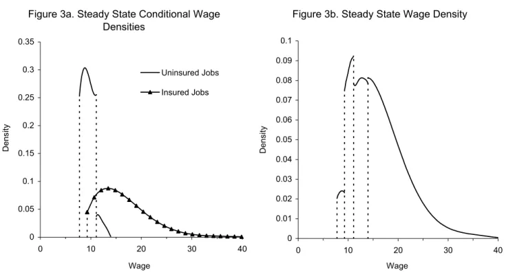
Figure 3 contains graphs of the simulated steady state conditional (on health insurance status) and unconditional wage distributions. The simulation on which these histograms are based is for one million labor market careers. The figures plot the equilibrium wage distributions from the model, i.e., they do not include measurement error.
Figure 3.a plots the steady state conditional wage distributions. For individuals in jobs covered by health insurance the shape of the distribution is rather unremarkable. The lowest value of the wage in this case is $9.12 using point estimates of the model parameters. The steady state wage distribution for individuals holding jobs not providing health insurance is more unusual. We know that this distribution is bounded, and we note a precipitous drop in the “density” at relatively high wages in the support of the distribution. This drop is due to the small proportion of histories that could lead to such a high wage rate. For an individual to have a high wage without health insurance implies that he is working at a firm with a relatively high value of θ but one that is less thanθ∗∗. If he is getting a high share of the surplus at this match, thisfirm has to bid against other firm(s) with match values less thanθbut sufficiently close to it. In our case, since the critical match value is 13.95, the highest wage that could possibly be observed without health insurance is $13.95.
The unconditional steady state wage distribution is plotted in Figure 3.b. As is to be expected, the upper tail of the density has a shape solely inherited from the relevant part of the conditional (on health insurance) wage density. Overall, the density is not very much at odds with what we typically observe in cross-sectional representative samples. The one possible exception to this claim pertains to the small but perceptible notches above and below the interval of overlap in the support of the two conditional wage distributions. These discontinuities in the density would be hidden if any amount of measurement error was added to the model, as it is when constructing the econometric specification below.
insurance, there are two possible routes by which any job spell can end. Given the efficient separa-tions implied by the search and bargaining process in the absence of firm heterogeneity, we know that voluntary exits from a job spell occur whenever a job with a higher match value is located (independent of whether the current job provides health insurance or not). For the model with no worker orfirm heterogeneity, the instantaneous exit rate from a job with match valueθ(θ≥θ∗) is given by
r(θ) =η0χ[θ∗≤θ < θ∗∗] +η1χ[θ≥θ∗∗] +λeG˜(θ), (12) so that the duration of time that individuals spend in a job spell conditional on the current match value is
fe(te|θ) =r(θ) exp(−r(θ)te), te>0.
Then the density of durations in a given job spell conditional upon health insurance status is
fe(te|d) =
Z
fe(te|θ)dG(θ|d).
The corresponding conditional hazard, he(te|d) =fe(te|d)/F˜e(te|d),exhibits negative duration
de-pendence for bothd= 0andd= 1.However, becauseη0> η1 and because the lowest value ofθfor
d= 1exceeds the greatest value ofθ ford= 0,the hazard out of jobs covered by health insurance exceeds the hazard out of jobs with health insurance for any value ofte.Note that the limiting value
(aste→ ∞)for the hazard in jobs without health insurance islimt→∞he(te|d= 0) =η0+λeG(θ˜ ∗∗),
while the corresponding limiting value for jobs with health insurance islimt→∞he(te|d= 1) =η1.
The job exit rates conditional on the current wage as well as health insurance status also have interesting properties. For simplicity, consider the exit rate from the first job following an unemployment spell (outside options are identical for these types of spells in a model with no individual orfirm heterogeneity). For a given(w, d)the hazard out of the job will be constant. We can write the hazard as
r(w, d) =ηd+λeG(θ(w, d)).˜ 8 (13)
If it was the case that there was no overlap in the supports of the conditional wage distributions by health insurance, then w would be a sufficient statistic for the rate of leaving the job since we could write d(w) ⇒ r(w, d) = r(w, d(w)) = r(w). However, with overlap in the support of the conditional wage distributions this is no longer the case and the pair (w, d) are required to completely characterize the job exit rate. We illustrate this point in Figure 4. For the set of wages consistent with either health insurance state, the value of dprovides information on the value of
θ associated with the match. For example, individuals paid $10 an hour could be receiving health insurance or not. Those with health insurance are less likely to leave the job both because they are less likely to receive a negative health shock but also because the θ value associated with a wage of 10 and health insurance is greater than theθ value associated with a wage of 10 and no health insurance. In contrast with claims in the empirical literature on job lock, the fact that the hazard rate out of a job that is covered by health insurance is lower than the exit rate from one that is not (conditional on the wage or not) does not necessarily indicate that health insurance status distorts the mobility decision.
8We are assuming that(w, d)are the wage and health insurance pair negotiated when entering the job from the
unemployment state. The individual can meet other potential employers that will not lead to a move but will result in a renegotiation in the wage. Allowing for renegotiations leads to a more complex mapping between the current (w, d)pair andθ. In this case, the mapping will be random rather than determinstic.
3
Data and Descriptive Statistics
Data from the 1996 panel of the Survey of Income and Program Participation (SIPP) are used to estimate the model. The SIPP interviews individuals every four months for up to twelve times, so that at most an individual will have been interviewed (relatively frequently) over a four year period. The SIPP collects detailed monthly information regarding individuals’ demographic characteristics and labor force activity, including earnings, number of weeks worked, average hours worked, as well as whether the individual changed jobs during each month included in the survey period. In addition, at each interview date the SIPP gathers data for a variety of health insurance variables, including whether an individual’s private health insurance is employer-provided.9 With the exception of the private demand for health insurance, the primitive parameters of the model developed in this paper are assumed to be independent of observable individual characteristics. Though in principle it would not be difficult to allow the primitive parameters to depend on observables, we instead have attempted to define a sample that is relatively homogeneous with respect to a number of demographic characteristics. In particular, only white males between the ages of 25 and 54 with at least a high school education have been included in our subsample. In addition, any individual who reports attendance in school, self-employment, military service, or participation in any government welfare program (i.e., AFDC, WIC, or Food Stamps) over the sample period is excluded.10 Although the format of the SIPP data makes the task of defining job changes fairly difficult, in other respects the survey information is well-suited to the requirements of this analysis since it follows individuals for up to four years and includes data on both wages and health insurance at each job held during the observation period.
Table 1 contains some descriptive statistics from the sample of individuals used in our empirical analysis. In Table 1.a we see that the sample consists of 10,121 individuals who meet the inclusion criteria discussed above. So as to minimize difficult initial conditions problems, the unit of analysis is a labor market “cycle,” which begins with an unemployment spell, which could be right-censored (i.e., may not end before the observation period is completed), and ends with the following right-censored or complete employment spell, if there is one.11. We partition the full sample into two
subsamples, one consisting of individuals who experienced unemployment at some point during the observation period and the other consisting of those who did not.12 Approximately twenty-eight percent of the full sample, or 2,814 individuals, fall into the former group. For these individuals, we use information regarding the duration of time spent in the initial unemployment spell, the duration of time spent in thefirst job spell after the unemployment spell, and the wage and health insurance status of thefirst two jobs in the employment spell following unemployment. In addition, 9There are several issues involved in constructing a meaningful employer-provided health insurance variable. First,
there is a timing problem since the insurance variable can change values only at the interview months, while a job change can occur at any time over a four month period. Second, there are job spells in which the individual reports employer-provided coverage for some part of the spell and no coverage for the remainder of the spell. We have made a good faith effort to accurately match job and health insurance spells, but we have been forced to make several judgment calls while constructing the event history data set.
1 0
Some individuals, about 3 percent of the sample, had missing data at some point during the panel. Since estimation depends critically on having complete labor market histories we have excluded these cases as well.
1 1
This approach was also taken by Wolpin (1992) and Flinn (2002).
1 2
The sample window is the length of time an individual remains in the SIPP. While the maximum length of the sample window is four years (or 208 weeks), a majority (52%) of sample members do not participate in all 12 waves of the survey. We measure the sample window from the initiation of the survey until the individual first fails to complete the survey.
we use marital status and children dummies as observable factors that influence the probability of having a high “private” demand for health insurance, and we use the length of the sample window as an exogenous factor that affects the probability of being observed in the non-employment state sometime during the panel. For the 7,307 individuals in the full sample whom we never observe in the unemployment state, we do not consider any labor market information but do include marital status and children dummies and the length of their sample windows when conducting the empirical analysis. It is interesting to note the differences among individuals in the two groups. Sample members without an unemployment spell over their sample window are much more likely to be married and to have children. The lengths of the sample windows are not very different for the two subsamples.
The labor market data from the sample members with an unemployment spell provide a wealth of information regarding the relationship between health insurance coverage, wages, and job mo-bility. From Table 1.b we observe that a slight majority (50.7%) of unemployment spells end with a transition into a job that provides health insurance. Perhaps the most striking feature of the data is the difference in the average wages of jobs conditional on health insurance provision. Jobs with health insurance have a mean wage 41 percent higher than jobs without health insurance. In addition, we see that individuals who exit unemployment for a job with insurance are more likely to be married with children than individuals who take a job without health insurance.
From the information on the first job following an unemployment spell, displayed in Figure 1.c, it is quite clear that jobs with health insurance tend to last longer on average than jobs without health insurance. Another feature of the data that is interesting to note is the difference in initial wages for the various transitions out of jobs with health insurance. In particular, while the mean initial wage for all insured jobs is almost $16, individuals who subsequently move into a job without insurance are earning $11.41 on average. In addition, the mean wage in the subsequent uninsured job is $16.14, well above the mean wage for uninsured jobs accepted directly out of unemployment. Finally, note the difference in the average wages of insured and uninsured jobs that follow a job without insurance (Figure 1.d). Jobs without insurance have a mean wage that is almost 6 percent larger than jobs with insurance. This is in marked contrast to the relationship between the average wages by health insurance status that are observed directly following an unemployment spell. The model constructed above is, on the face of it, consistent with all of these descriptive statistics, and in the following section we describe our attempt to recover the primitive parameters of the model from these data.
4
Econometric Speci
fi
cation
As noted above, the information used in the estimation process is best defined in terms of what we will refer to as an employment cycle. Such a cycle begins with an unemployment spell and is followed by an employment spell, which itself consists of one or more job spells (defined as continuous employment with a specific employer). Under our model specification we know that wages will generally change at each change in employer and can also change during a job spell at the time an alternative offer arrives that does not result in mobility but that does result in renegotiation of the employment contract. In terms of our model, an employment cycle is defined in terms of the following random variables
where tu is the length of the unemployment spell, tek is the length of the job spell with the kth
employer during the employment spell,wm is themth wage observation of theM that are observed
during the employment spell,tw
m is the time that themthwage came into effect,dq is theqthhealth
insurance status observed during the employment “cycle” of theQ distinct changes in status, and
tdq is the time that the qth health insurance status came into effect. Note that the total length of the employment spell (i.e., which is the length of the consecutive job spells) iste=Pktek and the
number of observed wages during the employment spell is at least as great as the number of jobs, orM ≥S. The {dq}q=1Q is an alternating sequence of 10s and 00s. Since we are assuming that no unemployed searcher will purchase health insurance, the process always begins with a 0 (since an employment cycle begins in the unemployment state). Other restrictions on the wage and health insurance processes will apply depending on the specification of searchers’ utility functions and the form of population heterogeneity.
Because of the unreliability of wage change information over the course of a job spell, in our estimation procedure we only employ wages observed at the beginning of a job spell and in terms of duration information we only use information on the duration of unemployment spells and the duration of job spells. Furthermore, to reduce the computational burden we consider (at most) the
first two jobs in a given employment spell.
As is often the case when attempting to estimate dynamic models, we face difficult initial conditions problems. In our framework, and common to most stationary search models, entry into the unemployment state essentially “resets” the process. While we will utilize all cases in the data in estimating the model, our focus will be on those cases that contain an unemployment spell. The likelihood function is written in terms of the employment cycles referred to above, so that only those cases that contain an unemployment spell are “directly” utilized. LetΨtake the value ‘1’ if a sample member experiences an unemployment spell at some point during their observation period and let it take the value ‘0’ when this is not the case. At the conclusion of our discussion of the likelihood contributions for sample members withΨ= 1we will derive the likelihood of this event. For present purposes we simply state that it is a function of the length of the sample period, which we will denote T, and the individual’s type ξ. Then let us denote P(Ψ= 1|ξ, T) by ωξ(T). It is assumed that the length of the sample window is independently distributed with respect to all of the outcomes determined within the model.
For the sample cases in which Ψ= 1the data utilized in our estimation procedure is given by
{tu, tj1, w1, w2, d1, d2}, where the two wage and health insurance status observations are those in effect at the beginning of the relevant job spell. The likelihood for these observations is constructed using simulations of the equilibrium wage and health insurance process in conjunction with clas-sical measurement error assumptions regarding observed beginning of spell wage rates and health insurance statuses. In particular, corresponding to any “true” wage w that is in existence at any point in time we assume that there is an observed wage given by
˜
w=wexp(ε), (14)
whereεis an independently and identically (continuously) distributed random variable. Our econo-metric specification will posit that εis normally distributed with mean 0, so that
ln ˜w= lnw+ε, (15)
and E(ln ˜w) = lnw. In terms of the observation of health insurance status, we will assume that the reported health insurance status at any point in time,d˜, is reported correctly with probability
γ and incorrectly with probability1−γ, independently of the actual state. Thusγ=p( ˜d= 1|d= 1) =p( ˜d= 0|d= 0).
Measurement error essentially serves three purposes in our estimation framework. First, it reflects the reality that there is a considerable amount of mismeasurement and misreporting in all survey data (though admittedly it is not likely to be exactly of the form we assume). Second, it serves to smooth over incoherencies between the model and the qualitative features of the data. For example, under certain specifications of the instantaneous utility function the model implies that the probability of moving directly from a job covered by health insurance to a job without insurance is a probability zero event. Data exhibiting such patterns will produce a likelihood value of 0 at all points in the parameter space. Measurement error makes such observations possible at all points in the parameter space.
The third usage is related to the simulation method of estimation. This method is most effective when based on a latent variable structure. In our case, the latent variables correspond to the simulated values of the variables that appear in the likelihood function, which themselves have a simple mapping into the observed values as a result of our i.i.d. measurement error assumptions. Thus any simulated value will have positive likelihood no matter what the observed value. In this sense, measurement error serves as a “smoother” of the likelihood. Because of its particular properties, measurement error is not introduced into the duration measures. By the structure of the model, it is not necessary to smooth the likelihood with respect to this information.
Throughout the empirical section we assume that the distributions of individual demands and
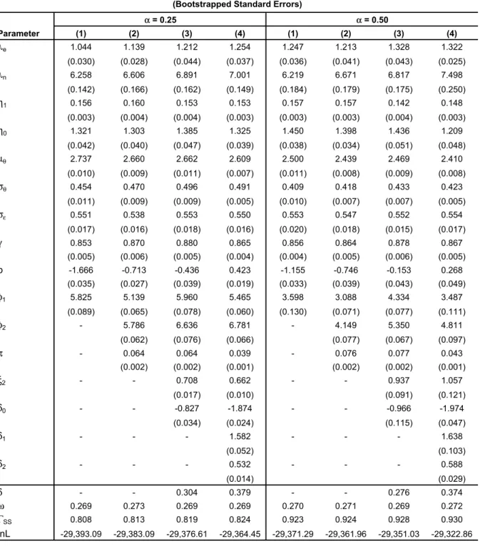
firm costs are both discrete. Firm cost types assume the values 0< φ1 < φ2,with the probability that a randomly selectedfirm has a high cost of providing health insurance given byPF(φ=φ2) =π.
On the individuals’ side of the market, we assume that there are two levels of private demand, with
0 = ξ1 < ξ2, and with the probability that the individual has a positive “private” demand for health insurance given byPH(ξ =ξ2) =δ.
The unit of analysis in our likelihood function is the individual. Individuals may be heteroge-neous with respect to their private demand for insurance, though we do assume that their type does not change over the course of the sample period. This implies that the decision rules used by any given agent will be time invariant. Recall that for an individual of typeξ we denote the value of employment at a firm with match value θ and cost type φwhen the next best alternative is at match value ofθ0 at a firm of cost type φ0 by
ˆ
VξE(θ, φ, θ0, φ0).
The characteristics (θ, φ) correspond to those of the higher value employment contract (from the point of view of the individual). In the presence offirm heterogeneity it need not be the case that
θ≥θ0,as is true when φ=φ0.
Corresponding to each set of state variables (θ, φ, θ0, φ0)for an individual of type ξ is a unique wage and health insurance pair ( ˆwξ,dˆξ)(θ, φ, θ0, φ0). For an individual of type ξ at a current job
with characteristics(θ, φ)let the set of alternative matches that would dominate the current match be denoted by Ωξ(θ, φ). As we have demonstrated above, this set is always connected and can be parsimoniously characterized as follows. For any type ξ agent with a current match (θ, φ), a potential match (a, b) dominates when
a >¯θξ(θ, φ, b).
employer, then
θ= ¯θξ(θ, φ, φ)
for any type ξ. On the other hand, whenφ6=bwe have
¯
θξ(θ, φ2, φ1) ≤ θ ¯
θξ(θ, φ1, φ2) ≥ θ.
The individual’s type will affect the size of the match differential required for a move to take place in these cases, though even individuals with no private demand for health insurance(ξ= 0)generally demand some differential.
Among the sample members for whom Ψ= 1we will discuss three qualitatively distinct cases. The first case, in which the observation period ends while the individual is still in an on-going unemployment spell, is the simplest. In this situation, the only contribution to the likelihood is the density of the right-censored unemployment spell. We will then discuss the second case, in which the individual has one job spell in the employment cycle, either due to the fact that he moves into unemployment at the conclusion of the first job spell or due to the fact that the first job spell is right-censored. In this case the likelihood contribution is defined with respect to the density of the completed unemployment spell, the observed wage and health insurance status at the initiation of thefirst job, and the length of the first job (be it censored or not). Thefinal case is that in which the individual has two consecutive job spells following the completion of an unemployment spell. In this case, the likelihood contribution is defined with respect to the duration of the unemployment spell, the duration of the first job spell, and the wages and health insurance statuses associated with the first two jobs (at their onset). We shall now consider these cases in the order of their complexity.
4.1
Unemployment Only
Recall that as long as an individual of type ξ would accept some match values at each type offirm (differentiated in terms ofφ) that would not result in the purchase of health insurance, the critical job acceptance match value for a type ξ person is independent of φ. This value is denoted by θ∗ξ. Then the hazard rate associated with unemployment for an individual of type ξ is given by
huξ =λnG(θ˜ ∗ξ), (16)
and the density of unemployment spell durations for a type ξ individual is
fξu(tu) =huξexp(−huξtu), (17)
where tu is the duration of the unemployment spell in the observation period. Since the hazard
function out of unemployment is constant given the individual’s type, it is irrelevant whether or not we observe the beginning of the unemployment spell.13 Then the probability that an unemployment spell of duration tu is on-going at the end of the sample period (e.g., is right-censored) given the
individual’s type is
1 3In a stationary model such as this one, the distribution of forward recurrence times of length-biased spells (i.e.,
those in progress at the time the sample window begins) is the same as the population distribution of completed spells (that are not length-biased). In our case, both distributions are negative exponential with parameterhu
L(1)ξ (tu,Ψ= 1|T) =ωξ(T) exp(−huξtu). (18)
Let the probability that the individual is a “high demand type” be denotedδ. Then the empirical likelihood in this case is given by
L(1)(tu,Ψ= 1|T) =δL(1)ξ 2 (t u,Ψ= 1 |T) + (1−δ)L(1)ξ 1 (t u,Ψ= 1 |T). (19)
4.2
One Job Spell Only
For all likelihood contributions that involve job spells we utilize simulation methods. We will describe the process by which we generate one sample path for an employment spell; for each individual in the sample we constructRsuch paths. If the minimum acceptable wage with each type of employer is the same, then the distribution of match draws in the first job spell is independent of the type of firm at which the individual finds employment. We simulate the match draw at the first firm by first drawing a value ζ1 from a uniform distribution defined on [0,1], which we denote byU(0,1). The match draw itself comes from a truncated lognormal distribution with lower truncation point given by the common reservation wage θ∗ξ. We have
θξ(ζ1) = exp(µ+σΦ−1(1−Φ(
ln(θ∗ξ)−µ
σ )(1−ζ1))). (20)
The rate of leaving the unemployment spell is hu
ξ =λG(θ˜ ∗ξ), so the likelihood of the completed
unemployment duration oftu is
huξexp(−huξtu).14 (21)
Given that thefirm is a high cost firm, the wage and health insurance decision are given by
(wξ2, d2ξ) = ( ˆwξ,dˆξ)(θξ(ζ1), φ2, VξN), (22)
where the equilibrium valuesxjξ denote the value of choice x at the beginning of job spell 1 given a firm typeφj and an individual typeξ, and xξˆ denotes the equilibrium mapping from these state variables into the contract, where x = w, d. The critical value for leaving the first firm will be equal to θξ(ζ1) whenever another high cost employer is encountered, and otherwise is equal to ¯
θξ(θξ(ζ1), φ2, φ1) when a low costfirm is met. The likelihood that the first job ends due to a quit
of any kind is then
hqξ(ζ1, φ2) =λe(πG(θξ(ζ˜ 1)) + (1−π) ˜G(¯θξ(θξ(ζ1), φ2, φ1))). (23) Since the “total hazard” associated with thefirst job in the employment spell is simply the sum of the hazard associated with a voluntary quit and a involuntary one, we have
heξ(ζ1, φ2) =hqξ(ζ1, φ2) +ηd2
ξ (24)
When the first employer is a low cost firm the situation is symmetric. The equilibrium wage and health insurance decisions are given by
(wξ1, d1ξ) = ( ˆwξ,dˆξ)(θξ(ζ1), φ1, VξN). (25)
1 4Note that this density is the same whether the individual began the sample window in this spell or whether it
The critical value that will induce job acceptance at a competing low cost firm is θξ(ζ1), while a
higher match is in general required if the individual is to accept employment at a high cost firm. The rate of leaving this job for another employer is
hqξ(ζ1, φ1) =λe(πG(¯˜ θξ(θξ(ζ1), φ1, φ2)) + (1−π) ˜G(θξ(ζ1))), (26)
and the total rate of leaving this job is
heξ(ζ1, φ1) =hqξ(ζ1, φ1) +ηd1
ξ. (27)
If the first job in the employment spell is still in progress at the end of the sample period then it is right-censored and we have all of the information required to compute the likelihood contribution. Conditioning on the individual’s type for the moment, the likelihood value associated with this particular simulation is given by
L(2)ξ (tu,w1˜ ,d1, t1, c1˜ = 1,Ψ= 1|ζ1, T) =ωξ(T)×huξexp(−huξtu)
× {πf( ˜w1|wξ2)×p( ˜d1|d2ξ)×exp(−heξ(θξ(ζ1), φ2)t1)
+ (1−π)f( ˜w1|wξ1)×p( ˜d1|d1ξ)×exp(−heξ(θξ(ζ1), φ1)t1)},
where c1 = 1 if the first job spell is right-censored and is equal to 0 if not. The density f( ˜w1|w1)
is generated from the measurement error assumption, as is p( ˜d1|d1). The term exp(−heξ(ζ1, φ)t1)
is the probability that the first job spell has not ended after a duration oft1 given that it is with
a firm of typeφ.
To form the likelihood contribution for the individual we have to average over a large number of simulation draws and over the possible individual types. Since both averaging operations are linear operations it makes no difference in which order we perform them. Then define the likelihood contribution for an individual with observed characteristics(tu,w˜1,d˜1, t1, c1 = 1,Ψ= 1, T) by
L(2)(tu,w˜1,d˜1, t1, c1 = 1,Ψ= 1|T) =R−1 R X r=1 {δL(2)ξ 2 (t u,w˜ 1,d˜1, t1, c1= 1,Ψ= 1|ζ1(r), T) (28) +(1−δ)L(2)ξ 1 (t u,w˜ 1,d˜1, t1, c1 = 1,Ψ= 1|ζ1(r), T)},
whereζ1(r) is therth draw from the U(0,1)distribution.
For the case in which the first job spell is complete and ends in an unemployment spell, the conditional likelihood function is slightly different. The likelihood that an individual of typeξwith a first job draw of θ who is employed at a firm of type φ exits into unemployment at time t1 is
the density of durations into unemployment conditional on exiting into unemployment multiplied by the probability that the individual has not found a better job by time t1. This is simply the
survivor function associated with the “voluntary exits” density evaluated att1, so that the product
of these two terms is
ηdj ξ exp(−ηdj ξ t1)×exp(−hξq(ζ1, φj)t1) (29) = η(djξ) exp(−heξ(ζ1, φj)t1)