HACH: Heuristic Algorithm for Clustering Hierarchy
Protocol in Wireless Sensor Network
IMuyiwa Olakanmi Oladimejia,∗, Mikdam Turkeya, Sandra Dudleya
aSchool of Engineering, London South Bank University,
103 Borough Road, London SE1 0AA
Abstract
Wireless sensor networks (WSNs) require energy management protocols to ef-ficiently use the energy supply constraints of battery-powered sensors to pro-long its network lifetime. This paper proposes a novel Heuristic Algorithm for Clustering Hierarchy (HACH), which sequentially performs selection of inactive nodes and cluster head nodes at every round. Inactive node selection employs a stochastic sleep scheduling mechanism to determine the selection of nodes that can be put into sleep mode without adversely affecting network coverage. Also, the clustering algorithm uses a novel heuristic crossover operator to combine two different solutions to achieve an improved solution that enhances the dis-tribution of cluster head nodes and coordinates energy consumption in WSNs. The proposed algorithm is evaluated via simulation experiments and compared with some existing algorithms. Our protocol shows improved performance in terms of extended lifetime and maintains favourable performances even under different energy heterogeneity settings.
Keywords: Wireless Sensor Networks, Sleep Scheduling, Clustering, Heuristic Crossover, Coverage, Energy Heterogeneity
IThis paper is an extended, improved version of the paper (A Heuristic Crossover
En-hanced Evolutionary Algorithm for Clustering Wireless Sensor Network) presented at Evo-ComNet2016 and published in: Applications of Evolutionary Computation, 19th European Conference, EvoApplications 2016, Porto, Portugal, March 30 - April 1, 2016, Proceedings, Part I, LNCS 9597, pp. (251-266), Springer, 2016.
∗Corresponding author
Email addresses: [email protected](Muyiwa Olakanmi Oladimeji), [email protected](Mikdam Turkey),[email protected](Sandra Dudley)
1. Introduction
Recent progress in wireless communications and micro-electronics have con-tributed to the development of sensor nodes that are agile, autonomous, self-aware and self-configurable. These sensor nodes are densely deployed through-out a spatial region in order to sense particular event or abnormal environmental
5
conditions such as moisture, motion, heat, smoke, pressure etc in the form of data [1]. These sensors, when in large numbers, can be networked and deployed in remote and hostile environments enabling sustained wireless sensor network (WSN) connectivity. Hitherto WSNs have been used in many military and civil applications, for example, in target field imaging, event detection, weather
10
monitoring, tactile and security observation scenarios [2]. Nevertheless, sensor node distribution and network longevity are constrained by energy supply and bandwidth requirements. These noted constraints mixed with the common de-ployment of large numbers of sensor nodes must be considered when a WSN network topology is to be deployed. The design of energy efficient scheme is a
15
major challenge especially in the domain of routing, which is one of the key func-tions of the WSNs [3]. Therefore, inventive techniques which reduce or eliminate energy inadequacies that would normally shorten the lifetime of the network are necessary. In this paper, the authors present a method which balances energy consumption among sensor nodes to prolong WSN lifetime. Energy
resourceful-20
ness is uniquely obtained using two described mechanisms; firstly, cluster head (CH) selection using a generic algorithm (GA) is employed that ensures appro-priately distributed nodes with higher energies will be selected as CHs. Secondly, a Boltzmann inspired selection mechanism was utilized to select nodes to send into sleep mode without causing an adverse effect on the coverage.
25
The commonest routing protocols deployed to challenge the challenges dis-cussed above are generally classified into two classes, namely flat and hierar-chical. Flat protocols comprise the well-known Direct Transmission (DT) and Minimum Transmission Energy (MTE), which do not provide balanced sensor energy distributions in a WSN. The disadvantage of the MTE is that a remote
sensor normally employs a relay sensor when transmitting data to/from the sink and this results in the relay sensor being the first node to die. In the DT pro-tocol, the sink communicates directly with sensors and this results in the death of the remote sensor first. Consequently when creating WSNs, energy-efficient clustering protocols act as a pivotal factor for sensor lifetime extension.
Gen-35
erally, clustering protocols can perform better than flat protocols in terms of balancing energy consumption and network lifetime prolongation by employing data aggregation mechanisms [4, 5]. In WSNs, there are three types of nodes considered: the cluster-head (CH), member node (MN) and sink node (SN). The member node manages sensing of the raw data and utilizes Time Domain
40
Multiple Access (TDMA) scheduling to send the raw data to the CH. The CH must aggregate data received from MNs and forward the aggregated data to the SN through single-hop or multi-hop. CH selection can be carried out by the sensors individually, by the SN or can be pre-implemented by the wireless network designer. Here, CH selection is performed by the SN due to the fact
45
that the SN has sufficient energy and can perform multifaceted calculations. The problem of CH selection can be considered as an optimization issue where the methods have employed GA to solve. Here the authors define an objective function that evaluates the discrete solution and propose an innovative heuristic crossover which is enhanced by the knowledge of our problem.
50
In this paper, we present a new Heuristic Algorithm for Clustering Hierarchy (HACH) protocol that simultaneously performs sleeping scheduling and clustering of sensor nodes upon each round. For sleep scheduling operation, the authors have developed the stochastic selection of inactive nodes (SSIN). A protocol that imitates the Boltzmann selection process in GA was used to decrease the
num-55
ber of active nodes in each round by putting some nodes to sleep or into inactive mode so that energy could be conserved and network lifetime increased with-out harming coverage. We further developed the Heuristic-Crossover Enhanced Evolutionary Algorithm for Cluster Head Selection (HEECHS) protocol for the clustering operation. HEECHS uses the known information around the problem
60
way to produce improved CH configuration. This method described has some parallels with optimization algorithms known as Memetic Algorithm (MAs). This algorithm is a type of stochastic global search heuristics in which Evo-lutionary Algorithm-based techniques are mixed with local search technique to
65
improve the quality of the solutions proposed by evolutions [6]. Sleep scheduling and clustering algorithms work together to optimize network lifetime by har-monizing energy consumption amongst sensor nodes during the communication times. Energy consumption optimization is performed by selecting spatially distributed nodes with higher energy as CHs and additionally placing certain
70
nodes into sleep mode without harming coverage. TheHACH protocol proposed performs very well compared to protocols that use GA because it integrates knowledge of the problem into GA crossover operator.
The rest of the paper is organised as follows. Section 2 presents related work on energy conservation techniques and clustering protocols in the area of
75
energy-efficient wireless sensor networks. Section 3 describes the network and radio model assumptions that underlie the protocol presented. In Section 4 the authors describe our proposed algorithm under three pivotal operational phases, those being the sleep scheduling mechanism, clustering algorithm and the energy consumption calculation. Section 5 presents our experimental set-up,
80
performance procedures, results and discussion. Finally, Section 6 provided our conclusion.
2. Related Work
In WSN environments, sensor node sleep scheduling can be used as an energy conservation method for network lifetime extension. In [7], a coverage
maximiza-85
tion with sleep scheduling protocol (CMSS) that ensures network areas are fully covered by selected active sensors was presented. Each sensor exchanges infor-mation with its neighbouring sensors and sets a waiting time. During sensor waiting times, a sensor can receive a sleep message from neighbouring nodes. When a sensor receives these messages, it updates its own neighbour and cell
value table. If the minimum value of the cell value table of a sensor equals to one, it silently becomes an active node. Otherwise, it will wait for the waiting time to expire before it turns into an inactive node. An energy preserving sleep scheduling (EPSS) strategy allows each sensor to make decisions regarding going into sleep mode based on their distance from the cluster head and network
den-95
sity. This guarantees balanced energy consumption in the cluster by taking into account the density of node deployment and the network load while determining the sleep probability [8]. In [9], a probabilistic and analytical method was em-ployed to approximate the overlapping sensing coverage between a node and its neighbours. It also estimates when a node can be put into sleep without
jeopar-100
dizing expected coverage. The method is employed by the proposed scheduling and routing scheme to diminish control message overhead while considering the next mode (full-active, semi-active, inactive/sleeping) of sensor nodes.
Apart from energy conservation techniques, energy-efficient clustering pro-tocols can also be employed to reduce and balance energy consumption across
105
sensor nodes in WSNs to prolong lifetime [10, 11, 12, 13]. At the time of CH and non-CH selection, the Low-Energy Adaptive Clustering Hierarchy (LEACH) as-sumes that the energy of each sensor node is the same. The selection process is carried out probabilistically and the CH’s main role is to aggregate the data received from its cluster members and transmit the aggregated data directly to
110
the sink. Difficulties with this protocol arise because the location of the selected CH may be some distance from the sink, thus it will consume more energy when transmitting to the sink. This can then result in CH nodes dying faster than other nodes [5]. A two-level LEACH (TL-LEACH) described in [14], adds an extra level to the cluster whereas LEACH has only one level. This additional
115
level diminishes energy consumption particularly for CHs quite a distance away from the sink. The hybrid energy efficient distributive (HEED) protocol pro-posed in [15] selects CHs by employing residual energy and the least amount of energy used for communication between the CHs and non-CHs. The sink accepts data from the nodes using a multi-hop communication approach.
120
[16], many nodes can consider themselves CH node candidates and inform other nodes of this. Every candidate CH node then examines if the other candidate CH nodes have a higher residual energy level or not. If there are none with higher residual energy, the highest announces itself the CH. The CH which has
125
the minimum-cost distance between itself and the CH to the sink is selected by non-CHs. The size of the cluster is balanced by the TCAC protocol and data is then sent directly to the sink from the CH. Within the proposed scalable energy efficient clustering hierarchy (SEECH) protocol [17], network nodes are sepa-rated into three layers, those being the member nodes, CH nodes and relays.
130
Clusters evolution is based on how central the CH node is with minimum intra-cluster energy distribution. A node close to the sink in a intra-cluster is often selected as the relay node. The CH node is assisted by the relay node to transmit ag-gregated data to the sink through hop or multi-hop communication. A genetic algorithm based energy efficient cluster (GABEEC) protocol was described in
135
[18]. Here clustering with dynamic CH selection was employed. An associate member node becomes a CH at the end of each round with this decision based on the remaining energy of the current CHs and the average energy of cluster members. The Genetic algorithm approach was described and was aimed to diminish communication distances and optimize network lifetime. Another
pa-140
per discussed a centralized energy-aware cluster-based protocol to extend the network lifetime of sensors by employing Particle Swarm Optimization (PSO) algorithm in [19]. The authors also defined a new cost function that simulta-neously accounts for the maximum distance between the non-CH node and its CH, and the remaining energy of CH candidates in the CH selection algorithm.
145
3. Network and Radio Model Assumptions
In theHACHprotocol proposed, important network and radio model assump-tions are presented as follows:
• The data sink is a stationary and resource-rich device that is placed far away from the sensing field.
• All sensors are stationary after deployment and average energy is constant in either homogeneous or heterogeneous environment.
• All sensors have GPS or other location determination devices attached to them. Hence, theHACHalgorithm can not be deployed for GPS-free sensor applications.
155
• Nodes are able to perform in inactive mode or a low power sleeping mode.
• Nodes that are close to each other have correlated data.
• The communication channel considered is assumed symmetric (i.e. the energy needed to transmit data from sensor node s1 to sensor node s2 is equal to the energy required to transmit a message from node s2 to node
160
s1 for a particular signal to noise ratio (SNR)).
To ensure just comparison with previous protocols [5, 20, 21], the authors have employed the simple model for the radio hardware energy dissipation where the transmitter dissipates energyET x(k, d) to manage the radio electronics and
the power amplifier, and the receiver dissipates energyERx(k) when managing
the radio electronics, as shown in Figure 1. The free space (d2 power loss) and
the multipath fading (d4 power loss) channel models were used (depending on
the distance (d) between the transmitter and receiver) for all the experiments described. The power-amplifier is fittingly managed so that should the distance be less than a threshold distance, we employ the free space (f s) model; else, the multipath (mp) model is used. Thus, to transmit a k-bit message a distanced,
Algorithm 1ProposedHACHProtocol
LetAliveN odes be the total number of sensor nodes
Computethe network total coverage.
while(AliveN odes >0)do
UsealgorithmSSINto select inactive nodes. (See Algorithm 2)
Putselected nodes into sleep mode.
Applythe proposedHEECHSalgorithm for CHs configuration. (See
Algo-rithm 3)
Computethe energy values of ECH,EM em andERes. (refer to Section
4.3.3)
Calculatethe number of dead nodes (node with energy equal or less than
0).
UpdateAliveNodes.
end while
the radio spends:
ET x(k, d) = kEelect+εmpkd4, ifd > d0 kEelect+εf skd2, ifd < d0 (1)
And to receivek-bit message, the radio uses:
ERx(k) =kEelect (2)
Where the equationd0= p
εf s/εmpsignifies the threshold distance and the
elec-tronics energy, factors such as the digital coding, modulation employed as well as filtering, and spreading of the signal effectEelect. The amplifier energy,εmp
orεf sdepends on the distance to the receiver and the acceptable bit-error rate.
165
4. The Proposed HACH Protocol
There are three consecutive operations within the proposed protocol: sleep scheduling, clustering and network operations. The sink transmits control pack-ets at the initial set-up phase so that it can receive node information in terms
of the nodes ID, location and energy. TheSSINprotocol proposed dynamically
170
selects the nodes to send to sleep by generating an initial candidate list. This list is populated with nodes having lower energies than the average energy of all the nodes. Employing a stochastic process, a small number of nodes are subsequently placed into sleep mode without harming coverage. CH selection employingHEECHSis then completed on the remaining active nodes.
175
The proposed HEECHS protocol operates at the network layer of WSNs layered model presented in [22], which is similar to the Open System Inter-connection (OSI) network model. After nodes deployment, the sink transmits and receives control packets containing the coordinates and energy value of all nodes. Using the obtained sensor coordinates, the sink computes the
Eu-180
clidean distances between two adjacent nodes and each node to the sink. These Euclidean distances and energy values are both used in establishing the cluster-based network topology for the purpose of packet routing.
Here, the authors have considered clustering as an optimization problem which would be best accomplished using GA. Tournament selection, mutation
185
operator and the heuristic crossover are the genetic operators used in this ap-proach. The most suitable CH configuration which guarantees balanced energy consumption across the network topology is selected at every network operation round. The residual energy of each node is calculated at the end of each round. This computed value is then employed to calculate the average energy for the
190
next round. This cycle subsequently repeats until all network nodes are dead, as shown in Algorithm 1.
4.1. Sleep Scheduling Mechanism
In this section, we discuss the estimation of coverage by setting up a matrix that computes the number of nodes covering the area within each grid point.
195
Furthermore, we present our SSIN protocol that uses the energy values and coverage effect in deciding which nodes to send into sleep mode.
4.1.1. Coverage Estimation and Matrix Setup
Coverage is estimated by dividing the sensing field into uniform grid areas. The number of sensors that cover each point on the grid is computed by
calcu-200
lating the euclidean distance between each grid point and the individual sensor’s point using their coordinates. If the euclidean distance between the two points is within the sensing rangeRs; the point is taken to be covered by the sensor.
The coverage matrix in Figure 2 helps to identify the grid points that are not covered by any sensor and the points covered by one or more sensors.
205 0 1 2 3 4 5 6 7 8 9 10 0 1 2 3 4 5 6 7 8 0 0 0 0 0 0 0 0 0 0 0 0 0 0 0 0 0 0 0 0 0 0 0 0 0 0 0 0 0 0 0 0 0 0 0 0 0 0 1 1 1 2 1 1 1 1 1 1 1 1 0 1 1 1 1 0 1 1 1 0 0 0 2 1 3 2 3 1 3 0 0 0 0 0 0 2 3 2 0 0 C A B D
Sensing Range Sensor Node
Figure 2: Coverage Matrix of covered grid points by sensors in 10×8 Sensing field
4.1.2. Inactive Node Selection usingSSIN mechanism
Conclusions as to which nodes to send into inactive mode at the beginning of each network operation round is made by theSSIN. The sleeping nodes can-didate list evolves through the inspection of which nodes have residual energy less than the computed average energy. This selection process is tantamount to the Boltzmann selection process whereby a method is adopted to control the selection pressure [23]. The temperature parameter is varied in the Boltzmann selection process to effectively control the selection pressure. The maximum cov-erage effect,M axef f is employed in this paper to regulate the effect of putting
WSN nodes to sleep and is defined as:
Here,Rsis the range over which a sensor node senses (taking the coverage area
as a circle with radiusRs), (pi×Rs2) is the coverage of one node and the value
020 represents coverage of two nodes.
The coverage effect Cef f as shown in Figure 3, is the effect of putting a
210
node to sleep based on coverage. The total coverage effect is computed by summoning a matrix called the Coverage Matrix. This matrix captures node coverage areas that overlap permitting the identification of nodes that can be placed into sleep mode without harming coverage as there will be other nodes covering the selected node’s area. The accumulated Coverage effect Accef f is
215
defined as the total effect on the coverage as a result of allowing some nodes to sleep. Our algorithm presented here has been created to ensure theAccef f value
is expected to be less than theM axef f for optimum coverage (Accef f<M axef f).
The probability that a node will be added to the sleeping node list can be computed using:
220
P =e(−Cef f/M axef f)/(1−(Accef f/M axef f)))2 (4)
Where the Accef f is the value to be minimized and M axef f is a control
parameter analogous to temperature in the Boltzmann tournament selection [24]. The computed probability,Pis compared to a randomly generated number in the range [0,1], uniformly at random. An inactive node candidate list is formed stochastically if therandom(0,1) is less thanP. Accef f is calculated by
225
adding its current value to theCef f value. TheSSINoperation continues until
Algorithm 2ProposedSSINprotocol
Accef f = 0;
Computethe residual energy,ERes of each node. (refer to section 4.3.3)
Computethe average energy of all nodes,EAvg.
Generatea candidate list for nodes that satisfies the conditionERes< EAvg.
ComputeM axef f. (refer to equation 3)
while(Accef f < M axef f)do
Computeprobability, P of adding nodes to the sleeping list. (See
equa-tion 4)
if (random(0,1)< P)then
Create list of sleeping node from the candidate list.
Computethe coverage effect,Cef f.
Accef f =Accef f +Cef f
end if end while
Accef f is larger than M axef f as described in Algorithm 2.
4.2. Clustering Operations usingHEECHS protocol
The clustering operation is divided into stages: CH selection, cluster for-mation, data aggregation and data communication. As shown in Figure 4, the
230
setup state starts by the CH selection stage and proceeds by cluster formation.
The setup state is followed by the data transmission state, which is subdivided into data aggregation and data transmission phases. During the setup state, a sink-assisted clustering algorithm that performs CH selection and membership association is applied to the active nodes in the network. An energy efficient
235
cluster-based topology is constructed by our proposed algorithm at every net-work operation round [2]. Sensors send their energy and location information to sink in order to implement the proposed algorithm. The HEECHS protocol favours selection of CH that has higher energy and far from neighbouring CH. Sensors are assigned to the closest CHs as member node, thereby forming cluster
240
as shown in Figure 5. TDMA schedule is assigned for each cluster to schedule packets transmission to CH by the member nodes. All the information about clusters and TDMA schedule packets is broadcasted to the network. Based on the time slot in the TDMA schedule packets, each node in a cluster send sensed data to respective CH.
245
Figure 5: WSNs Cluster-based Topology
At each round, the sink performs a re-clustering procedure to form a new cluster-based topology that preserves the WSNs coverage and energy efficiency characteristics by rotating the CH role among sensors with scalability of hun-dreds to thousands. Scalability implies that there is a need for balanced energy consumption among the sensor nodes during communication through an
cient clustering algorithm [25]. The CH loses energy faster than the member nodes; hence the need for re-clustering or rotating the CH role among sen-sors in order to balance the energy consumption. Re-clustering is performed at the end of a round, which is the total time span for a processes involved in the setup and steady data transmission state. The time-length of each round
255
must be carefully decided because a large time length drains CHs energy and a short time-length result into overhead caused by frequent re-clustering [26]. The round time-length of our proposed algorithm adjust itself dynamically based on the number of active nodes in the WSNs.
In this work, the HEECHS protocol proposed is developed for the CH
se-260
lection task using a heuristic-based GA. It runs through a number of tasks, similar to conventional GAs, such as population strings creation, string evalua-tion, best string selection and finally reproduction to create a new population. The unique, but significant difference is that the HEECHS protocol employs a problem-dependent knowledge-based heuristic crossover to find the best CH
265
configuration with the optimum number of appropriately distributed CH nodes.
In the proposedHEECHS, the genetic process of finding the best solution is per-formed using an energy unlimited sink device that can handle high execution time complexity and computation. The individuals within populationP(t) are coded by 0−1 binary representation where ’0’ denotes a member node and ’1’
270
denotes a CH node as shown in figure 6 below.
Each individual with lengthNsin a population sizepsis evaluated by
com-puting the fitness value using Equation 6. Individuals with the best fitness value are selected from two randomly selected parent pairs,P(x) andP(y). This pro-cess continues until the mating pool is filled. The heuristic crossover proposed
275
here is subsequently applied to the individuals in the pool and a new population
P(t+ 1) is produced. Again, each individual fitness value in this new population is computed using Equation 6 and the entire cycle continues until the stopping criterion is achieved. The stopping criterion is realized when the populations average fitness undergoes no further changes.
280
4.2.1. Proposed Objective Functions
To solve the CH selection problem, objective functions are developed because CH selection is considered an optimization problem. These objective functions return fitness values which are employed to assess the quality of a candidate solution. An objective function is found by taking into account parameters
285
such as the total sensor node energy and the Risk penaltyR. The sensor node energy parameter is considered to ensure that nodes with greater energy are given higher priority in the CH selection process.
The Risk penalty, R for the CH selection is defined as:
R= Lower−L, ifL < Lower L−U pper, ifL > U pper 0, otherwise (5)
Based on many iterative tests, the percentage of CHs number (L) to the total
290
between aLower limit of 4% andU pperlimit of 6%. Restrictions are imposed on the number of CHs using the parameterR.
Subsequently, the objective function is computed using:
F(X) =w1∗
AvgEN CH
AvgECH +w2∗R (6)
Wherew1andw2are the weighting factors. The average energy of non-CHs, AvgEN CH is the energy summation of all member nodes divided by the total
295
number of member nodes (n−L) as given below:
AvgEN CH =
P
iεN CHEi
n−L (7)
Also, the average energy of CHs, AvgECH is the energy summation of all CH nodes divided by the total number of CHs (L) as given below:
AvgECH=
P iεCHEi
L (8)
In equation 6, the ratio AvgEN CH
AvgECH is given a higher weighting factor
(w1=0.9) than the Risk penalty,R (w2=0.1) because of its importance. (Note:
300
CH andN CH represent the set of all CHs and non-CHs respectively). 4.2.2. Proposed Heuristic Crossover
The principal operator used in the HEECHS protocol to produce new solu-tions is the heuristic crossover. This is a problem-dependent crossover that utilizes knowledge of a problem to fuse two potential resolutions, producing a
305
new solution. According to Lixin Tang [27], a heuristic crossover is an operator that makes use of parents’ inherent information to produce an offspring. In the canonical approach, individuals in a population are selected and two parent individuals are combined using the crossover operator to produce a pair of off-spring that will replace its parents. Correspondingly, there is no assurance that
310
an offspring would be superior to its parents in the canonical approach [28]. Contrarily, the heuristic crossover operator generates only one offspring from two or more parents and it is certain that the offspring would be of higher qual-ity than the parents. As shown in Algorithm 3, the proposed heuristic crossover
Algorithm 3Proposed Heuristic Crossover
Selecttwo individuals from the parent population.
Computeand keep the CH position in each individual inCH1 andCH2.
Computethe threshold distance, T (refer to Section 4.2.2)
Computethe union setCHall=CH1∪CH2
Obtainthe first CH positionCHall(1) in theCHall set.
Generatea new setCHnew and transfer theCHall(1) to it.
Computethe distance,Dbetween CH positions in the setsCH1andCH2.
while(D < T)do
if (CHall node energy< CHnew node energy)then
Discard the CH node. (i.e. do not add toCHnewset)
end if
Replacethe CH in theCHnew set
end while
Addto the CH in the setCHall into theCHnew set.
generates a single solution with CHs that are spatially distributed in the sensor
315
field and selects nodes with higher energy to be the CH.
The CH genes position in each individual of selected parent pair is computed. An array that holds the genes position in both parent pairs is expressed by
CH1 and CH2. We decided to define the threshold distance between any two
adjacent CH position as
√
(xmax−xmin)2+(ymax−ymin)2
n×0.04 , where the (xmin, ymin)
320
and (xmax, ymax) coordinates represent the minimum and maximum xy points
in the sensing field, (n×0.04) indicates 4% of all sensor nodes. A set CHall is
generated from the union of CH1 and CH2 (refer to Algorithm 3). The first CH position in the union setCHall is moved into a new set CHnew by default. As
shown in Algorithm 3, the decision to move successive CH positions from the
325
4.2.3. Other Operators
The efficacy of a genetic algorithm relies upon maintaining a balance be-tween the concept of exploration and exploitation. Exploration is provided by crossover and mutation while selection enables exploitation [29, 30]. The rest of
330
the operators used in our proposedHEECHSprotocol are discussed below:
• TheTournament selection operatorselects individuals with the best fitness from groups of individuals randomly chosen from the current population. The selection pressure depends on the tournament size of the operator. In order to reduce the selection pressure, a tournament size of two was used
335
for our algorithm and this process continues until the mating pool is full.
• The Mutation operator changes an individual (parent) with a mutation probability (pm) to produces one individual (offspring) with new fitness value.
The parent and child individuals in the initial population pool produced in
340
the previous step are arranged in ascending order based on their fitness value. Subsequently, individuals with minimum fitness values are selected and they form the next generations population. Thestopping criterion is achieved when there is no further change in the fitness value of the population.
4.3. Network Operations and Energy Consumption Computation
345
In this algorithm, the network operations is divided into the set-up and steady phase. At each round the energy consumption value is computed by examining what happens to each node during both phases.
4.3.1. Set-up Phase
The sink transmits and receives control packets from all nodes during the set-up phase in order to initiate the inter- and intra-communication. This control packetskCP contain short messages that wake up and requests IDs, positions
and energy level from all sensor nodes. As in Equation 2, the energyERx(kCP) is
energyET x(kCP, d) transmitting control packets containing information about
their IDs, positions and energy levels to the sink. The sink processes control packets and certain decisions are made, such as which nodes to send into sleep mode, which nodes will become CH and the membership association of each CH. All nodes also use energy ERx(kCP) to receive their status information
(whether CH or members) from the sink. The energy spent by all CHs to send TDMA schedules to their members is given as:
ET x(chi)(kCP, di−toM em) = X i=1 chi∗ kCPEelect+εmpkCPd4i−toM em, ifd < d0 kCPEelect+εf skCPd2i−toM em, ifd > d0 (9) And the members spent energy to receive the TDMA schedules from the CH is
350
computed by Equation 2.
4.3.2. Steady Phase
In the steady state, active nodes transmit and sense data in the form of packets k to their CH based on the TDMA schedule received from the sink. Within a cluster, each CH is always prepared to accept this sensed data from its members. All sensed data received by the CH is aggregated and converted into a single data stream before being transmitting to the sink for processing. The CH sensor transceivers spent energyEDA to perform the aggregation task
is calculated using Equation 11. The overall energy dissipated by all members to transmit sense data to their CHs is calculated using:
ERx(mi)(k) = X
i=1
mikEelec (10)
Wheremi represents the member nodes in the seriesi= 1,2,3, ..., n−L. nand L denote the total number of all sensor nodes and cluster heads respectively. The energy spent by the CH to aggregate sensed data from its members and itself is calculated using:
EDA(mi+1)(k) =kEDA∗( X
i=1
Lastly, the CH dissipates energy to send their aggregated data to the sink and this can be calculated using:
ET x(chi)(kCP, di−toSink) = X i=1 chi∗ kCPEelect+εmpkCPd4i−toSink, ifd > d0 kCPEelect+εf skCPd2i−toSink, ifd < d0 (12)
4.3.3. Total Energy Consumption
The overall energy spent by all CHs can be calculated using:
ECHs= 2∗ERx(kCP) +ET x(kCP, di−toSink) +ET x(kCP, di−toM em)
+ERx(m1)(k) +EDA(mi+1)(k) (13)
Where 2∗ERx(kCP) results from the fact that a CH dissipates energy twice,
when it receives requests for ID, position and energy levels; and secondly when it receives membership status information for cluster set-up from the sink via a control packet. The energy lost by the member node is calculated as:
EM em=ET x(kCP, di−toSink) +ET x(kCP, di−toCH) + 3∗ERx(kCP) (14)
Where 3∗ERx(kCP) expresses that energy is lost by each member node when
receiving control packets. 2∗ERx(kCP) is the same as explained above and an
additional loss occurs when receiving TDMA schedules from its CH. The total energy dissipated by all nodes is computed as:
ET OT AL=ECHs+EM em (15)
Note: Current residual energyERes of each node is calculated by subtracting
the total energy consumption from the residual energy of previous round.
355
5. Simulation Results
The performance of clustering protocols can be evaluated using different types of metrics [27]. In this work, a MATLAB simulation model was devel-oped to test the performance of our proposed algorithm in terms of lifetime
evaluation of sensor nodes. Our proposedHACH protocol is considered scalable
360
in sense that it improves its energy efficiency as the network size increases. To demonstrate this fact we compare the performance of our proposed proto-col with SEECH, TCAC and SEECH protoproto-cols using experimentsExpR0M100,
ExpR0M400,ExpR0M1000which represent 100, 400 and 1000 homogeneous sensor
nodes respectively and zero heterogeneous nodes in terms of initial energy value
365
(refer to Table 1). Also, Table 3 presents experiment ExpR25M0, ExpR50M0,
ExpR75M0, ExpR100M0 which has 25, 50, 75, 100 heterogeneous sensor nodes
respectively and no homogeneous nodes. Lastly, the authors conducted more experiments that mixed heterogeneous nodes with homogeneous nodes, namely experimentsExpR25M75, ExpR50M50,ExpR75M25. The communication
parame-370
ters used for all the experiments presented in Table 1 and 3 is shown in Table 2.
In addition to the simulation parameters in Table 2, the GA parameters are set as population size,ps=100 and mutation rate,pm= 0.05. RandM signify
the number of heterogeneous and homogeneous sensor nodes respectively. In
375
Table 1 and 3, µ represents the sensor nodes mean energy, σR and σM
rep-Table 1: Parameter settings for Homogeneous WSNs Scenarios
Experiment Parameter Number of Sensors Sink Coordinates Dimension Initial Energy (J) ExpR0M100 100 (50,175) 100×100 µ=0.5 σM=0 ExpR0M400 400 (50,200) 100×100 µ=0.5 σM=0 ExpR0M1000 1000 (50,350) 200×200 µ=1.0 σM=0
Table 2: Communication Parameters with Specified Values
Parameter Value
Electronics Energy,Eelect 50nJ/bit
Multipath Loss,εmp 0.0013pJ/bit/m4
Free space Loss,εf s 10pJ/bit/m2
Aggregation Energy,EDA 5nJ/bit/signal
Threshold Distance,d0 87m
Control Packet size,kCP 50
Packets size,k 400
resent the standard deviation of heterogeneous and homogeneous sensor nodes respectively. For all experiments in Table 3, the mean initial energyE0 used is
0.5J.
5.1. Stability Period and Network Lifetime
380
The stability period length (SPL) is the time range from the start of network operation until when the first node dies (FND) whereas the instability period
Table 3: Parameter settings for Heterogeneous WSNs Scenarios
Experiments Parameter Number of Heterogeneous Nodes (R) Number of Homogeneous Nodes (M) Sink Coordinates Dimension Initial Energy (J) ExpR25M0 25 0 (50, 175) 100×100 µ=0.5 σR=0.05 ExpR50M0 50 ExpR75M0 75 ExpR100M0 100 ExpR25M75 25 75 (50, 175) 100×100 µ=0.5 σR=0.05 σM=0 ExpR50M50 50 50 ExpR75M25 75 25
Table 4: Performance comparison of LEACH, TCAC and SEECH withHACH Experiment Protocol Performance Measure (Round) FND LND IPL ExpR0M100 (100 Nodes) LEACH TCAC SEECH HACH 726 933 1028 1064 1209 1006 1099 1167 483 73 71 103 ExpR0M400 (400 Nodes) LEACH TCAC SEECH HACH 685 948 1016 1235 1274 1071 1140 1307 589 123 124 72 ExpR0M1000 (1000 Nodes) LEACH TCAC SEECH HACH 672 725 1587 1789 2014 1664 2202 2010 1342 939 615 221
(IPL) is the timespan from the FND until the last node dies (LND). The WSN lifetime is the time range from the start of network operation until the last node dies, which exclude energy unlimited sink devices (refer to Section 3).
385
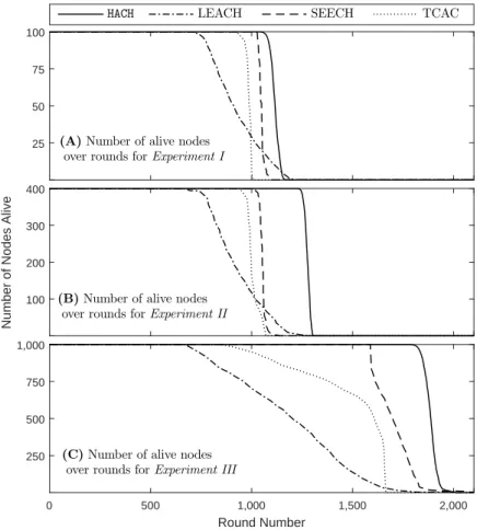
Immediately after the last sensor dies, the WSNs will stop its operation because the sink has lost its connectivity from the sensors. Alternatively, the WSNs lifetime can be defined as the combination of stability and the instability period. A reliable clustering process is characterized by a long SPL and a short IPL. Experimental results shown in Figure 7 depict the number of nodes that are
390
alive after each round.
The performance of our protocol is compared with other protocols in terms of the FND, LND, and IPL measures as seen on the graphs presented in Figure 7. Table 4 shows that ourHACHprotocol maintains the network operational lifetime of 338, 131 and 36 more than the LEACH, TCAC and SEECH respectively for
25 50 75 100
(A)Number of alive nodes over rounds forExperiment I
HACH LEACH SEECH TCAC
Number of Nodes Alive
100 200 300 400
(B)Number of alive nodes over rounds forExperiment II
Round Number 0 500 1,000 1,500 2,000 250 500 750 1,000
(C)Number of alive nodes over rounds forExperiment III
Figure 7: Lifetime evaluation ofHACH, LEACH, SEECH and TCAC
ExperimentExpR0M100. For a medium density WSN scenario ExpR0M400, our HACHshows a longer lifetime of 1235 rounds compared with LEACH, TCAC and SEECH which have a lower value of 685, 948 and 1016 respectively. The most fascinating result is that under the most dense WSNs (ExpR0M1000) containing
1000 sensors, our algorithm gives extremely high value of 1789 rounds compared
400
with 672, 725 and 1587 round of LEACH, TCAC and SEECH respectively. This shows that as the network size increases, the performance of HACH algorithm continues to improve.
it was deduced that HACH has a very low IPL values for larger network sizes
405
apart from ExperimentExpR0M100 which has 30 rounds more than the TCAC
protocol. This means thatHACH works very well in larger and denser network size. It is also noteworthy that the FND obtained in our proposedHACHprotocol forExpR25M0 (See Table 6) is 54 rounds more than LEACH protocol (refer to
ExpR100M0 in Table 1); which means that are protocol can still perform with
410
fewer nodes than the LEACH protocol.
5.2. Average Energy at First Node Dies (AEFND)
The AEFND is defined as the sum of all current or residual energy values of the sensor nodes divided by the number of nodes at the round when the first node dies. Many nodes begin to die when the first node dies and during the
415
instability periods because of the depleted energy supply. In theHACHprotocol, energies of some nodes are balance until the FND time and this is indicated on the graphs of Figure 7 by a sharp decline in the number of nodes that are alive forHACH, SEECH and TCAC protocol. One of the performance goals for an energy efficient protocol is to keep the AEFND to a very low value and our
420
HACHprotocol kept the AEFND to a very low value of approximately zero for all experiments as shown in Table 5 and 6. For example, ExperimentExpR0M100
has an AEFND of 0.0232J at FND time of 1064 as shown in Figure 8.
Table 5: AEFND of proposedHACHprotocol
Experiments
ExpR0M100 ExpR0M400 ExpR0M1000
AEFND 0.0232 0.0164 0.0650
This proves the fact that we were able to manage the energy usage until the FND time. The low AEFND values in Table 6 means that our protocol can
ef-425
0 500 1000 1500 2000 2500 0 0.1 0.2 0.3 0.4 0.5 x(rounds)
y(Average Energy of nodes alive)
Average Residual Energy FND
Figure 8: Average residual energy of nodes alive versus rounds (refer toExpR0M100)
Therefore, our proposed HACH reduces the energy consumed and enhances en-ergy balance across the nodes in the sensor field thereby extending the network lifespan.
5.3. WSNs Heterogeneity
430
After a certain number of rounds when the sensor networks lifetime has been depleted, new nodes are introduced to re-energize the sensor network. These new nodes are equipped with a higher constant energy value and nodes that are already in use have lower random energy, resulting in energy heterogeneity [31]. As shown in Figure 9, the FND value decreases from 1064 forExpR0M100(refer
435
to Table 4) to FND of 780 inExpR25M0(refer to Table 6). Despite the increase
in the ratio value of heterogeneous to homogeneous sensors from 25 to 100; which introduces more complexities in terms of energy imbalance, our protocol was still able to balance the energy consumption and maintain a constant FND value.
440
This phenomenon of starting a network operation with unbalanced energy distribution in a sensor networks is called WSNs heterogeneity. In this paper, the experiments that falls under the three level of energy heterogeneity are as follows:
• One-Quarter Level: ExperimentExpR25M0andExpR25M75.
445
Table 6: Performance Measures for different heterogeneous WSN Scenarios Experiment Performance Measures FND LND IPL AEFND ExpR25M0 780 937 157 0.040608 ExpR25M75 975 1126 151 0.033479 ExpR50M0 863 1010 147 0.033479 ExpR50M50 976 1061 147 0.030858 ExpR75M0 920 1059 139 0.033468 ExpR75M25 972 1123 151 0.030196 ExpR100M0 971 1110 139 0.033168
• Three-Quarter Level: ExperimentExpR75M0 andExpR75M25.
Each level has experiments with Full and Partial heterogeneity. Also, it can be observed in Table 6 that adding some energy-homogeneous sensor nodes to a set of energy-heterogeneous or energy depleted sensors extends the lifetime by
450
a considerable amount, for example experiments ExpR25M75, ExpR50M50 and
ExpR75M25 has a FND round of 195, 113 and 52 greater than experiments
0 25 50 75 100 0 200 400 600 800 1000 1200
Number of Heterogenoeus Sensors
R o u n d Nu m b er FND LND IPL
ExpR25M0, ExpR50M0 and ExpR75M0 respectively. The performance of each
experiment is compared withExpR100M0, and their percentage value is shown
on top of each bar as shown in figure 10.
455
5.3.1. Full heterogeneity
Full heterogeneity refers to a scenario whereby all the sensor nodes in a sensing field have random energy values and zero number of constant energy value. For example in Table 3, experiments ExpR25M0, ExpR50M0, ExpR75M0,
ExpR100M0are conducted using 25, 50, 75 and 100 number of sensor nodes with
460
random energy values and 0 constant energy values for all the experiments. The bar charts presented in figure 10 show that performance improves from one-quarter to the three-quarter full heterogeneity level when compared with ExpR100M0. In figure 10a, FND percentages of increasing order of 80.33%,
84.41% and 94.75% were obtained. Also, the LND percentage is in ascending
465
order of 84.41%, 90.99%, 95.41% as shown in figure 10b. Additionally the IPL percentage is in decreasing order of 112.95%, 105.76%, 100.0%; meaning the performance increased as the number of heterogeneous nodes increased. Also, in figure 10c,ExpR50M0 was able to obtain 105.76% which is the same value as
the half-levelExpR50M50.
470
5.3.2. Partial heterogeneity
This is the WSN scenario that describes the ratio combination of sensor nodes with random and constant energy values. In Table 6,ExpR25M75,ExpR50M50
andExpR75M25 use 25, 50, 75 sensor nodes with random energy and 75, 50, 25
sensor nodes with constant energy respectively. In figure 10a, the FND time for
475
ExpR25M75, ExpR50M50, and ExpR75M25 is 100.41%, 100.52% and 100.11%
re-spectively when compared withExpR100M0; showing that there is no significant
improvement as the ratio of heterogeneous to homogeneous nodes increases. In figure 10,ExpR50M50produces the most improved FND of 0.52% more than the
ExpR100M0and percentage reduction of LND by 4.41%.
One−Quarter Half Three−Quarter 0 200 400 600 800 1000 1200 Heterogeneity Level Round Number
Full Heterogeneity Partial Heterogeneity FND= 971 for Exp R100M0 80.33% 100.41% 88.88% 100.52% 94.75%100.11% (a) FND
One−Quarter Half Three−Quarter
0 200 400 600 800 1000 1200 1400 Heterogeneity Level Round Number
Full Heterogeneity Partial Heterogeneity LND= 1110 for Exp R100M0 84.41% 101.44% 90.99%95.59% 95.41% 101.17% (b) LND
One−Quarter Half Three−Quarter
0 50 100 150 200 Heterogeneity Level Round Number
IPL= 139 for Exp R100M0
105.76%105.76%
100.00% 108.63% 108.63%
112.95%
Full Heterogeneity Half Heterogeneity
(c) IPL
6. Conclusion
In this paper, we have proposed a new HACH algorithm. The algorithm re-duces and balances energy consumption by selecting distributed nodes with high energy as cluster heads to prolong network lifetime. Sequentially, this is achieved by two major operations such as sleep scheduling and cluster head selection
op-485
erations. TheSSINsleep scheduling mechanism inspired by Boltzmann selection process was proposed to decide which nodes to send into sleep mode with negligi-ble effect on the coverage. Subsequently, we employed a genetic algorithm-based technique called theHEECHSprotocol that would distribute cluster heads evenly within a sensor field to ensure that energy consumption is balanced across the
490
networks. To guarantee an efficient cluster head selection process, we designed an objective function to evaluate the quality of our solutions. Simulation results of the first three experiments shows that our proposedHACHalgorithm outper-forms the SEECH, TCAC and LEACH. Also, further experiments demonstrated that our protocols can perform even better under different heterogeneity levels
495
of wireless sensor network settings and still maintain acceptable performances.
References
[1] M. O. Oladimeji, M. Turkey, S. Dudley, A heuristic crossover enhanced evo-lutionary algorithm for clustering wireless sensor network, in: Applications of Evolutionary Computation - 19th European Conference,
EvoApplica-500
tions 2016, Porto, Portugal, March 30 - April 1, 2016, Proceedings, Part I, 2016, pp. 251–266.
[2] S. Naeimi, H. Ghafghazi, C.-O. Chow, H. Ishii, A survey on the taxonomy of cluster-based routing protocols for homogeneous wireless sensor networks, Sensors 12 (6) (2012) 7350–7409.
505
[3] A. Chakraborty, S. K. Mitra, M. K. Naskar, Energy efficient routing in wireless sensor networks: A genetic approach, CoRR abs/1105.2090.
[4] A. A. Abbasi, M. Younis, A survey on clustering algorithms for wireless sensor networks, Computer communications 30 (14) (2007) 2826–2841. [5] W. B. Heinzelman, A. P. Chandrakasan, H. Balakrishnan, An
application-510
specific protocol architecture for wireless microsensor networks, Wireless Communications, IEEE Transactions on 1 (4) (2002) 660–670.
[6] W. E. Hart, N. Krasnogor, J. E. Smith, Recent advances in memetic algo-rithms, Vol. 166, Springer Science & Business Media, 2005.
[7] C. Danratchadakorn, C. Pornavalai, Coverage maximization with sleep
515
scheduling for wireless sensor networks, in: Electrical Engineer-ing/Electronics, Computer, Telecommunications and Information Technol-ogy (ECTI-CON), 2015 12th International Conference on, IEEE, 2015, pp. 1–6.
[8] B. Singh, D. Lobiyal, Energy preserving sleep scheduling for cluster-based
520
wireless sensor networks, in: Contemporary Computing (IC3), 2013 Sixth International Conference on, IEEE, 2013.
[9] E. Bulut, I. Korpeoglu, Sleep scheduling with expected common coverage in wireless sensor networks, Wireless Networks 17 (1) (2011) 19–40. [10] S. H. Kang, T. Nguyen, Distance based thresholds for cluster head selection
525
in wireless sensor networks, Communications Letters, IEEE 16 (9) (2012) 1396–1399.
[11] L. YeMao, C. Fa, W. Hai, An energy efficient clustering scheme in wireless sensor networks, Ad Hoc & Sensor Wireless Networks (to be published). [12] N. Dimokas, D. Katsaros, Y. Manolopoulos, Energy-efficient distributed
530
clustering in wireless sensor networks, Journal of parallel and Distributed Computing 70 (4) (2010) 371–383.
[13] S. Lin, J. Zhang, G. Zhou, L. Gu, J. A. Stankovic, T. He, Atpc: adaptive transmission power control for wireless sensor networks, in: Proceedings of
the 4th international conference on Embedded networked sensor systems,
535
2006, pp. 223–236.
[14] V. Loscri, G. Morabito, S. Marano, A two-levels hierarchy for low-energy adaptive clustering hierarchy (tl-leach), in: IEEE Vehicular Technology Conference, Vol. 62, IEEE; 1999, 2005, p. 1809.
[15] O. Younis, S. Fahmy, Heed: a hybrid, energy-efficient, distributed
cluster-540
ing approach for ad hoc sensor networks, Mobile Computing, IEEE Trans-actions on 3 (4) (2004) 366–379.
[16] D. P. Dahnil, Y. P. Singh, C. K. Ho, Topology-controlled adaptive cluster-ing for uniformity and increased lifetime in wireless sensor networks, IET Wireless Sensor Systems 2 (4) (2012) 318–327.
545
[17] M. Tarhani, Y. S. Kavian, S. Siavoshi, Seech: Scalable energy efficient clustering hierarchy protocol in wireless sensor networks, Sensors Journal, IEEE 14 (11) (2014) 3944–3954.
[18] S. Bayrakli, S. Z. Erdogan, Genetic algorithm based energy efficient clusters (gabeec) in wireless sensor networks, Procedia Computer Science 10 (2012)
550
247–254.
[19] N. Latiff, C. C. Tsimenidis, B. S. Sharif, Energy-aware clustering for wire-less sensor networks using particle swarm optimization, in: Personal, In-door and Mobile Radio Communications, 2007. PIMRC 2007. IEEE 18th International Symposium on, IEEE, 2007, pp. 1–5.
555
[20] J.-L. Liu, C. V. Ravishankar, et al., Leach-ga: Genetic algorithm-based energy-efficient adaptive clustering protocol for wireless sensor networks, International Journal of Machine Learning and Computing 1 (1) (2011) 79–85.
[21] K. G. Vijayvargiya, V. Shrivastava, An amend implementation on leach
560
protocol based on energy hierarchy, International Journal of Current Engi-neering and Technology 2 (4) (2012) 427–431.
[22] W. Charfi, M. Masmoudi, F. Derbel, A layered model for wireless sensor networks, in: Systems, Signals and Devices, 2009. SSD’09. 6th International Multi-Conference on, IEEE, 2009, pp. 1–5.
565
[23] D. Dumitrescu, B. Lazzerini, L. Jain, A. Dumitrescu, Evolutionary Compu-tation, International Series on Computational Intelligence, Taylor & Fran-cis, 2000.
[24] D. E. Goldberg, A note on boltzmann tournament selection for genetic algorithms and population-oriented simulated annealing, Complex Systems
570
4 (4) (1990) 445–460.
[25] Q. Mamun, A qualitative comparison of different logical topologies for wire-less sensor networks, Sensors 12 (11) (2012) 14887–14913.
[26] V. Pal, G. Singh, R. Yadav, Analyzing the effect of variable round time for clustering approach in wireless sensor networks, Lecture Notes on Software
575
Engineering 1 (1) (2013) 31.
[27] T. Lixin, Improved genetic algorithms for tsp, JOURNAL OF NORTH-EASTERN UNIVERSITY (NATURAL SCIENCE) (1999) 01.
[28] B. S. Hasan, M. Khamees, A. S. H. Mahmoud, et al., A heuristic genetic al-gorithm for the single source shortest path problem, in: Computer Systems
580
and Applications, 2007. AICCSA’07. IEEE/ACS International Conference on, 2007, pp. 187–194.
[29] R. Halke, V. Kulkarni, En-leach routing protocol for wireless sensor net-work, International Journal of Engineering Research and Applications 2 (4) (2012) 2099–2102.
585
[30] J. Brunda, B. Manjunath, B. Savitha, P. Ullas, Energy aware threshold based efficient clustering (eatec) for wireless sensor networks, Energy 2 (4). [31] H. Kour, A. K. Sharma, Hybrid energy efficient distributed protocol for heterogeneous wireless sensor network, International Journal of Computer Applications 4 (6) (2010) 1–5.