research paper series

research paper series

Research Paper 2004/10

Intra-Industry Trade with Multinational Firms:

Theory, Measurement and Determinants

by

Hartmut Egger, Peter Egger and David Greenaway

The Centre acknowledges financial support from The Leverhulme Trust

The Authors

Hartmut Egger is Senior Assistant at the University of Zurich. Peter Egger is Professor of Economics at the University of Innsbruck. David Greenaway is Professor of Economics at the University of Nottingham and Director of the Leverhulme Centre for Research on Globalisation and Economic Policy (GEP).

Acknowledgements

David Greenaway acknowledges support from the Leverhulme Trust under programme grant F114/BF.

Intra-Industry Trade with Multinational Firms: Theory, Measurement and

Determinants

by

Hartmut Egger, Peter Egger and David Greenaway

Abstract

A number of recent developments, including the analysis of firm level adjustment to falling trade costs, have contributed to a revival of interest in intra-industry trade. Most empirical work still relies on the standard Grubel-Lloyd measure. This however refers only to international trade, disregarding income flows stimulated by repatriated profits. Given the overwhelming importance of the latter, this is a major shortcoming. We provide a guide to measurement and estimation of the determinants of bilateral intra-industry trade shares from the perspective of new trade theory with multinational firms. We develop an analytically solvable general equilibrium model to investigate investment costs, multinational activities and income flows from repatriated profits. The robustness of our findings are investigated in five simulation analyses. We also discuss and quantify biases of different Grubel-Lloyd indices in an empirical assessment of intra-industry trade shares and identify repatriated profit flows of multinationals as a key determinant of biased measurement. To overcome this, we provide several alternative, bias-corrected versions of the Grubel-Lloyd index. Finally, we demonstrate that the determinants motivated by our theoretical analysis offer important insights into variations in the Grubel-Lloyd index. Our new specification outperforms any other previously estimated model as illustrated in regressions on numerically generated data.

JEL classification: F12, F23

Keywords: intra-industry trade, multinationals

Outline 1. Introduction 2. Theoretical background 3. Empirical analysis 4. Conclusions

Non-Technical Summary

The publication of Grubel and Lloyd (1975) stimulated enormous interest in intra-industry trade (IIT), for two reasons. First, the empirical phenomenon of high levels of trade in products from similar industries between countries with similar factor endowments seemed to be at odds with the standard Heckscher-Ohlin-Samuelson (HOS) workhorse model of international trade. Second, the observed increase in intra-industry trade coincided with what appeared to be relatively painless adjustment to economic integration in western Europe. The dislocation anticipated as inter-industry specialisation occurred did not materialise, giving rise to the so-called ‘smooth adjustment hypothesis’.

In the decade that followed Grubel and Lloyd (1975) the literature exploded. Empirical analysis focused primarily on three things. First whether the phenomenon survived data disaggregation. Second, was IIT a peculiarity of trade in western Europe? Third, what were the drivers of the phenomenon?

Recent years have seen a revival of interest in intra-industry trade, stimulated by frontier work on trade costs, economic geography and a range of aspects of firm level adjustment to globalisation. One focus of this, from both a theoretical and measurement standpoint is intra-industry trade in a setting with multinational firms. This is a very important development from a theoretical standpoint because we have known for a long time that both phenomena co-exist, indeed are often co-terminous and we need good models for explaining this. But it is also important from a measurement perspective because of the importance of international production and intra-firm trade relative to armslength trade. FDI has grown about twice as fast as trade over the last decade. The principal sources and hosts are industrialised countries and two-way trade is closely associated with two-way FDI.

This paper contributes to this new literature in several ways. First, it generates a proof that the standard and still widely used Grubel-Lloyd index has to be adjusted to reflect more than the intra-industry trade share in a narrow sense. We build a general equilibrium model which shows that with multinational firms, both unbalanced profit repatriation and trade costs distort the index. We expose the biases resulting from these empirically relevant phenomena and construct several new versions of bias-corrected Grubel-Lloyd indices. Second, we develop a three-factor general equilibrium model of trade and multinationals to provide a detailed analysis of the role of investment cost differences between countries as a determinant of FDI and, hence, intra-industry trade. By introducing three factors, we emphasise the distinction between two important characteristics of headquarters: their provision of physical capital to set up plants, and the human-capital intensive generation of firm-specific assets through brand proliferation. Besides this more complete description of headquarter services, there is an advantage of analytical tractability since there are as many activities (homogeneous goods production, exporter and multinational production of manufactures) as there are factors (physical capital, skilled labour, unskilled labour). In this setting, we are able to evaluate not only the role of investment cost levels and differences in general but also their interaction with labour and capital endowments, depending on whether horizontal or vertical multinationals are active.

Third, a large number of numerical simulations of our model allow us to evaluate the robustness of our analytical findings with respect to simplifying assumptions as well as traditional determinants such as country size, capital-labour ratios and skilled-unskilled ratios.

Finally, we implement and report on an extensive empirical analysis, where uncorrected and bias-corrected versions of the Grubel-Lloyd index are used as regressors. This yields several conclusions. We find that biases not only affect the overall magnitude of the Grubel-Lloyd index but also systematically affect parameter estimates; cross-section estimates tend to be inconsistent if country-specific effects are excluded; the determinants generated by our theoretical model account for more than 50% of the variation in intra-industry trade-share data, implying that less than half of their variation is explained by traditionally used variables. Given the crucial importance of estimating accurately intra-relative to inter-industry trade, this is very significant.

1 Introduction

The publication of Grubel and Lloyd (1975) stimulated enormous interest in intra-industry trade (IIT), for two reasons. First, the empirical phenomenon of high levels of trade in products from similar industries between countries with relatively similar factor endowments seemed to be at odds with the standard Heckscher-Ohlin-Samuelson (HOS) workhorse model of international trade. Second, the observed increase in intra-industry trade coincided with what appeared to be relatively painless adjustment to economic integration in western Europe. The dislocation anticipated as inter-industry specialisation occurred did not materialise, giving rise to the so-called ‘smooth adjustment hypothesis’.

In the decade that followed Grubel and Lloyd (1975) the literature exploded. Empirical analysis focused primarily on three things. First whether the phenomenon survived data disaggregation. Finger (1975) famously described IIT as a ‘statistical artefact’, a mirage created by the vagaries of statistical classification. Greenaway and Milner (1983) among others showed that although shares of IIT in total trade declined as trade data became more finely disaggregated, it did not disappear. In fact it remained prevalent. Second, was IIT a peculiarity of trade in western Europe. Studies in Tharakan (1983) demonstrated that it was not. Although average levels were lower in developing, and what are now referred to as transition economies, they were non-trivial. Third, what were the drivers of the phenomenon? Early cross-section work such as Loertscher and Wolter (1980) and Greenaway and Milner (1984) pointed to various aspects of industrial organisation but findings were not robust. Indeed, an application by Torstensson (1996) of extreme bounds analysis confirmed that the cross-industry determinants were very fragile.

This, and other work, progressed thinking on measurement and to a lesser extent explanation. Innovations on the theoretical front were much more dramatic, with the development and refinement of models of monopolistic competition and international trade (most notably Lancaster 1980, Krugman 1979 and 1980 and Helpman and Krugman 1985) as well as strategic interaction and intra-industry trade (eg Brander 1981 and Brander and Krugman 1982). These offered convincing explanations of the market structures under which we would expect IIT to be generated and have proved to be of lasting value. Many, and in particular Krugman (1981), focused on distributional consequences, emphasising the likelihood of

greater symmetry between expanding and declining activities than in an HOS world and offering a theoretical underpinning to the potential for lower adjustment costs in an IIT setting as compared to HOS.

Recent years have seen a revival of interest in intra-industry trade, stimulated by frontier work on trade costs, economic geography and a range of aspects of firm level adjustment to globalization. One important focus of this, from both a theoretical and measurement standpoint is intra-industry trade in a setting with multinational firms. This is a very important development from a theoretical standpoint because we have known for a long time that both phenomena co-exist, indeed are often co-terminous and we need good models for explaining this. But it is also important from a measurement perspective because of the importance of international production and intra-firm trade relative to armslength trade. FDI has grown about twice as fast as trade over the last decade. The principal sources and hosts are industrialised countries and two-way trade is closely associated with two-way FDI.

An important development in understanding the relationship between IIT and intra-industry affiliate production is Markusen and Maskus (2001). From a specification based on numerical simulations of a two-factor knowledge capital model (associated with Carr et al., 2001 and Markusen, 2002), they find that intra-industry trade between the US and partner economies tends to decrease with greater similarity in size, which is at odds with the findings of Helpman (1987), Bergstrand (1990) or Hummels and Levinsohn (1995). They also found it decreased with the bilateral trade cost level, but increased with the bilateral level of investment costs. However, apart from these papers, this issue remains largely unexplored.

This paper contributes to this new literature in several ways. First, it generates a proof that the standard and still widely used Grubel-Lloyd index has to be adjusted to reflect more than the intra-industry trade share in a narrow sense. We build a general equilibrium model which shows that with multinational firms, both unbalanced profit repatriation and trade costs distort the index. We expose the biases resulting from these empirically relevant phenomena and construct several new versions of bias-corrected Grubel-Lloyd indices. Second, we develop a three-factor general equilibrium model of trade and multinationals to provide a detailed analysis of the role of investment cost differences between countries as a determinant of FDI and, hence, intra-industry trade. By introducing three factors, we emphasise the distinction between two important characteristics of headquarters: their provision of physical capital to

set up plants, and the human-capital intensive generation of firm-specific assets through brand proliferation. Besides this more complete description of headquarter services, there is an advantage of analytical tractability since there are as many activities (homogeneous goods production, exporter and multinational production of manufactures) as there are factors (physical capital, skilled labour, unskilled labour). In this setting, we are able to evaluate not only the role of investment cost levels and differences in general, but also their interaction with labour and capital endowments, depending on whether horizontal or vertical multinationals are active.

Third, a large number of numerical simulations of our model allow us to evaluate the robustness of our analytical findings with respect to simplifying assumptions as well as traditional determinants such as country size, capital-labour ratios and skilled-unskilled ratios.

Finally, we implement and report on an extensive empirical analysis, where uncorrected and bias-corrected versions of the Grubel-Lloyd index are used as regressors. This yields several conclusions. We find that biases not only affect the overall magnitude of the Grubel-Lloyd index but also systematically affect parameter estimates; cross-section estimates tend to be inconsistent if country-specific effects are excluded; the determinants generated by our theoretical model account for more than 50% of the variation in intra-industry trade-share data, implying that less than half of their variation is explained by traditionally used variables. Given the crucial importance of estimating accurately intra-relative to inter-industry trade, this is very significant.

The remainder of the paper is organized as follows: Section 2 sets out our theoretical model of intra-industry trade with investment costs and introduces a corrected Grubel-Lloyd index. This is subjected to simulation analysis and a number of theoretical propositions are derived. Section 3 sets up our econometric analysis, reports our results and subjects them to sensitivity analysis. Section 4 concludes.

2 Theoretical

background

2.1 The Grubel-Lloyd index

The Grubel and Lloyd (1971) index has become the standard measure for the intensity of intra-industry trade. In the two-country case, this is defined as1

(

)

2 min _ik, _ik k ik ik k k EX IM GLI EX IM × = +

∑ ∑

∑

, (1)

where EX_ik is the value of country i’s exports of good k. IM_ik represents expenditures for country i’s imports of good k. Although this has been the index of choice for most researchers in this area for over 30 years, it is an inappropriate measure if there are multinational

activities because does not account for (unbalanced) repatriated profits of multinational

firms and, therefore, underestimates the intra-industry trade share. For convenience, we use the term trade imbalance bias to refer to this measurement error.

GLI

(

)

EX

2 _{To see this bias, consider}

the case of two economies with one sector of production and multinational activities of country i firms in country j. From payments balance it follows that

, if there are flows of repatriated profits due to multinational activities of country i firms in j. Thus, GL

2 m× in EX_i,IM_i < _i +IM_i

1

I < , according to (1). However, in a one-sector model there is by definition only intra-industry trade, so that the correct GLI must equal one.

To obtain an appropriate measure of the IIT share, we have to adjust the Grubel-Lloyd index for all income flows not due to goods trade, like repatriated profits.3 _{More precisely, we}

correct the denominator of GLI for all output flows that are balanced by income flows not directly related to exports and imports. This gives a hypothetical measure of balanced trade in the denominator of GLI.4 The corrected Grubel-Lloyd index for the two-country, multi-sector case is then:

1 _{We do not distinguish between c.i.f and f.o.b data for the moment. For a rigorous discussion on different}

empirical specifications of the Grubel-Lloyd index see Subsection 3.1.

2 _{Note that this has an entirely different motivation than the case made by Aquino (1978) for a correction for}

aggregate payments imbalance. As Greenaway and Milner (1981) showed this is neither defensible on theoretical grounds nor practicable.

3 _{(See Subsection 3.1 and Appendix C for the quantification of this and other biases).}

4 _{This adjustment method was in fact first suggested by Grubel and Lloyd (1975). However, they did not develop}

(

)

2 min _ik, _ik C k ik ik ik ik k k k k EX IM GLI EX IM EX IM × = + − −

∑

_∑

_∑

_∑

_∑

, (2)

In our thought experiment with two one-sector economies and multinational activities of country i firms in country j, gives a correct measure of the intra-industry trade share,

i.e. .

C

GLI 1

C

GLI = 5 _{According to (1) and (2), we obtain}

: 1 C _{ik ik} k k ik ik ik ik k k k k EX IM GLI SHI GLI _{EX IM EX IM} − = = + + − − >1

∑

∑

∑

∑

∑

∑

(3)

as a measure of the trade imbalance bias in relative terms.

In what follows we are interested in the role of multinational activities and repatriated profits for income flows

∑

_kEX_ik −

∑

_kIM_ik . In particular we investigate how changes in the fixed costs of multinational activities as one key determinant of FDI-flows (see Amiti and Wakelin, 2003) affect the corrected Grubel-Lloyd index given in (2) and the ratio of the corrected and uncorrected indices as in (3). To identify the basic economic mechanisms, we start with two analytically solvable general equilibrium models, which account for horizontal and vertical multinational activities, then provide simulation analyses of five variants of new trade theory models with multinational firms.

2.2 Two analytically solvable models

Consider two countries with two sectors, which differ only with respect to factor endowments. In the industrial X-sector differentiated goods are produced, while output in agricultural

Y-sector is homogeneous. Preferences of consumers are identical and represented by a Cobb-Douglas utility function:

1

U = X Yα −α, 0< <α 1 (4) where X :=_

∑

_kx( )_kε−1 /ε_ε ε/( 1)− , ε >1, is a CES-index, that accounts for home-produced and

imported varieties of the industrial good.6 _{Production technologies in the two sectors are}

given by x= L and Y =L, respectively, where L is unskilled labour. In addition, production in the X-sector requires fixed set-up costs through the use of capital K and skilled

5 _{Noteworthy, we can substitute in (2) if f.o.b. measures are used in the calculations of .}

This will be important in our analytical investigation below.

jk ik

EX =IM _GLIC

production labour S. We choose unskilled labour of country i as the numéraire and thus, set . Exporting differentiated industrial output gives rise to iceberg transport costs of

1-1/t>0 (in real terms). Trade in the homogeneous good does not induce any trade frictions.

1 Li w = x ji x

Horizontal multinational enterprises

In a symmetric equilibrium with identical unskilled wages in the two economies, demand in country i for a single variant of the differentiated good is given by

i ii ii i E p x P ε α − = and x_ji =x_iiτ , (5)

where _ii is a variety produced and consumed in country i, while x_ji is produced in j and exported to i.7 is total factor income (total expenditures) of country i

and : i i Ki i Si E =L +w K +w S

(

)

1 i j i j ji h h n n p i 1 i ii

P = p −ε + + + −ε is a price index. n , and , are exporters and horizontal multinationals of countries i and j, respectively.

i nj hi hj

1

t ε

τ ₌ − _{is a measure of iceberg} transport costs. It is well-known from the literature that profit maximization leads to a constant price-markup and, therefore to prices p_ii =ε ε/

(

−1

)

and p_ij =tε ε/

(

−1

)

.8

To set up an exporting firm (n) requires one unit of capital and one of skilled labour, whilst one unit of skilled labour and units of capital are required to set up a horizontal multinational (h) in i with one plant in i and one in j. Thus, in equilibrium, zero-profit conditions of country i firms are given by

2 i g > 9 1 0 1 ni xii xjj wKi wSi π τ ε   = _ + _− − − = , (6) 1 0 1 hi xii xjj g wi Ki wSi π ε   = _ + _− − − = , (7)

due to in the case of diversification. Finally, the three factor market clearing conditions in country i are given by

1

Li Lj

w =w =

7 _{If units of the industiral good are produced in in country j, only}

( )

_1/

ji

t x units arrive in country i, due to the existence of iceberg transport costs.

8 _{Hence, the price index is given by :} 1

i i i j i j

P = p−ε _h +h + +n nτ_ if w_Li =w_Lj =1.

9 _{Eqs. (6) and (7) build upon two simplifying assumptions, namely that (i) fixed costs of exporters and horizontal}

multinationals only differ with respect to the requirement of capital and that (ii) only factors of country i are used to set up country i firms (and their plants).

, (8)

(

)

i i j i ii i jj L = h +h +n x +τn x +Y_i i i i S =n +h , (9) i i i K =n +g h_i. (10) From (6)-(10), we obtain 1 1 1 1 Ki jj i w x g τ ε − = − − , 1 1 1 1 i Si ii jj i g w x x g τ ε  −  = _ − _ − _ − _ (11)

for equilibrium wage rates in country i and

1 i i i K S h g i − = − , 1 i i i i i g S K n g − = − (12)

for the equilibrium numbers of horizontal multinationals and exporters in country i. Equivalent expressions are obtained for wages and firm numbers in country j, if both sectors

X and Y are active in both economies.

For the uncorrected and corrected Grubel-Lloyd indices we obtain, from (1) and (2),

(

)

(

)

(

)

2 min _{j ii}, _{i jj} j ii i jj i i jj j j ii n x n x GLI n x n x n h x n h x ετ ετ ετ ετ     = + + + − + (1a) and

(

)

(

)

(

)

2 min _{j ii}, _{i jj} C j ii i jj i i jj j j ii i jj j ii n x n x GLI n x n x n h x n h x h x h x ετ ετ ετ ετ     = + + + − + − − , (2a)

where

(

ετn_i +h x_i

)

_jj −

(

ετn_j +h x_j

)

_ii is Y-trade10_{, according to the balance of payment}

condition.11 Moreover, h x_{i jj} −h x_{j ii} C

I

is the balance of repatriated profits for which the denominator of GL is adjusted. The respective share SHI is given by

(

)

(

)

(

)

1 i jj j ii j ii i jj i i jj j j ii i jj j ii h x h x SHI n x n x n h x n h x h x h x ετ ετ ετ − = + + + + − + − − , (3a)

10 _{By assumption, consumers prefer the home-supplied homogenous good in the case of identical prices. This}

implies a unique value of Y-trade in the absence of any trade friction for homogenous goods.

11 _{Note that we consider f.o.b. trade flows (net of any iceberg transport costs) in eqs. (1a)-(3a) and throughout the}

rest of the theoretical analysis. This implies that EX_jk =IM_ik (see Footnote 5). For a rigorous discussion on different concepts of the Grubel-Lloyd index, see Subsection 3.1.

For simplicity, we assume symmetry with respect to endowments12 of K and S but allow for differences in endowments of unskilled labour L. Moreover, we assume the two economies are ex-ante equivalent with respect to cost parameter , capturing physical capital related

FDI-costs. Starting from this equilibrium we investigate how a marginal change in (for given ) affects the IIT share and assess the trade imbalance bias in relative terms by calculating the impact of on SHI. Two scenarios can be distinguished:

g i g j g GLIC i g Scenario I - L_j <L_i: ii 13

Define :x_%j =n x_j and x_%i :=n x_{i jj}. Then, using (11), (12) and E_i, in (5) gives P_i

(

)

(

)

(

)

(

)

(

)

1 1 1 i i j i j j j K S x L g S K g S K x g S K S g S K τ ε α α ε _τ ε  − ₊  _{+ −}  ₋  ₋      =  ₋  _{− + − + −}     % %  , (13) and equivalently

(

)

(

)

(

)

(

)

(

)

1 1 1 j j i j i i i K S x L g S K g S K x g S K S g S K τ ε α α ε _τ ε  ₋   + + − − _ _  − _{ }   =  ₋  _{− + − + −}     % %  i . (14)

From (13) and (14) it is obvious that L_j <L implies

i j i j j _{g g i g g} x_{% =} > x_{% =} . Hence, we find14

(

)

(

)

(

)

(

)

SI 2 2 / / / / C i i j j j j i i i j j j i i i x x GLI x h n x h n x h n x h n x ετ ετ = =   + − −_ − _ % % % % % % % , (15)

according to (2a), and

SI / / 1 1 2 / j j _{i i i} j j j h n h n x SHI h n x ετ   = + _ −   % %  , (16) according to (3a).

12 _{These symmetry assumptions will be relaxed in the simulation analyses of Subsection 2.3.}

13 _{Remember our assumption that both sectors are active in the two countries. This requires that and are}

not too different.

i

L L_j

Result 1.Consider L_j < L_i and (ex ante) g_i = g_j. Then, a marginal increase of (over

raises the intra-industry trade share, i.e. , and raises the trade imbalance

bias in relative terms, i.e. .

i g g )_j C SI dGLI /dg_i >0 i 0 > SI/ i 0 dSHI dg >

Proof. See Appendix. ■

For , an increase in (for given ) makes the two economies “more similar”, or in other words reduces country i’s home-market advantage due to its better endowment of L. It is well-known that the intra-industry trade share increases in the similarity of countries (see Helpman, 1987, Bergstrand, 1990, Hummels and Levinsohn, 1995), so that increases in . The aforementioned effect tends to reduce SHI, since the balance of repatriated profits, i.e. becomes more equal, according to (15) and (16).

j L <L

(

h nj j

)

i g i j g C GLI i g

(

)

/ x_%j − h n x_i / _{i %} 15 _However,

there is a second, counteracting effect. An increase in reduces the number of country i’s horizontal multinationals (and increases its exporters). This lowers the flows of repatriated profits from j to i and, therefore, raises

i g

(

h n x_j / _j

)

_%

(

h n x_i / _i

)

i

j − %i and stimulates the trade

imbalance bias SHI. In sum, the firm number effect dominates and explains a negative impact of g_i on SHI. Or, put differently, if L_j <L an increase of , makes countries more similar in terms of their goods trade and therefore, raises GL , but countries become more dissimilar in terms of their repatriated profits, which implies a higher SHI.

i g

C

I

Scenario II - L_j >L_i:

From (13) and (14) it is clear that L_j >L_i implies

i j i j j _{g g i g g} x% ₌ < x% ₌ . Hence, we find16

(

)

(

)

(

)

(

)

SII 2 2 / / / / j j C i i i i j j j i i i j j j x x GLI x h n x h n x h n x h n x ετ ετ = =   + − −_ − _ % % % % % % % , (17)

according to (2a), and

SII / _/ 1 2 / j j i i j j j i h n _{h n} x SHI h n x ετ   = + _ −   % %  , (18) according to (3a).

15 _{(One should keep in mind that repatriated profits are balanced if two economies are identical, implying}

.)

ik ik

kEX = kIM

∑

∑

Result 2.Consider L_j >L_i and (ex ante) g_i = g_j. Then, a marginal increase of (over reduces the intra-industry trade share, i.e.

i

g g )_j

C SI

dGLI _I /dg_i <0, and lowers the trade imbalance

bias in relative terms, i.e. dSHI_SII/dg_i <0.

Proof. See Appendix. ■

Under Scenario II, an increase in reinforces j’s home-market advantage due to its better endowment of L. As a consequence, the dissimilarity between countries increases with , which reduces the intra-industry trade share GL . This stimulates SHI, since the balance of repatriated profits, i.e.

i g i g C I

(

h n x_i / _i

)

_%i −

(

h n_j / _j

)

x_%j >0 becomes less equal, according to (15) and (16). However, the induced decline in the number of country i’s horizontal multinational firms counteracts and dominates, so that

(

h n_i / _i

)

x_%i −

(

h_j /n x_j

)

_%j

i S

declines, making countries more similar in terms of repatriated profits. This reduces SHI.

Vertical multinational enterprises

It is well-known from the literature that vertical multinationals (v) are more likely where countries differ sufficiently in their factor endowments or production technologies. In a two country model, vertical multinationals can only be active in one economy. We take the simplest possible framework that allows for vertical multinationals in country i, by assuming the following parameter constellation: . Again, setting up an exporting firm requires one unit of capital and one of skilled labour; while one unit of skilled labour and

i j j

K >K =S =

1

γ > units of capital are required for setting up a vertical multinational enterprise in country i

with a single production plant in j.17 In equilibrium, the zero profit conditions of exporters and vertical multinationals in i are given by18

1 0 1 ni xii xjj wKi wSi π τ ε   = _ + _− − − = , (19)

17 _{We use} γ _{instead of to refer to the size of FDI-costs in the case of vertical multinational firms. The reason}

is that set-up costs of vertical multinationals fundamentally differ from set-up costs of horizontal multinationals, since in the former case only one production plant is required, while in the latter case two plants are operated.

g

18 _{By assumption the endowments with unskilled labour are such that both the X-sector and the Y-sector are}

active in the two economies and that vertical multinationals as well as exporting firms survive in country i. Then, , so that in this model vertical multinational activities are driven by a home-market effect (i.e. absolute size differences) and not by differences in unskilled wages.

1

Li Lj

1 0 1 i vi xjj xii wK wSi π τ γ ε   = _ + _− − − = , (20)

respectively. (Note the similarity between (6) and (19).) In country j only exporting firms are active with profits

1 0 1 nj xjj xii wKj wSj π τ ε   = _ + _− − − = . (21)

The three factor market clearing conditions in country i are

(

)

i i ii jj i L =n x +τx +Y, (22) i i S =n +v_i, (23) i i K =n +γv_i. (24)

And those in country j are

(

)(

)

j j i jj ii L = n +v x +τx +Y_j j (25) j j K =S =n . (26)

From (19), (20) and (22)-(24) we obtain19

(

1

)

(

)

1 1 1 jj ii Ki x x w τ ε γ − − = − − ,

(

1

)

(

)

1 1 1 jj ii Si x x w τγ γ τ ε γ − + − = − − (27) and 1 j i K K n γ i γ − = − , 1 i i K K v γ j − = − (28)

for equilibrium wage rates and firm numbers in country i. Since only one firm type is active in

j, we cannot distinguish between w_Ki and w_Si. Hence, equilibrium wages in j are given by 1 1 Kj Sj jj ii w w x τx ε   + = _ + _ − , (29)

according to (21). The equilibrium firm number n_j is determined by (26).

Using E_i =w K_{Ki i} +w K_{Si j} +L_i, 1

(

)

i ii i i j P = p −ε _n + v +n τ_ and p_ii =ε ε/

(

−1

)

in demand (5) as well as E_j =

(

w_Kj +w_S

)

K_j +L_j, 1 j jj j P p ε n v j = −  + i +niτ and in the

respective expression for country j gives after straightforward calculations explicit solutions

(

−1

)

/ jj p =ε ε j 19 _{is used in (27) and (28).} i S =K

(

)(

)

(

) (

)

(

)

(

) (

)

2 2 1 1 1 i j j i j i ii j i j j i K K K K L ML x NM K K K K K ε τ γ α _{γ ε α} ε _α γ τ τ γ ε  − + −  +     =_{ } − −   _{   } −_{ } − _ − + − _   , (30)

(

)

(

) (

)

1 _{j i j} jj ii i j j i j K L NL x x K K K K L ML_i ε γ τ α ε τ γ α − + =  _{− + −}  ₊   , (31) with N: 1= −

(

α ε τ γ/ +

)(

−1

)

K_j − −

(

1 α ε/

)(

1−τ

)

(

K_i −K_j

)

, M : 1= −

(

α ε τ γ/ +

)(

−1

)

K_j .

(

1 τ

)

(

Ki −Kj

)

+ −

Fact 1. Eqs. (30) and (31) are only consistent with positive wages w_Ki >0, i.e. with x_jj >x_ii,

according to (27), if (i) ε N

(

K_i K_j

) (

τ γK_j K_i

)

α > − + − and (ii) simultaneously

hold.

j

L >L_i

In the remainder of our analysis, we focus on positive wage equilibria with , i.e. sufficiently large

0

Ki

w >

20 _{τ and , according to Fact 1 and the definition of N. In addition}

j

L τγ >1

is sufficient for w_Si >0.

For the case of vertical multinationals in country i we can rewrite the Grubel-Lloyd indices in (1) and (2) as:

(

)

(

)

(

)

(

)

2 min _{j i ii}, _{i jj} j i ii i jj j i ii i jj i ii jj n v x n x GLI n v x n x n v x n x v x x ετ ετ ετ τ  ₊    =  _{+ +} ₊  _{+ −} _{− +}     (1b) and

20 _{Using the definition of N allows us to rewrite condition (i) of Fact 1 as}

(

ε α/

) (

{

_τ α ε− /

) (

+τ 1−α ε/

) (

_ γ −1

)

K_j + −

(

1 τ γ

)

(

K_j −K_i

)

}

>0, which implies that τ α> is sufficient for condition (i). Moreover, if condition (i) is fulfilled, then

(

)

(

) (

)

(

)

(

) (

)

/ 1 / i j j i j i _{i j j i} M K K K K L L _{N K K K K} ε α τ τ γ ε α τ γ   −_ − + − _ > >   −_ − + − _

(

)

(

)

(

)

(

) (

)

2 min _{j i ii}, _{i jj} C j i ii i jj j i ii i jj i ii jj i ii jj n v x n x GLI n v x n x n v x n x v x x v x x ετ ετ ετ τ τ  ₊    =  _{+ +} ₊  _{+ −} _{− + − +}     ,(2b) where ετ_

(

n_j +v x_i

)

_ii −n x_{i jj}_−v_i

(

τx_ii +x_jj

)

(

i τ ii +xjj

is Y-trade21_{, according to the balance of}

payments condition. Moreover, v x are income flows from country j to country i, due to vertical multinational activities. According to (1b) and (2b), SHI simplifies to

)

(

)

(

)

(

)

(

) (

)

1 i ii jj j i ii i jj j i ii i jj i ii jj i ii jj v x x SHI n v x n x n v x n x v x x v x x τ ετ ετ τ τ + = +  _{+ +} ₊  _{+ −} _{− + − +}     .(3b)

Three scenarios can be distinguished:

Scenario I -

(

n_j +v x_i

)

_ii <n x_{i jj}, country i is a net exporter of X-goods22

In this case, we obtain

(

)

SI 2 1 j ii 1 i j C i j i jj j i jj K K n x v x GLI n n x γK K x  ₋     =_ + _ = +  −    _{ } ii  _{, (32)}

according to (2b). Since there are income flows from country j to country i, the balance of payments condition requires that j exports homogenous good Y if

(

n_j +v x_i

)

_ii <n x_{i jj} holds. Moreover, according to (3b), we obtain

(

)

SI 1 1 1 1 2 2 i ii jj i j ii i jj j i jj v x x K K _x SHI n x K K x τ τ ετ ετ γ + −   = + = + _ + − _ 1_ jj . (33)

This implies Result 3.

Result 3. Consider

(

n_j +v x_i

)

_ii <n x_i . Then, an increase of investment cost parameter γ

has a negative impact on intra-industry trade, i.e. dGLI_SIC /dγ <0. Moreover, a higher γ

leads to a lower trade imbalance bias, i.e. dSHI_SI /dγ <0.

/ _ii 0

21 _{Consider Footnote 10 on our assumptions regarding Y-trade.}

22 _{One can define to find and}

, according to (26)-(31) and Fact 1. Roughly spoken, this implies that Scenario I is more likely if and are not too high and is not too low, motivating interesting interaction effects that are accounted for in the econometric analysis below.

(

)

: n_j v_i /n_i x_jj x Ω = + −

(

L L_i / _j

)

>0 i K L_i / K_i ∂Ω ∂ >

(

)

/ L_i / L_j ∂Ω ∂ = − ∂Ω ∂ × j L

Proof. See Appendix. ■

An increase in γ tends to make vertical multinational activities less attractive and therefore reduces X-imports of country i. This implies a reduction of the IIT share since i was already a net exporter of differentiated goods. The intuition for the SHI-effect is as follows. Remember that the difference between GL and GL arises due to the existence of vertical multinationals in i. However, multinational activities become less attractive if

I IC

γ increases. As a consequence, an increase of γ reduces flows of repatriated profits from j to i and reduces the downward bias of intra-industry trade flows if instead of GL is used. This gives rise to

GLI IC

SI / 0

dSHI dγ < .

Scenario II -Country i is a net importer of both goods23

In this case, we obtain

SII 2 1 2 i jj C i jj n x GLI n x ετ ετ = = , (34)

according to (2b). Indeed, implies that country i is a net importer of the differentiated X-good. If country i also imports the homogenous good, there is no inter-industry trade since net imports of i are equal to repatriated profits due to multinational activities of country i firms in country j. Moreover,

(

)

i jj j i ii

n x < n +v x

SII SI

SHI =SHI , given by (33).

Result 4.Consider

(

n_j +v x_i

)

_ii >n x_{i jj} andετ_

(

n_j +v x_i

)

_ii −n x_{i jj}−v_i

(

τx_ii +x_jj

)

<0

C

. Then, , so that a marginal change of

SII 1

GLI = γ has no impact on the intra-industry trade share.

The impact of γ on SHI_SII is negative.

Proof. First, use (34) to see that γ has no impact on GLI_SIIC . Second, dSHI_SII /dγ <0 follows from Result 3. ■

The intuition for the SHI_SII-effect of γ is analogous to the intuition of the -effect discussed below Result 3.

SI

SHI

23 _{Country i is a net importer of both types of goods if both and}

simultaneously hold. Such an outcome is only possible if there are profit flows from country j to country i.

(

)

i jj j i ii n x < n +v x

(

n_j v x_i

)

_ii n x_{i jj} v_i

(

x_ii x_jj

)

0 ετ _{+ −} ₋ τ _{+ <}  

Scenario III -Country i is a net importer of X-goods and exports the Y-good24

In this case, both

(

n_j +v x_i

)

_ii >n x_{i jj} and ετ_

(

n_j +v x_i

)

_ii −n x_{i jj}_−v_i

(

τx_ii +x_jj

)

>0 must simultaneously hold. Thus, we obtain

(

)

₍

₎

(

)

SIII / 1 / / 1 / i jj C i i j ii i ii i jj j i ii jj ii jj n x _{n v} GLI n x v x v x n v x x x x 1 ετ _ετ ετ ε τ ετ ε τ = = + − − + − − , (35) according to (2b), and

(

)

(

)

SIII 1 1 2 1 / 1 1 2 / 1 / i ii i jj j ii i ii i jj i ii jj i j ii jj i ii jj i v x v x SHI n x v x v x v x x v n x x v x x v τ ετ ε τ τ ετ ε τ + = + + − − + = + + − − , (36)

according to (3b). The requirement of balanced payments guarantees and .

SIIIC 0

GLI >

SIII 0

SHI >

Result 5. Consider ετ_

(

n_j +v x_i

)

_ii −n x_{i jj}_−v_i

(

τx_ii +x_jj

)

>0. Then, an increase of

investment cost parameter γ raises the intra-industry trade share, i.e. .

Moreover, the impact of

SIII/ 0

dGLIC dγ >

γ on the trade imbalance bias in relative terms is negative, i.e.

SIII / 0

dSHI dγ <<, if τ is sufficiently large.25

Proof. See Appendix. ■

Again, an increase in γ makes vertical multinational activities less attractive. This implies a reduction of low-skilled labour in the production of differentiated goods in j. The resulting expansion of the Y-sector in j reduces imports of homogenous goods, leading to less inter-industry trade. Moreover, there is an increase (a decline) of country i’s differentiated goods exports to (imports from) country j. Both effects raise GL . The intuition for the

-effect is not straightforward. An increase in

SIIC

I SHI_SIII

γ makes multinational activities less attractive, thereby reducing the flows of repatriated profits. This tends to reduce the trade imbalance bias and thus, SHI (see the intuition of Result 3). However, a decline in overall trade flows induces a higher weight of repatriated profits and increases SHI, according to (36). It is difficult to

0

24 _{Scenario III is more likely if and are not too low and is not too high, see Footnote 22.}

i

K L_i L_j

25 _{Remember our discussion below Fact 1. A sufficient condition for dSHI}

SIII/dγ << is derived in the

determine which effect dominates. However, we can show that a negative impact of investment costs γ on SHI is guaranteed if τ is sufficiently large (see Appendix).

2.3 Simulation analysis

As a complement to our analytical results, we assess the impact of investment costs and determinants of IIT based on numerically solved versions of the models of vertical and horizontal multinationals. Given the inherent non-linearities of Dixit - Stiglitz type models in general and possible nonmonotonicities due to complementary slackness of general equilibrium models of trade and MNEs in particular (Markusen, 2002), we implement numerical solutions to yield insights into appropriate specification choice and robustness.

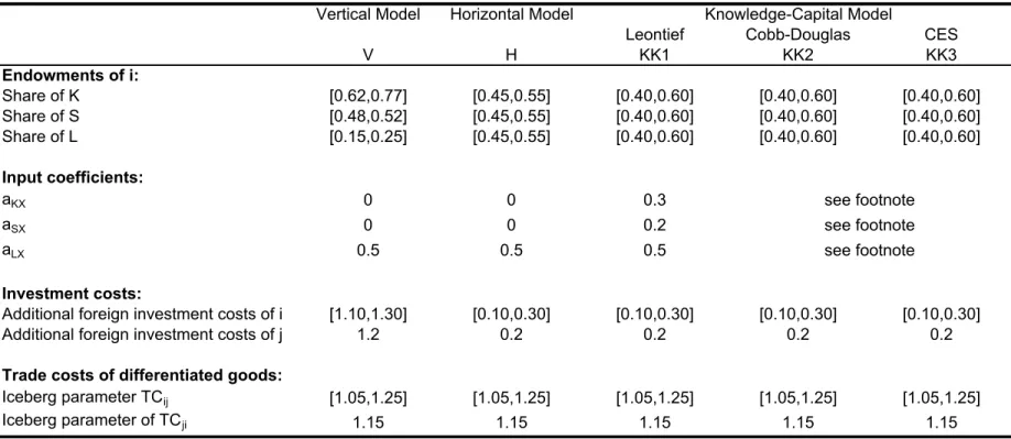
We simulate various versions of our model. In so doing, we stick to the notion that both the model of vertical MNEs (Helpman, 1984, Helpman and Krugman, 1985) and that of horizontal MNEs (Markusen, 1984, Markusen and Venables, 1998, 2000) are restricted variants of the knowledge-capital model, where both types of firms may endogenously arise (Carr, Markusen and Maskus, 2001, Markusen, 2002). However, a pure horizontal model and a pure vertical one are also calibrated. Altogether, we set up five different models: a KK-model based on a Leontief technology in the X-sector; a KK-KK-model based on a Cobb-Douglas technology in the X-sector; a KK-model based on aCES-technology in the X-sector assuming a more realistic technical rate of substitution of between 0 and 1 (see Sharma, 2002; we choose a relatively low value of 0.1); a horizontal Leontief-based model; and a vertical Leontief-based model.26

In sum, we compute the equilibrium Grubel-Lloyd index for 21×21×21=9261 cells of the factor cube and 5 different levels of country i’s fixed FDI-related investment costs (country

j’s investment costs are always set at a fixed value). This gives 46305 equilibrium values for each model without trade cost differences. Additionally, we simulate a set of equilibria, where trade costs for exports from country i to j amount to 5%-25%, leaving those of exports from j

to i always at 15%. Where countries differ in trade costs, there are a further 4×9261=37044 equilibrium values. Pooling the two sets of equilibria allows us to search for the preferred specification in the empirical analysis, accounting for the same variables. Altogether, there are 83349 observations for each model. Specifically, we estimate the following models:

(

)

(

)

(

(

)

)

0 1 2 2 2 3 4 5 6 ln( ) ln 1 / / ln | / - / | ln | ( / - / ) | ln | (1 ) - (1 ) | ln C ij i j i i j j i j i i j j i i j j i j ij ji ij LGLI GDP GDP GDP GDP GDP GDP GDP GDP K L K L S L S L INVC INVC TC TC α α α α α α α = + +   + _ − + − + _   + + + + + + − +ζ (M1)

(

)

(

)

(

)

2 2 0 1 2 3 2 2 2 4 5 6 7 ln( ) ( - ) ( / - / ) ( / - / ) + ( - ) ( / - / ) ln 0.5 1 0.5 1 ln 0.5 0.5 C ij i j i j i i j j i i j j i j i i j j i j ij ji ij LGLI GDP GDP GDP GDP K L K L S L S L GDP GDP S L S L INVC INVC TC TC β β β β β β β β ζ = + + + + + ×   + _ + + + _+ + + (M2)

(

)

0 1 2 3 4 5 6 max{ln ,ln } min{ln ,ln } ln | ( / - / ) | ln | ( / - / ) | ln | (1 ) - (1 ) | ln 0.5 0.5 C ij i j i j i i j j i i j j i j ij ji ij LGLI GDP GDP GDP GDP K L K L S L S L INVC INVC TC TC χ χ χ χ χ χ χ ζ = + + + + + + + + + + (M3) 0 1 2 3 4 5 6 7 8 max{ln ,ln } min{ln ,ln } max{ln( / ),ln( / )} min{ln( / ),ln( / )} max{ln( / ),ln( / )} min{ln( / ),ln( / )} max{ln(1 ),ln(1 )} min{ln C ij i j i j i i j j i i j j i i j j i i j j i j LGLI GDP GDP GDP GDP K L K L K L K L S L S L S L S L INVC INVC δ δ δ δ δ δ δ δ δ = + + + + + + + + + +

( ) ( )

{

}

{

( ) ( )

}

9 10 (1 ),ln(1 )} + max ln ,ln + min ln ,ln + i j ij ji ij ji ij INVC INVC TC TC TC TC δ δ ζ + + (M4) C ij

LGLI denotes the logistically transformed, corrected Grubel-Lloyd index, INVC refers to investment costs and g γ of our theoretical analysis, respectively, and TC (TC ) is a measure of transport costs for shipping differentiated goods from country (i) to country i

( ).

ji ij

j

j 27

M1 is closest to Helpman (1987) but with the addition of differences in investment costs; M2 is closest to Markusen and Maskus (2001), extended by the squared difference in capital-labour ratios; M3 is in the spirit of Hummels and Levinsohn (1995), with the addition of absolute difference in skilled-to-unskilled labour ratios; and M4 extends their idea of allowing for asymmetric influences between maximum and minimum levels of all variables.

27 _{In terms of our analytical model,}

(

_{2 1/}

)

ij = − tij

TC gives the volume of production that is necessary if one unit of the differentiated good is consumed abroad.

Running those four specifications results in the following adjusted R2 figures:

Horizontal Vertical KK-Leontief KK-CD KK-CES

M1 0.0115 0.2345 0.1469 0.0082 0.0568

M2 0.0685 0.3507 0.1419 0.0569 0.0624

M3 0.0113 0.3157 0.1147 0.0113 0.0557

M4 0.1056 0.5085 0.1563 0.0933 0.0880

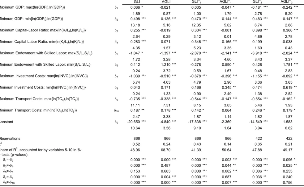
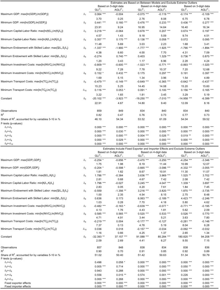
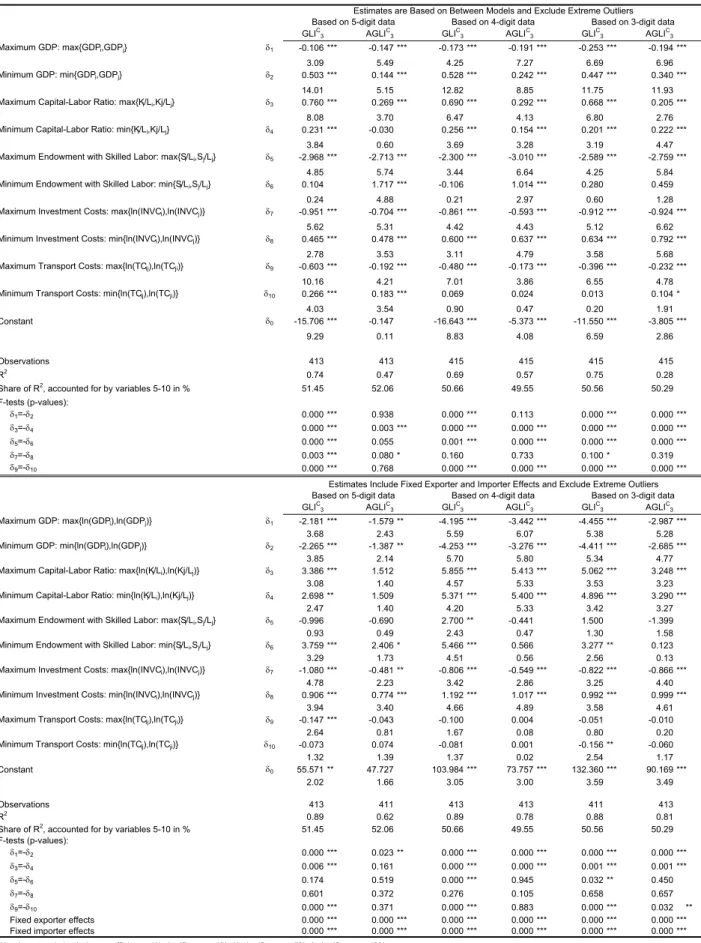
With the exception of the vertical model, the reported R2 figures are relatively low, reflecting the high degree of non-linearity in these type of models. Of course, omitting the skills and friction variables in M1 or M3 would lead to specifications which are closer to Helpman (1987) and Hummels and Levisohn (1995), but inferior in terms of explanatory power. Similarly, omitting the capital terms in M2 would render the model closer to Markusen and Maskus (2001) but also inferior. On the other hand, using the maximum and minimum values of both trade and investment frictions in every model reduces the difference in adjusted R2 figures, but without changing their ranking. Empirically, the repeated observation of each country in a bilateral setting and the use of country-specific effects improve the fit.

As can be seen, M4 consistently outperforms M1-M3. With regard to the estimated coefficients of M4, two weak hypotheses can be formulated. First, δ1<0 and δ2<0 are more

likely if horizontal MNEs dominate28 Note that horizontal MNE activity is market-seeking, i.e. growing with market size, and crowds out two-way trade in differentiated goods, explaining the expected sign of δ₁. The result δ₂<0 is due to the non-linearities, caused by complementary slackness. Suppose that there is initially a very small country, so that it does not pay to set up horizontal MNEs. In such an economy, intra-industry trade accounts for a large share of trade. As we reallocate absolute factor endowments to this economy, at some point it is profitable to establish horizontal MNEs and intra-industry trade falls. As countries become more similar, the IIT share rises again. In our case, the effect induced by the complementary slackness dominates and δ₂ is negative. However, δ1<0 indicates that

similarity in size is important and tends to increase the IIT share if δ₁ dominates δ₂. Vertical MNEs tend to foster intra-industry trade but they are stimulated by dissimilarities in country size, in line with our analytical investigation (see Fact 1).

Second, for similar reasons the maximum investment cost coefficient δ7 is negative with

two-way horizontal FDI (see Result 2). Hence, the share of IIT tends to rise with the similarity in investment costs. Finally, the difference between the maximum value and the corresponding minimum value of the skilled to unskilled labour coefficients (δ₅ −δ₆) tends by and large to be negative, which supports the common finding that IIT is higher between economies with more similar factor endowments (Helpman, 1987, Bergstrand, 1990, Hummels and Levinsohn, 1995). With regard to the impact of capital-labour ratios, remember that setting up horizontal MNEs is the most capital intensive activity. Horizontal MNEs seem empirically important and note that the share of intra-industry trade in total imbalance-corrected trade tends to rise if horizontal FDI increases. However, with co-existing horizontal and vertical or only vertical FDI the impact of capital-labour ratios gets less clear-cut.

2.4 Summary of the theoretical hypotheses for the Grubel-Lloyd index

From our analytical investigation we obtain the following hypotheses. With horizontal MNEs an increase in investment costs g tends to reduce GL , if g increases in the L-abundant country. In contrast, if g rises in the country with scarce L supply, increases. With vertical MNEs, an increase in FDI-costs tends to reduce the intra-industry trade share if in the country that hosts the vertical multinational firms factor L is relatively scarce (so that this economy is a net exporter of the differentiated good. In contrast, if the country that hosts the vertical multinationals is relatively L-abundant and, therefore, is a net importer of the differentiated good, GL tends to be positively (non-negatively) affected by an increase in FDI-costs. The simulation exercise generates two additional hypotheses. First, the country size (δ C I C GLI C I

1,δ2) coefficients are more likely negative, if horizontal MNEs dominate at a reasonable

value of the elasticity of substitution (see Feenstra, 1994, for detailed empirical evidence). Second, intra-industry trade is by and large higher between economies with more similar skilled-to-unskilled labour endowments and investment costs with two-way horizontal FDI, but less likely the more important vertical FDI is.

3 Empirical

analysis

3.1 The Grubel-Lloyd index in the empirical trade literature

Grubel and Lloyd (1971) had in mind a model with zero transport costs and no multinational firms. Both transport costs and MNE activity are now understood as essential characteristics

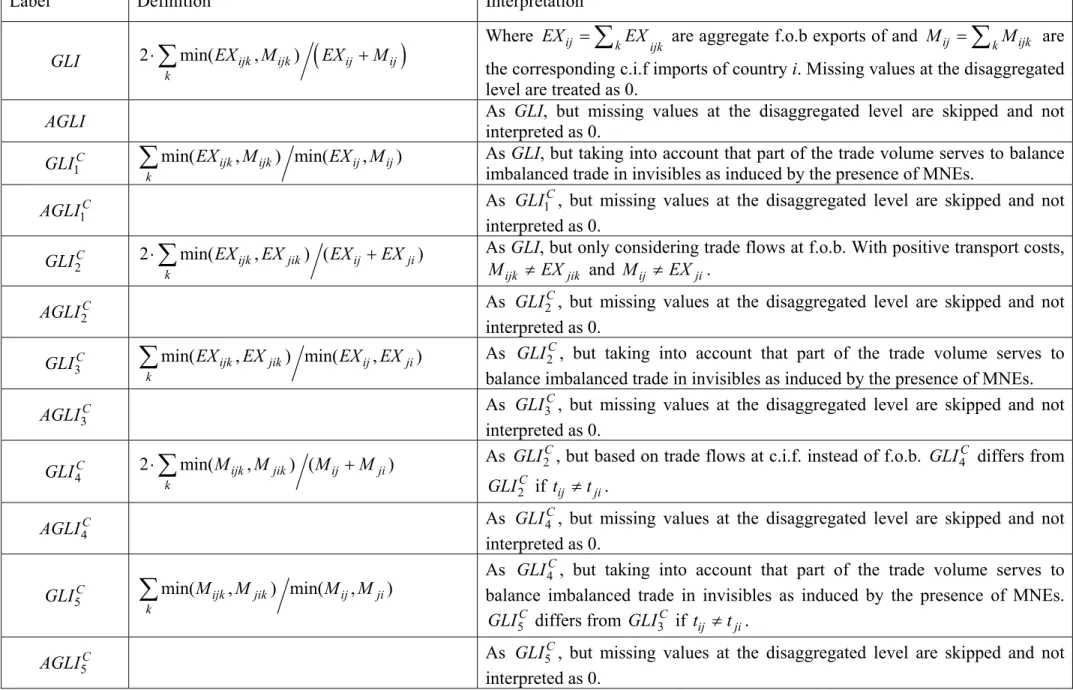
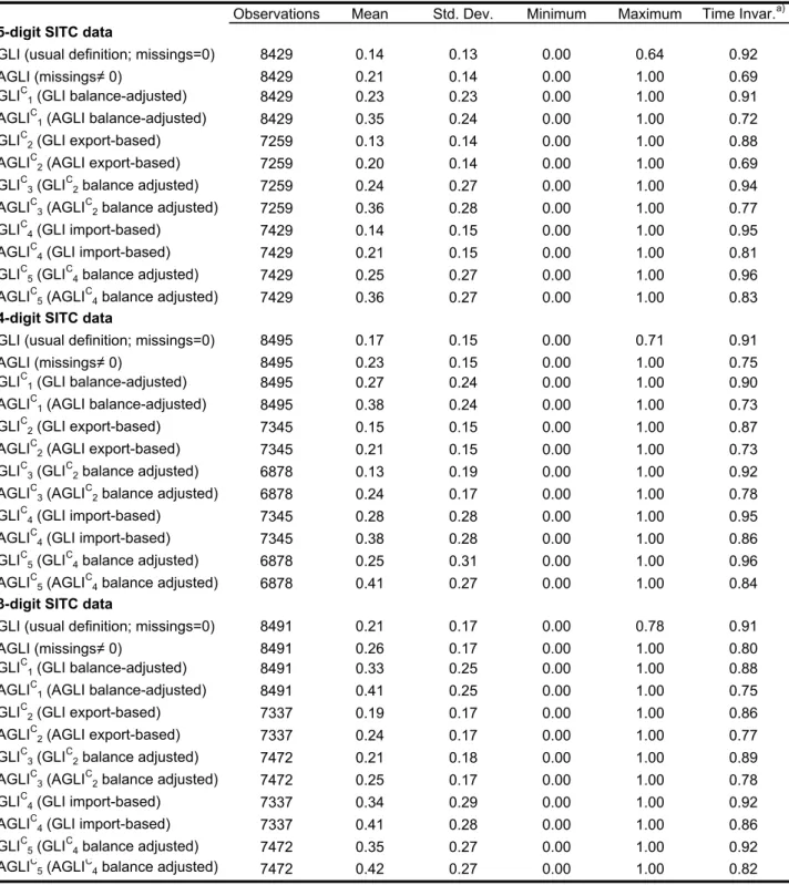
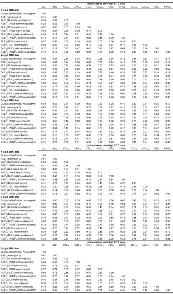
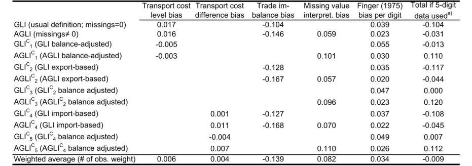
of international exchange. However, their consequences for the measurement (and determinants) of intra-industry trade shares has to the best of our knowledge not yet been rigorously studied. Below, we provide several alternative versions of the Grubel-Lloyd index, which can cope with both transport costs and MNE activity. (We also explicitly discuss issues such as the interpretation of missing values in the disaggregated trade data, the index is based on.) Table 1 summarizes.29

> Table 1 <

It seems sensible to start with the original formulation of the index as also applied in Helpman (1987), Hummels and Levinsohn (1995), or Markusen and Maskus (2001). In the case of a two-country, new trade theory model with zero transport costs and no MNE activity,

.

1C 2C 3C 4C C

GLI ≡GLI ≡GLI ≡GLI ≡GLI ≡GLI₅

With multinational firms, trade is not necessarily (or even likely to be) balanced. To see the relevance of this, consider the simple thought experiment of two one-sector economies with MNEs. Not accounting for income flows due to repatriated profits leads to a downward bias of the Grubel-Lloyd index, i.e. GLI GLI− ₁C <0, GLI₂C −GLI₃C <0

3C

GLI I₅C

and GL ,

which we refer to as the trade imbalance bias in absolute terms (in contrast to the relative measure of this bias, SHI, calculated above).

4C 5C 0

I −GLI <

30 _{Hence, there remain three candidates for}

measuring the intra-industry trade share: GL , and GL which differ if transport costs are positive.

1C

I

Now consider the impact of transport costs, but stick for the moment to the usual assumption

that . In this case, . Note that , because the

denominator of is higher than the denominator of GLI due to transport costs included

ij ji

t =t _GLIC _GLIC _GLIC

5 3 1 ≠ ≡ GLI1C ≠GLI3C C GLI_{1 3}C

29 _{The Grubel-Lloyd indices in Table 1 measure bilateral intra-industry trade in a multi-country world. Hence,}

are country i’s exports to and

ij

EX IM_ij are country i’s imports from country j. Index k indicates different industries.

30 _{The arguments in Greenaway et al. (2001) are related to our arguments. Bergstrand (1983) correctly points out}

that bilateral trade tends to be unbalanced also in a multilateral setting without MNEs. Our approach also covers this phenomenon.