1
Nonlinear parametric modelling to study how soil properties affect
1crop yields and NDVI
2Rebecca Whettona, Yifan Zhaob, Sameh Shaddadc, Abdul M Mouazena,d* 3
a Cranfield Soil and AgriFood Institute, Cranfield University, Bedfordshire MK43 0AL, UK.
4
bThrough-life Engineering Services Institute, Cranfield University, Bedfordshire MK43 0AL, UK
5
c Soil Science Department, Faculty of Agriculture, Zagazig University 44511- Zagazig, Egypt
6
d Precision Soil & Crop Engineering Group, Ghent University, Coupure 653, 9000 Gent, Belgium
7
* E-mail of corresponding author: [email protected]
8
Abstract 9
This paper explores the use of a novel nonlinear parametric modelling technique based on a Volterra Non-linear 10
Regressive with eXogenous inputs (VNRX) method to quantify the individual, interaction and overall 11
contributions of six soil properties on crop yield and normalised difference vegetation index (NDVI). The 12
proposed technique has been applied on high sampling resolution data of soil total nitrogen (TN) in %, total 13
carbon (TC) in %, potassium (K) in cmol kg-1, pH, phosphorous (P) in mg kg-1 and moisture content (MC) in %, 14
collected with an on-line visible and near infrared (VIS-NIR) spectroscopy sensor from a 18 ha field in 15
Bedfordshire, UK over 2013 (wheat) and 2015 (spring barley) cropping seasons. The on-line soil data were first 16
subjected to a raster analysis to produce a common 5 m by 5 m grid, before they were used as inputs into the 17
VNRX model, whereas crop yield and NDVI represented system outputs. Results revealed that the largest 18
contributions commonly observed for both yield and NDVI were from K, P and TC. The highest sum of the 19
error reduction ratio (SERR) of 48.59% was calculated with the VNRX model for NDVI, which was in line with 20
the highest correlation coefficient (r)of 0.71 found between measured and predicted NDVI. However, on-line 21
measured soil properties led to larger contributions to early measured NDVI than to a late measurement in the 22
growing season. The performance of the VNRX model was better for NDVI than for yield, which was attributed 23
to the exclusion of the influence of crop diseases, appearing at late growing stages. It was recommended to 24
adopt the VNRX method for quantifying the contribution of on-line collected soil properties to crop NDVI and 25
yield. However, it is important for future work to include additional soil properties and to account for other 26
factors affecting crop growth and yield, to improve the performance of the VNRX model. 27
Keywords
28
Yield limiting factors; proximal soil sensing; nonlinear parametric modelling; VNRX. 29
Computers and Electronics in Agriculture, Volume 138, 1 June 2017, Pages 127-136 DOI:10.1016/j.compag.2017.04.016
Published by Elsevier. This is the Author Accepted Manuscript issued with:Creative Commons Attribution Non-Commercial No Derivatives License (CC:BY:NC:ND 4.0). The final published version (version of record) is available online at DOI:10.1016/j.compag.2017.04.016. Please refer to any applicable publisher terms of use.
2
1. Introduction
30
Increasing crop yields requires the precision management of external farm resources (i.e., 31
agrochemicals and fertilisers), which will help reduce input costs and detrimental 32
environmental impacts. Precision management of farm resources requires an understanding 33
and quantification of factors that limit crop yields, which is a research question yet to be 34
comprehensively answered. This currently prohibits precision management of farm resources 35
to be a routine activity. However, precision management of farm resources to correct existing 36
yield limiting factors require high sampling resolution data of variables impacting crop 37
growth and yield, which can then be incorporated within an analytical system. To realise this, 38
robust and reliable sensing platforms for soil and crop are needed. Due to the complexity and 39
high spatial variability of soils, the application of proximal soil sensors is still under active 40
research. Kuang et al. (2012) argue that the most favourable methods for on-line 41
measurement of key soil properties are visible and near infrared (VIS-NIR) spectroscopy and 42
electrochemical methods. The former is based on diffuse reflectance light collected from a 43
soil surface subjected to an external light source, whereas the latter uses ion selective 44
elements to produce a voltage output in a solution in response to the activity of the selected 45
ion (e.g., hydrogen, nitrate). Whilst VIS-NIR is most appropriate to soil properties have direct 46
spectral responses in the NIR spectral range, i.e., organic carbon (OC), moisture content 47
(MC), clay and clay mineralogy (Stenberg et al., 2010), electrochemical methods are capable 48
of quantifying mobile elements i.e., nutrients, mineral nitrogen, or pH (Adamchuk et al., 49
1999). Since a soil solution is required for electrochemical sensors, their on-line use is 50
impeded. Although on-line VIS-NIR spectroscopy sensors are capable of collecting high 51
sampling resolution data (e.g., >500 samples per ha), they are limited to few research groups 52
(Christy, 2008; Shibusawa, et al. 2001; Mouazen et al., 2006a). Once key soil properties 53
needed in the analytical system are successfully collated using an on-line sensor, information 54
3
about crop growth (i.e., normalised difference vegetation index (NDVI) or leaf area index 55
(LAI)) can be obtained at high sampling resolution by means of earth observation utilising 56
satellite, airborne, drones or proximal crop sensing platforms. 57
Previous research has often assumed that the relationship between crop yield and growth 58
limiting factors is linear or approximately linear, which could be untrue for typically complex 59
agriculture systems. Mitscherlich (1909) proposed a model that simulates crop response to 60
growth factors increase. The model assumes that yield potential is constant, and isn’t affected 61
by other factors that limit actual yields under field conditions; a further assumption that may 62
be false in complex agricultural systems. To reveal and characterise information hidden 63
within this complex system, a non-linear modelling approach is required to describe the 64
dependence among soil properties, NDVI and crop yield. Through these means, yield limiting 65
soil properties can be quantified. 66
Nonlinear methods include, among others, non-linear regression analyses and machine 67
learning. The Nonlinear Auto-Regressive Moving Average Model with eXogenous inputs 68
(NARMAX) is a parametric modelling method introduced by Billings et al. (1989). It is a 69
popular class of nonlinear system identification methods for a complex system, which 70
represents a typical input-output system with an unknown inner structure. Compared to 71
machine learning methods, an advantage of NARMAX is transparency. This means it can be 72
written down and easily understood and interpreted, related to known and existing models, as 73
well as being coupled with frequency domain or statistical analyses. These characteristics are 74
attractive for studying brain climatic change and agriculture systems that are typical input-75
output systems with unknown inner structures. A Volterra Nonlinear Regressive with 76
eXogenous inputs (VNRX) is a special case of NARMAX that has more recently been 77
introduced. Although VNRX has had successful applications in brain signal analysis 78
(Sarrigiannis et al., 2014; Zhao et al., 2012), climate change (Bigg et al., 2014; Zhao et al., 79
4
2016) and non-destructive tests (Zhao et al., 2017), its application in agriculture is novel due 80
to its capability to reveal hidden nonlinear information while other modelling methods cannot. 81
To our best knowledge no literature about the use of the VNRX model to predict NDVI and 82
crop yield based on on-line measured soil properties is available. This is important to 83
investigate, since on-line soil sensors provide high sampling resolution data (>500 sample per 84
ha), to enable accounting for variability over small spatial scales (e.g., few meters), which 85
cannot be efficiently achieved using traditional methods of soil sampling and laboratory 86
analyses that are tedious, time consuming and costly. 87
This study’s aim is to implement a novel parametric VNRX model to quantify individual, 88
interaction and collective contribution of six soil properties (i.e., TN, total carbon (TC), 89
potassium (K), pH, phosphorous (P), and MC) on crop yield and NDVI. Soil data has been 90
collected at a high sampling resolution with an on-line VIS-NIRspectroscopy sensor. 91
2. Materials and methods
92
2.1 Study site and data collection 93
The study site is located on commercial farmland in Wilstead, Bedfordshire, United Kingdom 94
at coordinates 52°6’0.00”W latitude and 0°26’42.00”N longitude. The field is approximately 95
18 ha in area, with an average annual rainfall of 598 mm. The farms crop rotation consists of 96
barley, wheat and oil seed rape. The representative soil texture across the field to a depth of 97
0.20 m is non-homogeneous, including three textures of sandy loam, loam and sandy clay 98
loam in accordance with the United States Department of Agriculture (USDA) texture 99
classification system (Soil Survey Staff,1999). Wheat and spring barley were cultivated over 100
the experiment timescale during the 2013 and 2015 cropping seasons, respectively. Soil 101
properties, yield and NDVI data were collected using an on-line VIS-NIR spectroscopy 102
sensor (Mouazen, 2006), on-board yield sensor from the farmer’s combine harvester (New 103
Holland, CX8070 model), and a Crop Circle sensor (Crop Circle ACS 470, Holland Scientific, 104
5
Lincoln, NE USA), respectively. Wheat NDVI was measured in the booting (growth stage43) 105
and heading (growth stage 52) stages, in May and June 2013, respectively. Spring barley 106
NDVI was measured during the stem extension (growth stage37) and booting (growth stage 107
43) stages in April and May 2015, respectively. The growing stages are determined in 108
accordance with Zadok’s decimal growth scale (Zadoks et al., 1974). 109
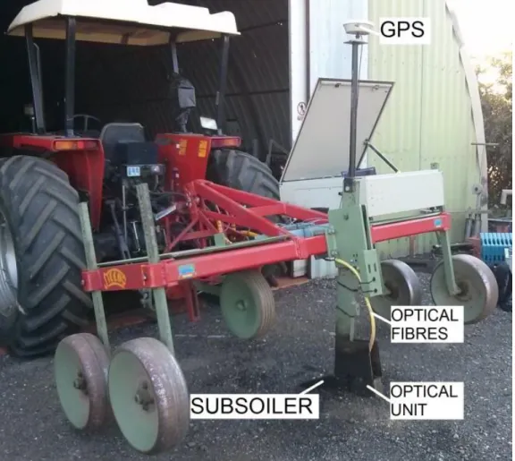
The on-line VIS-NIRsoil sensor (Mouazen, 2006b) (Fig.1) consisted of an AgroSpec mobile, 110
VIS-NIR spectrophotometer (tec5 Technology for Spectroscopy, Germany), with a 111
measurement range of 305-2200 nm. It has a differential global positioning system (DGPS) 112
(EZ-Guide 250, Trimble, USA) to record the position of the on-line measured spectra with 113
sub-metre accuracy. An optical probe fitted behind a subsoiler collected diffuse reflected 114
Fig. 1. The tractor mounted on-line visible and near infrared (VIS-NIR) spectroscopy sensor (Mouazen, 2006b).
6
spectra from the bottom of a smooth soil trench formed by the subsoiler. A 20 W halogen 115
lamp supplied by a tractor battery illuminated the base of the trench with artificial light. A 116
semi-rugged laptop was used for data logging and communication to the instrument. 117
On-line soil measurements were carried out in September 2012 and 2014, following crop 118
harvest, using the method reported in Mouazen et al. (2005). These measurements will be 119
referred to as 2013 and 2015 soil measurements, respectively, throughout the manuscript. The 120
on-line sensor produced measurementtransects that were 6 cm wide, 15 cm deep, and were 121
distanced 15 m apart. The spectral measurements were collected with an average forward 122
speed of 2 km h-1.Both on-line measurement and collection of soil samples were performed 123
prior to seed drilling (October in 2012 for wheat and February 2015 for spring barley) and 124
fertilisation (April to June in 2013 and 2015). Soil property changes during winter between 125
on-line measurement and next growing season are minimal, except for MC. However, the 126
spatial distribution of MC in a topographically uniform field like the study site may be 127
similar to the spatial distribution of clay (Mouazen et al., 2014), suggesting that the general 128
spatial pattern of MC would not significantly change from year to year. Only nitrogen 129
fertiliser was homogeneously applied in the 2013 and 2015 cropping seasons, whereas no K 130
or P fertilisers were applied. 131
2.2 Laboratory analysis and development of calibration models of soil properties 132
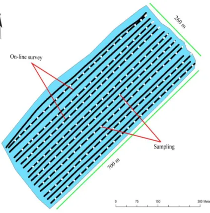
Ten soil samples per hectare (183 samples per 18 ha field area) based on a 30 by 30 m grid 133
(Fig. 2) were collected during the on-line measurement in 2012 from the bottom of the 134
subsoiler trenches. Sampling positions were recorded with a DGPS (Shaddad et al., 2016). 135
Approximately 700 g representing each soil sample was prepared as a composite of soil 136
collected over a 1.5 m travel distance at about 0.15 m depth. Soil samples were placed into 137
tightly sealed plastic bags to hold field moisture, and kept refrigerated at 4 ºC, until 138
7
laboratory analyses to determine TN, TC, K, pH, P and MC. These analyses were based on 139
the following procedures: 140
TN and TC were determined with CHN 628 elemental analysis by combustion (LECO, 141
USA) (British Standard Institute, 1995). 142
Exchangeable K was determined using an atomic absorption spectrometer (AA 143
analyst 200 Perkin Elmer Instruments, Shelton, Connecticut, USA). 144
pH was measured using a glass electrode in a 1:5 (volume fraction) suspension of soil 145
in distilled water (British Standard Institute, 1998). 146
Extractable P was obtained in sodium hydrogen carbonate solution according to ISO 147
11263:1994 (Olsen et al., 1954) and was determined by colorimetric approach using 148
UV-VIS-NIR spectrophotometer (Murphy and Riley, 1962). 149
Gravimetric MC was measured with oven drying at 105 ºC for 24 h (British Standards 150
Institute, 2007). 151
8
Results of laboratory analyses and spectral measurements were pooled together in one matrix. 152
The 183 soil samples were randomly split into calibration (70% of samples) and validation 153
(30%) sets. The calibration set was subjected to partial least squares regression (PLSR) 154
analysis to establish calibration models for the studied soil properties using Unscrambler 155
V9.8 software (Camo Software, Norway) (Shaddad et al., 2016). PLSR models were 156
validated using the 30% validation samples that were not included in the PLSR calibration 157
stage. Models were then used to predict the six soil properties using the on-line collected soil 158
spectra in September 2012 and 2014. The accuracy of these models are assessed by means of 159
the ratio of prediction deviation (RPD), which equals the standard deviation of laboratory 160
measured values divided by root mean square error of prediction (RMSEP). The following 161
RPD classes proposed by Viscarra Rossel et al. (2006) were adopted in this study: RPD < 1.0 162
indicates very poor model predictions and their use is not recommended; an RPD between 1.0 163
and 1.4 indicates poor model predictions, where only high and low values are distinguishable; 164
an RPD between 1.4 and 1.8 indicates fair model predictions, which may be used for 165
assessment and correlation; an RPD between 1.8 and 2.0 indicates good model predictions, 166
where quantitative predictions are possible; an RPD between 2.0 and 2.5 indicates very good 167
quantitative model predictions; and an RPD > 2.5 indicates excellent model predictions. 168
2.3 Data processing 169
Data processing begun with kriging of the on-line VIS-NIR predicted soil properties and 170
measured crop NDVI and yield. Kriged data layers were converted into a common 5 m2 raster 171
grid in ArcGIS (Esri, USA) to aid data fusion (Frogbrook and Oliver, 2007). The 5 m2 raster 172
grid was converted into a common grid of points that represented the value at the midpoint of 173
each raster pixel. These steps ensured that all layers consisted of common sets of 5 m2 grid 174
points, essential for running the VNRX analysis. This method allowed fusion of data from a 175
diverse range of soil and crop property (e.g., NDVI, Yield, etc.) surveys, measured at 176
9
different resolutions (Khosla et al., 2008). However, it is worth noting that converting data 177
from 5 m2 raster squares to point locations introduced unavoidable errors to the data’s spatial 178
distribution. Finally, the different soil and crop layers of 5 m2 grid were subjected to the 179
VNRX non-linear parametric modelling, which is explained further in the following section. 180
2.4 Non-linear parametric modelling 181
The VNRX model, also known as nonlinear finite impulse response (NFIR) model, is used in 182
this paper to represent a multi-inputs and single-output system. The model can be expressed 183
as: 184
𝑦(𝑘) = 𝑓(𝑢1[𝑘−1], 𝑢2[𝑘−1], … , 𝑢𝑅[𝑘−1]) + 𝜀(𝑘) (1)
185
where 𝑘(𝑘 = 1,2, . . ) is a time index, 𝑅 is the number of system inputs, 𝑓 is some unknown 186
linear or non-linear mapping, which links the system output 𝑦 to the system 187
inputs 𝑢1, 𝑢2, … , 𝑢𝑅 and 𝜀(𝑘) denotes the model residual. The symbol 𝑢𝑖[𝑘−1](𝑖 = 1,2, … , 𝑅) 188
denotes the past information of the input 𝑢𝑖, which can be expanded as:
189
𝑢𝑖[𝑘−1] = ⋃𝑛𝑗=0𝑖 𝑢𝑖(𝑘 − 𝑗) (2)
190
where 𝑛𝑖 is the maximum temporal lag to be considered for the input 𝑢𝑖. 191
The Volterra series is a model for nonlinear behaviour that has similarities to the Taylor 192
series. However, it differs from the Taylor series in its ability to capture 'memory' effects. 193
The Taylor series can be used to approximate the response of a nonlinear system to given 194
inputs if the output of this system depends strictly on the inputs at that particular time. In the 195
Volterra series the output of the nonlinear system depends on the input to the system at all 196
previous times. This provides the ability to capture the 'memory' effect of devices like 197
capacitors and inductors (Tashev, 2009). 198
10
A commonly employed model type to specify the function f in Eq. (1) is a polynomial 199
function (Chen and Billings, 1989; Wei et al., 2004), which can be expressed as: 200
𝑦 = 𝜃0 + ∑𝑁𝑚=1𝜃𝑚∅𝑚+ 𝜀 (3) 201
where ∅𝑚 is the 𝑚𝑡ℎ model term generated from all input vectors, 𝜃𝑚 is the corresponding 202
unknown parameters, and 𝑁 is the total number of potential model terms. It is worth noting 203
that ∅𝑚 is, in general, non-linear. Considering a system with two inputs 𝑢1 and 𝑢2, a second
204
order polynomial function can be written as: 205
𝑦 = 𝜃0+ 𝜃1𝑢1+ 𝜃2𝑢2+ 𝜃3𝑢12+ 𝜃4𝑢22+ 𝜃5𝑢1𝑢2+ 𝜀 (4) 206
The next step is to estimate the parameters 𝜃𝑚(𝑚 = 0,1, … ,5) based on the
207
observations {𝑦, 𝑢1, 𝑢2}. The procedure begins by determining the structure, or the important 208
model terms, using the orthogonal least squares (OLS) estimation procedures. It determines 209
which dynamics and nonlinear terms should be included in the model by computing the 210
contribution that each potential model term makes to the variation of the system output. The 211
model is to be built up term by term in a manner that exposes the significance of each new 212
term that is added. Once the structure of the model has been determined, the unknown 213
parameters can be estimated, and the procedure of model validation can ensure the model is 214
adequate. In this paper, a routine called adaptive-forward-orthogonal least squares (AFOLS) 215
was employed, not only to determine the model structure, but also to estimate unknown 216
parameters. The forward model selection scheme adopted consisted of a greedy optimisation 217
algorithm that progressively includes additional terms into the model, starting from an empty 218
structure, on the basis of the error reduction ratio (ERR) criterion (Cantelmo and Piroddi, 219
2010). It is a well-tested strategy for parsimonious modelling of data due to its effectiveness 220
and merit to reduce ill conditioning and overfitting problems (Zhao et al., 2012). 221
11
The on-line measured soil properties (i.e., pH, MC, TN, P, K and TC) were normalised by 222
removing the mean of each property, after which they were used as inputs to the VNRX 223
model, whereas the model output was mean normalised crop yield and NDVI. The analysis 224
also included the interaction between pairs of soil properties and their contribution to crop 225
yield and NDVI. The aim was to investigate the contribution of each soil property and their 226
pairwise interaction on crop NDVI and yield on one hand and to understand how the 227
contribution varied amongst different cropping seasons on the other hand. To calculate the 228
contribution of soil properties on yield, the NVRX analysis was carried out once in each 229
cropping season in 2013 and 2015. However, for NDVI, the NVRX model was run twice per 230
cropping season (e.g., May and June in 2013, and April and May in 2015). The VNRX 231
modelling was carried out utilising Microsoft visual studio code written with C++ 232
programming language. 233
Finally, the performance of the VNRX model in the prediction of NDVI and yield was 234
evaluated by means of the of error reduction ratio (ERR) for each selected term calculated 235
from AFOLS that measures the percentage this term contributes to the system output. Values 236
of ERR always range between 0% and 100%. A higher ERR represents a greater dependence 237
between this term and the output. Therefore, it is an important index for indicating the 238
importance of each term to the output. To calculate the contribution of each input variable to 239
the output, the sum of ERR values of all selected terms, denoted by 𝑆𝐸𝑅𝑅, and calculated by 240
𝑆𝐸𝑅𝑅 = ∑𝑁𝑖=1[𝑒𝑟𝑟]𝑖 (5) 241
was used to describe the percentage explained by the identified model to the system output, 242
where 𝑁 denotes the number of the selected terms. If the considered inputs can fully explain 243
the variation of system output, the value of 𝑆𝐸𝑅𝑅 is equal to 100%. It is an indicator of 244
model performance and uncertainty. The contribution of the 𝑖𝑡ℎ input variable to the variation 245
12
of the system output, denoted as 𝐸𝑅𝑅𝐶𝑖, is defined as the sum of ERR values of the terms 246
that include this input variable. Because some selected terms may involve more than one 247
input variable due to nonlinearity, the sum of 𝐸𝑅𝑅𝐶𝑖 for all input variables can be greater 248
than 𝑆𝐸𝑅𝑅. To overcome this problem, the value of 𝐸𝑅𝑅𝐶𝑖 is used, which can be written as: 249
𝐸𝑅𝑅𝐶𝑖 =
∑𝑁𝑗=1([𝑒𝑟𝑟]𝑗|𝑢𝑖∈∅𝑗)
∑𝑟𝑝=1∑𝑁𝑗=1([𝑒𝑟𝑟]𝑗|𝑢𝑝∈∅𝑗)×𝑆𝐸𝑅𝑅 (6)
250
The value of 𝐸𝑅𝑅𝐶𝑖 should be always between 0% and 100%. 251
2.5 Mapping 252
Similar spatial distributions of measured versus predicted NDVI and yield were evaluated by 253
comparing the corresponding maps. Maps were produced through interpolation with an 254
inverse distance weighing (IDW) method, using ArcGIS software (ESRI, USA). The 255
interpolation grid size of all maps had a radius of 12.5 m and a power of 2. The map cell size 256
was 2.5 m2 with 254 rows and 282 columns. Similarity between maps was assessed by visual 257
comparison. In addition, Pearson’s correlation (r) coefficient was calculated between each 258
pair of data sets used to produce maps. 259
3. Results and discussion 260
3.1 Accuracy of on-line measured soil properties 261
The best independent validation of PLSR calibration models using on-line spectra (Table 1) 262
is obtained for pH and TN with RPD values of 2.06 (very good prediction) and 1.85 (good 263
model prediction), and RMSEP values of 0.434 and 0.013 (%), respectively (Shaddad, 2013). 264
These results are better than those reported by Mouazen et al. (2007). Although both TC and 265
MC have direct spectral responses in the NIR spectral range, they have not resulted in the 266
best prediction accuracy in this study (Table 1). RPD values of P, TC and MC are rather 267
small with values of 1.77, 1.50 and 1.49, respectively, which are classified as fair model 268
13
predictions. The lowest RPD value of 1.31 is calculated for K, indicating poor prediction 269
accuracy (Viscarra Rossel et al., 2006). 270
271
3.2 Influences of soil properties on yield 272
Statistics for on-line measured soil properties used as input in the VNRX model are provided 273
in Table 2. Observed ranges (e.g., minimum and maximum values) are different between 274
2013 and 2015, which can be attributed to farm practices (e.g., fertilisation) and different 275
weather conditions affecting soil MC in particular. 276
277
Table 1: Range of on-line measured soil pH, phosphorous (P), total nitrogen (TN), total carbon (TC), moisture content (MC) and exchangeable potassium (K) used in the Volterra Nonlinear Regressive with eXogenous inputs (VNRX) models.
Year Range pH P (mg kg-1) TN (%) TC (%) MC (%) K (cmol kg-1)
2013 Min 5.31 20.33 0.11 1.46 11.98 0.18
Max 7.83 56.21 0.18 2.40 17.41 0.31
2015 Min 5.87 26.83 0.05 0.92 4.53 0.22
Max 6.44 43.34 0.16 1.81 9.79 0.47
Table 2: Validation of partial least squares regression (PLSR) models to predict soil pH, phosphorous (P), total nitrogen (TN), total carbon (TC), moisture content (MC) and exchangeable potassium (K) using on-line collected spectra of the prediction set.
Soil properties Statistics pH P (mg kg-1) TN (%) TC (%) MC (%) K (cmol kg-1) Sample no 48 23 22 24 45 24 Min 5.16 4.80 0.11 1.30 13.41 0.12 Max 8.17 50.00 0.20 2.46 24.28 0.40 Mean 6.46 22.50 0.15 1.79 18.03 0.23 SD 0.90 15.23 0.02 0.28 2.16 0.08 RMSEP* 0.43 8.61 0.01 0.18 1.45 0.06 R2 0.73 0.69 0.72 0.57 0.56 0.44 RPD 2.06 1.77 1.85 1.50 1.49 1.31 Model quality** A B A B B C
*RMSEP: Root mean square error of prediction; **Model quality is categorized according to Viscarra Rossel et
14
Based on Eq. (3), the polynomial model to express the relationship between the six input soil 278
variables and the output NDVI and yield is of quadratic terms, written as: 279
𝑦 = 𝜃0+ ∑6𝑖=1𝜃𝑖𝑢𝑖+ ∑6𝑖=1∑6𝑗=𝑖𝜃𝑖𝑗𝑢𝑖𝑢𝑗+ 𝜀 (7)
280
This model includes 28 terms consisting of 7 linear terms {𝜃0, 𝜃𝑖𝑢𝑖|𝑖 = 1,2, … ,6} and 21 281
nonlinear terms {𝜃𝑖𝑗𝑢𝑖𝑢𝑗|𝑖 = 1,2, … ,6; 𝑗 = 𝑖, 𝑖 + 1, … ,6}. The main reason for selecting 282
quadratic instead of cubic terms is to balance the number of candidate terms and number of 283
samples. If cubic terms are considered, there are 84 candidate terms, which require a large 284
memory and high computational cost to implement the algorithm based on 7187 sampled 285
points. A model with cubic terms was tested and revealed no significant differences in results, 286
hence, the quadratic terms’ model was adopted. 287
Values of ERRC calculated by Eq. (6), explaining the contribution of individual soil 288
properties to the crop yield in 2013 and 2015 cropping seasons, are shown in Table 3. To 289
evaluate the change of model uncertainty, the value of 𝑆𝐸𝑅𝑅 needs to be examined. It is 290
observed that the 𝑆𝐸𝑅𝑅 value in 2013 (21%) was larger than the corresponding value in 2015 291
(12.51%), which could be attributed to varying weather conditions that exert a big impact on 292
crop growth and yield (Renouf et al., 2010; Boone et al., 2016), or to errors in the estimation 293
models (both kriging and PLSR models). Other affecting factors that vary through cropping 294
seasons are pests, which are similarly associated with different weather conditions, but are 295
strongly linked to crop variety (Eberhart and Russell, 1966; Paveley et al., 2012).Finally, the 296
different crops grown throughout the experiment (in 2013 and 2015) represents one of the 297
major factors that explaining why contribution of soil properties to yield differ through the 298
two cropping seasons. 299
15 300
Observations show that K, P and TC contribute most to wheat yield in 2013, whereas TC and 301
TN contribute most to spring barley yield in 2015. The largest contributor to wheat yield in 302
2013 is K (𝐸𝑅𝑅𝐶 = 7.66%) followed by P, which represent key nutrients to crop growth and 303
development (Baligar et al., 2001). This is the reason why P and K together with nitrogen are 304
applied annually. However, this is not the case for the spring barley in 2015, at least for K. It 305
seems that TC retains almost the same contribution to wheat yield in 2013 and spring barley 306
yield in 2015, which may be explained by nutrient demands varying between crops. For 307
example, wheat requires about 200 kg N, 55 kg P2O5 and 252 kg K2O/ha (Roy et al., 2006), 308
whereas the UK national averages are 175 kg, 69 kg and 212 kg ha-1, respectively. 309
Furthermore, nutrient requirements for the same crop vary between seasons and have to be 310
checked every 3 to 5 years (Nicholls, 2015). Depending on the cropping system, carbon in the 311
form of organic fertilisers is frequently added to agriculture fields, as it supports 312
photosynthesis (Ravikumar, 2013) and improves soil structure and hydraulic conductivity. 313
Therefore, it is unsurprising to observe that TC is a strong contributor to yield in both study 314
years. pH was a persistently strong contributing soil property, particularly in 2013. An acidic 315
or basic soil can prevent nutrient uptake and thus impede plant production (Schubert et al., 316
Table 3: Calculated individual contribution (ERRC) of normalised on-line soil properties on wheat and spring barley yields in 2013 and 2015, respectively.
ERRC Input 2013 2015 K (cmol kg-1) 7.66 0.23 P (mg kg-1) 4.28 1.96 TC (%) 3.99 3.23 pH 3.51 1.45 TN (%) 1.56 4.46 MC (%) 0.00 1.18 Total (SERR) 21.00 12.51
TC is total carbon, TN is total nitrogen, K is exchangeable potassium, P is extractable phosphorous and MC is moisture content.
16
1990). Farmer’s guides commonly argue that the optimum pH for soils under continuous 317
arable cropping (wheat and barley) is between 6 and 7 with 6.5 being optimum. Since the soil 318
pH range in this study iswider than the optimum range(Table 2), pH is considered to have an 319
influence on nutrient availabilityandsubsequently yield.Although TN contribution ranks 5th 320
in 2013, it has the largest contribution to yield in 2015. The narrow variation range over two 321
sampled years: 2013 (0.05 to 0.16%), and 2015 (0.11 to 0.18%) (Table 2) may explain the 322
fluctuated 𝐸𝑅𝑅𝐶 value of TN to yield (Table 3). MC has low yield contribution, where the 323
𝐸𝑅𝑅𝐶 value in 2013 is null. This could be explained by the time difference between MC and 324
yield measurements. However, this time difference has only a minor influence on the 325
remaining five soil properties considered in this study, as they are much less dynamic 326
compared to MC. 327
3.2 Influences of soil properties on NDVI 328
Table 4 shows calculated 𝐸𝑅𝑅𝐶 and 𝑆𝐸𝑅𝑅 values for NDVI in 2013 and 2015 based on the 329
on-line measured soil properties in 2013 and 2015, respectively. 𝑆𝐸𝑅𝑅 values, indicating the 330
total contribution of soil properties to NDVI (Table 4), are much larger than the 331
corresponding figures for yield (Table 3). These are 30.92% and 35.42% for May and June 332
2013, and 48.59% and 11.35% for April and May 2015, respectively. However, 𝑆𝐸𝑅𝑅 value 333
in May 2015 is notably low (11.35%), which can be attributed to a drought period occurring 334
mid growing season; where the combination of a dry March and the sunniest April on record 335
with little rainfall was recorded (UK Meteorological Office). This is because NDVI 336
measurement took place at the booting growing stage, at which point the crop is particularly 337
susceptible to drought and certain diseases. Elsewhere, a decrease in growth rate has been 338
attributed to drought imposed at various growth stages in wheat, among which booting was 339
listed (Ashraf, 1998). 340
17 341
Similar to crop yield (Table 3), K (𝐸𝑅𝑅𝐶 = 9.82% and 3.19%) and P (𝐸𝑅𝑅𝐶 = 6% and 342
12.33%) are the largest contributors to NDVI after TC (𝐸𝑅𝑅𝐶 = 10.25% and 16.46%) in 343
2013 (Table 4). A similar trend can be observed for NDVI response in 2015, where K, P and 344
TC are again the largest contributors to NDVI (Table 4), except P in May. It is important to 345
note that P contribution to NDVI surges in April 2015, with a 𝐸𝑅𝑅𝐶 value of about 6 times 346
of those of K and TC. Phosphorus is an essential nutrient for both plant structural compounds 347
and energy conversion (Ozanne et al., 1980).P availability is essential for crop growth during 348
spring.For example, Grant et al. (2001) reportedfor a barley crop thatduring the period from 349
March to May, 70% of phosphateistaken up. This may explain the surge in P contribution to 350
NDVI in the April 2015 measurement.pH, MC and TN have low contributions to NDVI in 351
both years. 352
3.3 Prediction of NDVI and yield based on on-line measured soil properties 353
To evaluate the performance of the proposed model for predicting NDVI and yield based on 354
on-line measured soil properties, the first five terms ranked by 𝐸𝑅𝑅𝐶 were selected, and the 355
corresponding parameters were estimated, to establish the following model: 356
Table 4: Calculated individual contribution (ERRC) of normalised on-line measured soil property to normalised difference vegetation index (NDVI) of wheat and spring barley in 2013 and 2015, respectively.
ERRC
2013 2015
Input May June April May
TC (%) 10.25 16.46 5.86 3.52 K (cmol kg-1) 9.82 3.19 5.90 4.12 P (mg kg-1) 6.00 12.33 31.31 0.00 pH 2.69 0.91 3.21 0.00 MC (%) 1.71 1.39 2.31 2.83 TN (%) 0.45 1.14 0.23 0.88 Total (SERR) 30.92 35.42 48.59 11.35
TC is total carbon, TN is total nitrogen, K is exchangeable potassium, P is extractable phosphorous and MC is moisture content.
18
𝑦 = 𝜃0+ ∑5𝑚=1𝜃𝑚∅𝑚 (8) 357
The input variables used are the normalisation values obtained with mean normalisation. 358
Table 5 shows the first five (largest contributors) individual and interaction terms to describe 359
the relationship between on-line measured soil properties and NDVI and yield in 2013 and 360
2015 cropping seasons. Generally, TC, P, K and MC are the most influential variables on 361
NDVI in the two experimental years. Among the interaction terms, TC * K appears first in 362
June 2013 and April 2015 measurements, whereas MC * TC appears first in May 2013 and 363
2015. Interaction P * K is the second most contributing term to NDVI in June, 2013. Once 364
again this confirms the high individual and interaction contributions of TC, P and K on crop 365
NDVI for the two studied cereal crops. 366
Examining interaction effects of soil properties on yield reveals almost a similar trend to that 367
of NDVI, where K, P and TC are the most influential individual factors in 2013 only, 368
whereas no individual influence for K and P can be observed in 2015 (Table 5). However, 369
MC is not part of the most influential interactive terms anymore, and is instead replaced by 370
pH. This may be attributed to the drought impact during spring in 2015, according to the UK 371
Meteorological Office. Both pH * K and TN * P are the most influential interaction terms on 372
yield in 2013, whereas TN * K and pH * P are the most important interaction terms in 2015. 373
Although N, P and K are key nutrients for crop growth and yield, pH is important for nutrient 374
availability to plants (Schubert et al., 1990). 375
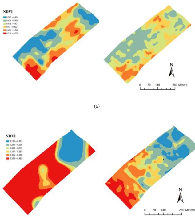
NDVI and yield can now be predicted, by substituting values of on-line measured soil 376
properties into Eq. (8) using coefficients shown in Table 5. A map showing the spatial 377
distribution of predicted versus measured NDVI and yield is shown in Fig. 3 and Fig. 4, 378
respectively. 379
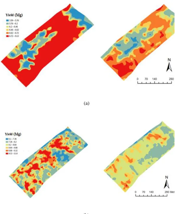
19 381
Observations show that similarities exist between the spatial distributions between each pair 382
of maps, particularly for NDVI. Interestingly, there is a distinct similarity between NDVI and 383
yield maps in 2013 (high r values in Table 6) for both measured and predicted maps (Figs. 3 384
and 4). Conversely, similarities in 2015 for both measured and predicted maps are not clear 385
(low r values in Table 6). The poor similarities shown in the 2015 cropping season may be 386
attributed to deterioration in PLSR prediction accuracy for the on-line collected soil data in 387
2015, since PLSR calibration models were developed on the basis of samples collected in 388
2013. This could also explain the drop in the total contribution of soil properties to yield 389
(SERR = 12.51) and low r (Table 6). Anotherpotential explanationisthat external factors not 390
accounted for in this study (e.g., fungi diseases) have a stronger influence on crop yield in 391
2015 than in 2013. 392
Pearson correlation coefficient values shown in Table 6 demonstrate that the prediction 393
performance for NDVI is more successful than yield in three out of four occasions. This 394
observation is supported by the fact that SERR values for NDVI are consistently higher than 395
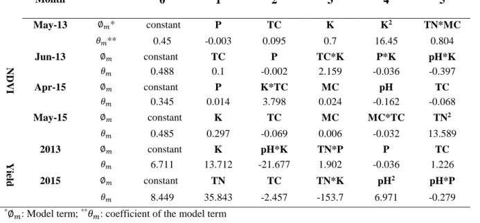
Table 5: Individual and interaction relationship between on-line measured soil properties and normalised difference vegetation index (NDVI) and yield for data collected in 2013 and 2015. The order of the terms was ranked by the calculated individual contribution (ERRC) of each soil property.
Month 0 1 2 3 4 5 NDVI May-13 ∅𝑚* constant P TC K K2 TN*MC 𝜃𝑚** 0.45 -0.003 0.095 0.7 16.45 0.804 Jun-13 ∅𝑚 constant TC P TC*K P*K pH*K 𝜃𝑚 0.488 0.1 -0.002 2.159 -0.036 -0.397 Apr-15 ∅𝑚 constant P K*TC MC pH TC 𝜃𝑚 0.345 0.014 3.798 0.024 -0.162 -0.068 May-15 ∅𝑚 constant K TC MC MC*TC TN2 𝜃𝑚 0.485 0.297 -0.069 0.006 -0.032 13.589 Yield 2013 ∅𝑚 constant K pH*K TN*P P TC 𝜃𝑚 6.711 13.712 -21.677 1.902 -0.036 1.226 2015 ∅𝑚 constant TN TC TN*K pH2 pH*P 𝜃𝑚 8.449 35.843 -2.457 -153.7 6.971 -0.279 *∅
20
the corresponding values for yield (Tables 3 and 4). The highest SERR value of 48.59% is 396
calculated for NDVI prediction in April 2015 (Table 4), which is in line with the highest r 397
value of 0.71 calculated between measured and predicted values (Table 6). 398
399
Although r values are larger for NDVI than for yield during the two cropping seasons (Table 400
6), it is not recommended to rely on only the six on-line measured soil properties to predict 401
yield. Low r values for yield could be attributed to the exclusion of other factors affecting 402
yield and encountered at late growing stages such as soil compaction, inter plant competition, 403
fungal disease and insect pressures (Donald, 1963; Cannell et al., 1980; Coakley, 1988; 404
Paveley et al., 2012). The latter factors have high spatial variability and can reduce yields by 405
up to 7 tonne ha-1 (Bravo et al., 2003). Therefore, it is suggested to expand the current work 406
by accounting for other soil properties and diseases, alongside weather conditions, which is 407
considered the most influential factor controlling the distribution and severity of fungal 408
infections (Dammer, 2006). 409
Table 6: Pearson correlation coefficient (r) values between measured and predicted crop yield and normalised difference vegetation index (NDVI), based on Eq. (8) and identified terms and coefficients shown in Table 5. The crops were wheat and spring barley in 2013 and 2015, respectively.
Year Output Correlation coefficient
2013 Yield 0.48 2015 Yield 0.38 2013 NDVI May 0.56 2013 NDVI June 0.60 2015 NDVI April 0.71 2015 NDVI May 0.40
2013 NDVIm (May) vs Yieldm 0.60
2013 NDVIp (May) vs Yieldm 0.40
2013 NDVIp (May) vs Yieldp 0.83
2015 NDVIm (April) vs Yieldm 0.12
2015 NDVIp (April) vs Yieldm 0.10
2015 NDVIp (April) vs Yieldp 0.25
The significance threshold is 0.062 at 95% confidence level, NDVIm is measured NDVI, NDVIp is predicted NDVI, Yieldm is measured yield and Yieldp is predicted yield
21 410
This study has presented a novel application of nonlinear parametric modelling technique 411
based on a Volterra Nonlinear Regressive with eXogenous inputs (VNRX) model to study the 412
influences of six soil properties: total nitrogen (TN), total carbon (TC), moisture content 413
(MC), potassium (K), phosphorous (P) and pH. Soil properties were collected at high 414
(a)
(b)
Fig. 3. Comparison between measured (right) and predicted (left) normalised difference vegetation index (NDVI) based on Eq. (8) and corresponding terms and coefficients shown in Table 5 for May 2013 (a) and April 2015 (b).
22
sampling resolution with an on-line soil sensor on crop yield and normalised difference 415
vegetation Index (NDVI). The analysis was carried out in two cropping seasons in 2013 416
(wheat) and 2015 (spring barley). The results provided for the following conclusions: 417
(a)
(b)
Fig. 4. Comparison between measured (right) and predicted (left) crop yield using the model of Eq. (8) and corresponding terms and coefficients shown in Table 5 for wheat in 2013 (a), and spring barley in 2015 (b).
23
1. The performance of the VNRX model in the prediction of yield evaluated with the 418
error reduction ratio contribution (ERRC) indicated that different soil properties have 419
different influences on yield. K, P and TC were the highest contributors to wheat yield 420
and TN, TC and P to spring barley. 421
2. Sum of error reduction ratio (SERR) showed soil property contributions to NDVI to 422
be higher than those to yield, with TC, K and P being the most influencing factors. 423
The highest SERR value of 48.59% was calculated for NDVI, which was in line with 424
the highest Pearson correlation coefficient (r) of 0.71 calculated between measured 425
and predicted NDVI. 426
3. The highest influential interaction terms of soil properties on NDVI were TC * K, and 427
MC * TC, whereas the most important terms for yield were pH * K and TN * P for 428
wheat and TC * K and pH * P for spring barley. These contributions may vary among 429
different fields, crops, weather conditions and soil fertility status. 430
4. Although VNRX models allowed the prediction of yield and NDVI to a given degree 431
of success, relatively low correlations between measured and predicted yield 432
necessitate a need to understand other influencing factors (i.e., weather conditions, 433
disease and other soil properties), to improve VNRX model predictions. 434
Acknowledgements 435
We acknowledge the funding received for FarmFUSE project from the ICT-AGRI under the 436
European Commission’s ERA-NET scheme under the 7th Framework Programme, and the 437
UK Department of Environment, Food and Rural Affairs (contract no: IF0208). 438
References 439
Adamchuk, V.I., Morgan, M.T., and Ess, D.R., 1999. An automated sampling system for measuring 440
soil pH. Transactions of the ASABE. 42(4), 885-891. 441
24
Ashraf, M.Y., 1998. Photosynthetic efficiency of wheat under water stress conditions. Journal of
442
Scientific & Industrial Research. 41, 151-163. 443
Baligar, V.C., Fageria, N.K. and He, Z.L., 2001. Nutrient use efficiency in plants. Communications in
444
Soil Science and Plant Analysis. 32(7-8), 921-950. 445
Bigg, G. R., Wei, H. L., Wilton, D. J., Zhao, Y., Billings, S. A., Hanna, E., and Kadirkamanathan, V., 446
2014. A century of variation in the dependence of Greenland iceberg calving on ice sheet 447
surface mass balance and regional climate change. Proceedings of the Royal Society A:
448
Mathematical, Physical and Engineering Sciences. 470(2166), 20130662. 449
Billings, S.A., Chen, S. and Korenberg, M.J., 1989. Identification of MIMO nonlinear systems using a 450
forward regression orthogonal estimator. International Journal of Control. 49, 2157–2189. 451
Boone, L., Van linden, V., De Meester, S., Vandecasteele, B., Muylle, H., Roldán-Ruiz, I., Nemecek, 452
T. and Dewulf, J., 2016. Environmental life cycle assessment of grain maize production: An 453
analysis of factors causing variability. Science of The Total Environment. 553, 551-564. 454
Bravo, C., Moshou, D., West, J., McCartney, A. and Ramon, H., 2003. Early disease detection in 455
wheat fields using spectral reflectance. Biosystems Engineering. 84(2), 137-145. 456
British Standard Institute, (BSI), 1995. Determination of organic and total carbon after dry 457
combustion (elementary), BSI 389. Chiswick High Road, London W4 4AL, UK.. 458
British Standard Institute, (BSI), 1998. Determination of particle size distribution in mineral soil 459
material–method by sieving and sedimentation, BSI 389. Chiswick High Road, London W4 460
4AL, UK. 461
British Standards Institute, (BSI), 2007. Sample preparation for chemical and physical tests, 462
determination of dry. UK: British Standards Institute. 463
Cannell, R.Q., Belford, R.K., Gales, K., Dennis, C.W. and Prew, R.D., 1980. Effects of waterlogging 464
at different stages of development on the growth and yield of winter wheat. Journal of the
465
Science of Food and Agriculture. 31(2), 117-132. 466
Cantelmo, C. and Piroddi, L., 2010. Adaptive model selection for polynomial NARX models. IET
467
Control Theory & Applications. 4(12), 2693-2706. 468
Chen, S. and Billings, S.A., 1989. Representation of non-linear systems: the NARMAX model. 469
International Journal of Control. 49, 1013-1032. 470
Christy, C.D., 2008. Real-time measurement of soil attributes using on-the-go near infrared 471
reflectance spectroscopy. Computers and Electronics in Agriculture. 61, 10-19. 472
Coakley, S.M., 1988. Variation in climate and prediction of risk in balanced fertility, control of weeds, 473
field scouting, re-plants. Annual Review of Phytopathology. 26, 163–181. 474
25
Dammer, K.H. and Ehlert, D., 2006. Variable-rate fungicide spraying in cereals using a plant cover 475
sensor. Precision Agriculture. 7(2), 137-148. 476
Donald, C.M., 1963. Competition among crop and pasture plants. Academic Press. 477
Eberhart, S.T. and Russell, W. A., 1966. Stability parameters for comparing varieties. Crop science.
478
6(1), 36-40. 479
Frogbrook, Z.L and Oliver, M.A., 2007. Identifying management zones in agricultural fields using 480
spatially constrained classification of soil and ancillary data. Soil Use and Management. 23(1), 481
40-51. 482
Grant, C.A., Flaten, D.N., Tomasiewicz, D.J. and Sheppard, S.C., 2001. The importance of early 483
season phosphorus nutrition.Canadian Journal of Plant Science.81(2),211-224. 484
Khosla, R., Inman, D., Westfall, D. G., Reich, R. M., Frasier, M., Mzuku, M., Koch, B. and Hornung, 485
A., 2008. A synthesis of multi-disciplinary research in precision agriculture: site-specific 486
management zones in the semi-arid Western Great Plains of the USA. Precision Agriculture.
487
9, 85-100. 488
Mitscherlich, E.A., 1909. The law of the minimum and the law of diminishing soil productivity. 489
Landwirtschqfliche Jahrbuecher. 38, 537–552. 490
Mouazen, A. M., Maleki, M.R., De Baerdemaeker, J. and Ramon, H., 2007. On-line measurement of 491
some selected soil properties using a VIS-NIR sensor. Soil & Tillage Research. 93, 13–27. 492
Mouazen, A. M., Alhwaimel, S. A., Kuang, B. and Waine, T., 2014. Multiple on-line soil sensors and 493
data fusion approach for delineation of water holding capacity zones for site specific 494
irrigation. Soil & Tillage Research. 143, 95-105. 495
Mouazen, A., De Baerdemaeker, J. and Ramon, H., 2006. Effect of wavelength range on the 496
measurement accuracy of some selected soil constituents using visual-near infrared 497
spectroscopy. Journal of Near Infrared Spectroscopy. 14, 189–199. 498
Mouazen, A.M., 2006. Soil survey device. BE Patent WO/2006/015463. 499
Mouazen, A.M., De Baerdemaeker, J. and Ramon, H., 2005. Towards development of on-line soil 500
moisture content sensor using a fibre-type NIR spectrophotometer. Soil & Tillage Research.
501
80(1-2), 171-183. 502
Murphy, J. and Riley, J. P., 1962. A modified single solution method for determination of phosphate 503
in natural waters. Analytica Chimica Acta. 27, 31–36. 504
Nicholls, C. Soils 5: pH and Nutrients. HGCA. 26 11 2015. 505
http://www.fwi.co.uk/academy/lesson/soils-5-ph-and-nutrients (accessed 04 22, 2016). 506
26
Olsen, S. R., Cole, C.V., Watanabe, F.C. and Dean, L.S., 1954. Estimation of available phosphorus in 507
soil by extraction with sodium bicarbonate. Circular / United States Department of 508
Agriculture, 939. 509
Ozanne, P. G.,1980. Phosphate nutrition of plants -A general treatise. In: Khasawneh, F.E., Sample, 510
E. C. and Kamprath, E. J. Editors. The Role of Phosphorus in Agriculture. American Society 511
of Agronomy. Madison,pp.559-589. 512
Paveley, N., Blake, J., Gladders, P. and Cockerell, V., 2012. Wheat disease management guide.
513
HGCA. 514
Ravikumar, P., 2013. Evaluation of nutrient index using organic carbon, available P and available K 515
concentrations as a measure of soil fertility in Varahi River basin, India. Proceedings of the
516
International Academy of Ecology and Environmental Sciences. 330. 517
Renouf, M.A., Wegener, M.K. and Pagan, R.J., 2010. Life cycle assessment of Australian sugarcane 518
production with a focus on sugarcane growing. The International Journal of Life Cycle
519
Assessment. 15(9), 927–937. 520
Roy, R.N., Finck, A., Blair, G.J. and Tandon, H.L.S, 2006. Plant nutrition for food security. Rome, 521
Italy: Food and Agriculture Organization of the United Nations. 522
Sarrigiannis, P.G., Zhao, Y. Wei, H.L., Billings, S.A., Fotheringham, J. and Hadjivassiliou, M., 2014. 523
Quantitative EEG analysis using error reduction ratio-causality test; validation on simulated 524
and real EEG data. Clinical Neurophysiology. 125(1), 32–46. 525
Schubert, S., Schubert, E. and Mengel, K., 1990. Effect of low pH of the root medium on proton 526
release, growth, and nutrient uptake of field beans (Vicia faba). Plant and Soil. 124(2), 239-527
244. 528
Shaddad, S., 2013. Proximal soil sensors and geostatistical tools in precision agriculture applications.
529
Sassari, Italy: Universita Degli Studi Di Sassari. 530
Shaddad, S.M., Madrau, S., Castrignanò, A. and Mouazen, A.M., 2016. Data fusion techniques for 531
delineation of site-specific management zones in a field in UK. Precision Agriculture. 17(2), 532
200-217. 533
Shibusawa, S., Imade Anom, S.W., Sato, A., Sasao, A. and Hirako, S, 2011. Soil mapping using the
534
real-time soil spectrophotometer. Vol. 1, in Third European Conference on Precision
535
Agriculture, by G. Grenier and S. Blackmore, pp. 497–508. Montpellier, France: ECPA. 536
Soil Survey Staff, 1999. Soil Taxonomy - A basic system of soil classification for making and 537
interpreting soil surveys; second edition. Agricultural Handbook 436; Natural Resources 538
Conservation Service, USDA. Washington DC, USA.
27
Tashev, I.J., 2009. Sound Capture and Processing: Practical Approaches. John Wiley & Sons. 540
Viscarra Rossel, R.A., Walvoort, D.J.J., McBratney, A.B., Janik, L.J. and Skjemstad, J.O., 2006 541
Visible, near infrared, mid infrared or combined diff use. Geoderma. 131, 59–75. 542
Wei, H.L., Billings, S.A. and Liu, J., 2004. Term and variable selection for nonlinear system 543
identification. International Journal of Control. 77, 86-110. 544
Zadoks, J.C., Chang, T.T. and Konzak, C.F.,1974.A decimal code for the growth stages of cereals. 545
Weed Research.14(6),415–421. 546
Zhao, Y., Bigg, G.R., Billings, S.A., Hanna, E., Sole, A.J., Wei, H., Kadirkamanathan, K. and Wilton, 547
D.J., 2016. Inferring the variation of climatic and glaciological contributions to West 548
Greenland iceberg discharge in the twentieth century. Cold Regions Science and Technology.
549
121, 167–178. 550
Zhao, Y., Wei, H.L. and Billings, S.A., 2012. A New Adaptive Fast Cellular Automaton 551
Neighborhood Detection and Rule Identification Algorithm. IEEE Transactions on Systems,
552
Man, and Cybernetics—Part B: Cybernetics. 42(4), 1283-1287. 553
Zhao, Y., Mehnen, J., Sirikham, A. and Roy, R., 2017. A novel defect depth measurement method 554
based on Nonlinear System Identification for pulsed thermographic inspection. Mechanical
555
Systems and Signal Processing. 85, 382–395. 556
Zhao, Y., Billings, S.A., Wei, H. and Sarrigiannis, P.G., 2012. Tracking time-varying causality and 557
directionality of information flow using an error reduction ratio test with applications to 558
electroencephalography data. Physical Review E. 86, 051919. 559