LBS Research Online
N Hirschey
Do high-frequency traders anticipate buying and selling pressure? Article
This version is available in the LBS Research Online repository: http://lbsresearch.london.edu/
1458/ Hirschey, N
(2020)
Do high-frequency traders anticipate buying and selling pressure?
Management Science. ISSN 0025-1909 (In Press)
DOI:https://doi.org/10.1287/mnsc.2020.3608
INFORMS (Institute for Operations Research and Management Sciences)
https://pubsonline.informs.org/doi/10.1287/mnsc.20...
Users may download and/or print one copy of any article(s) in LBS Research Online for purposes of research and/or private study. Further distribution of the material, or use for any commercial gain, is not permitted.
Do High-Frequency Traders Anticipate Buying and
Selling Pressure?
Nicholas Hirschey * London Business School
January 2020
Abstract: This study provides evidence that high-frequency traders (HFTs) identify patterns in past trades and orders that allow them to anticipate and trade ahead of other investors’ order flow. Specifically, HFTs’ aggressive purchases and sales lead those of other investors, and this effect is stronger at times when it is more difficult for non-HFTs to disguise their order flow. Consistent with some HFTs being more skilled or more focused on anticipatory strategies, I show that trades from a subset of HFTs consistently predict non-HFT order flow the best. The results are not explained by HFTs reacting faster to news or past returns, by contrarian or trend-chasing behavior by non-HFTs, or by trader misclassification. These findings support the existence of an anticipatory trading channel through which HFTs increase non-HFT trading costs.
*Contact information: Department of Finance, London Business School, Regent’s Park, London NW1 4SA, United
Kingdom; Email: nhirschey@london.edu. I would like to thank NASDAQ OMX for providing the data and Frank Hatheway, Claude Courbois, and Jeff Smith for many useful discussions about the data and market structure. I would also like to thank Andres Almazan, Fernando Anjos, Robert Battalio, Johannes Breckenfelder, Carlos Carvalho, Jonathan Cohn, Shane Corwin, Andres Donangelo, Cesare Fracassi, John Griffin, Terry Hendershott, Paul Irvine, Pete Kyle, Richard Lowery, Tim Loughran, Jeffrey Pontiff, Mark Seasholes, Clemens Sialm, Laura Starks, Sheridan Titman, and seminar participants at Boston College, the European Finance Association meeting, the Georgia Institute of Technology, the Hong Kong University of Science and Technology, the London Business School, the London School of Economics, Rice University, the University at Buffalo, the University of California Irvine, the University of Georgia, Manchester Business School, the University of Melbourne, the University of Miami, the University of Notre Dame, the University of Texas at Austin, and the Western Finance Association meeting for helpful comments and suggestions.
Investors and regulators have immense interest in the automated strategies used by high-frequency traders (HFTs) and how they affect other investors. Liquidity provision by HFTs has clear benefits. Yet HFTs make many informed trades; more than half their dollar volume on NASDAQ comes from marketable trades that must predict returns to be profitable. The welfare consequences of this informed trading are less clear. In particular, a prominent concern is that one way HFTs predict returns is by using past trade and order data to learn which stocks non-HFTs are about to buy or sell. This information is valuable because an HFT who infers a non-HFT is beginning to liquidate a large position can sell shares now and profit when the price subsequently falls.
This paper examines these issues and provides the first evidence that one reason HFTs appear informed is that they anticipate and trade ahead of non-HFT buying and selling pressure. Specifi-cally, I analyze return and trade patterns around periods of intense marketable buying and selling by HFTs. The imbalance between these marketable purchases and sales is a simple measure of HFTs’ directional bets.1 Anticipatory trading implies HFTs trade in the same direction as their expectation of future non-HFT order flow. Consistent with HFTs using such a strategy, I show that when HFTs sell a stock with marketable orders, this predicts future marketable selling by non-HFTs and lower returns.
This strategy has important implications for liquidity and price efficiency. If a non-HFT is selling to fund a liquidity shock, the HFT’s selling harms the non-HFT by depressing their liquidation price (Brunnermeier and Pedersen 2005). If instead the non-HFT is selling because the stock is overvalued, the HFT is effectively reverse engineering the non-HFT’s signal (Madrigal 1996, Yang and Zhu 2019, Baldauf and Mollner 2020). Competition between the HFT and non-HFT to trade on the signal causes prices to incorporate this information faster.2 But it also implies moderated benefits of HFT participation in price discovery, because some information arriving via HFT trades would soon be incorporated into prices by non-HFTs anyway. Additionally, the competition lowers non-HFT profits, which reduces their incentive to acquire information (Grossman and Stiglitz 1980,
1A marketable limit order is functionally equivalent to a market order: a buy order with a limit price at or above
the best ask or a sell order with a limit price at or below the best bid at the time it enters the order book. NASDAQ requires all orders to have a limit price, and a trade is initiated when a marketable limit order crosses either the best bid or best ask.
2Non-HFTs may at first trade less aggressively to hide from HFTs, slowing price adjustment. But once the HFT
has learned how the non-HFT is trading, competition between them ultimately pushes prices closer to fundamental value (Madrigal 1996, Yang and Zhu 2019).
Stiglitz 2014, Weller 2018).3 These concerns were the basis for Michael Lewis’s (2014) book, Flash Boys, and the founding of the deliberately slowed down IEX trading platform.
The analysis in this paper uses an entire year of unique trade and trader-level data from the NASDAQ Stock Market. It is an important sample for studying HFTs given NASDAQ was the biggest U.S. exchange by volume and HFTs accounted for 40% of its dollar volume.
In tests where stocks are sorted by HFT net marketable buying at the one second horizon, non-HFT net marketable buying for the stocks bought most aggressively by non-HFTs rises by a cumulative 65% of its one-second standard deviation over the following thirty seconds. For the median stock, this equates to a 100 share HFT imbalance predicting non-HFTs to buy 13 more shares with marketable orders than they sell. The figures for stocks HFTs sell most aggressively are similar, but in the opposite direction. Turning to returns, future returns for stocks HFTs buy aggressively are positive, while returns for stocks they sell aggressively are negative. The returns and non-HFT trade imbalances predicted by these sorts persist for more than five minutes.
The sorts also show who provides liquidity to these marketable HFT trades. For the stocks HFTs buy with marketable trades, their net buying is also positive in the surrounding seconds. Thus at these times HFTs in aggregate take liquidity from non-HFTs.
The evidence is consistent with HFTs recognizing persistent informed non-HFT order flow in real time. Since liquidity providers are slow to update their quotes, HFTs trade ahead of the impending non-HFT order flow and associated price change to earn a profit. I provide two example patterns that illustrate how HFTs could identify stocks with persistent order flow and prices that update slowly. The examples are simple, interpretable, and use only past order flow and returns as their inputs. Though HFTs use more sophisticated algorithms, the example patterns nonetheless succeed in predicting future non-HFT order flow and returns. And HFT order flow in surrounding seconds is consistent with the patterns capturing predictability used by HFTs.
I next examine whether some HFTs are more skilled at anticipating order flow. There is evidence HFTs follow a variety of strategies (Boehmer, Li, and Saar 2018) and fast HFTs are more profitable (Baron, Brogaard, Hagstr¨omer, and Kirilenko 2019). Consistent with HFTs having heterogenous skills, there is persistence in which individual HFTs’ trades most strongly predict non-HFT order
3These incentive effects arise when HFTs learn from the endogenous order flow of non-HFTs who pay a cost for
their signals. This is absent from models in which the speculative HFT’s trades do not affect the signal itself, such as Foucault, Hombert, and Rosu (2016).
flow. I sort HFTs into three groups each month based on the size of coefficients from regressions of non-HFT order flow on the HFTs’ lagged trading (excluding predictability from trend-chasing by non-HFTs and serial correlation in non-HFT order flow). For HFTs in the top third the prior month, a one-standard deviation shock to their net marketable buying predicts a cumulative change in non-HFT net marketable buying equal to 14% of its one-second standard deviation over the next 30 seconds. This compares to an estimate of 2% for HFTs in the bottom third. These top HFTs’ trades are also more strongly correlated with future returns. This skill persistence result holds regardless whether individual HFTs are sorted based on correlations with their net marketable buying or total net buying (summing marketable and non-marketable trades).
These findings imply that large non-HFTs have an incentive to disguise their order flow, and in reality we see them deploy execution algorithms to achieve this goal. Yet in the competition between HFT and non-HFT algorithms, non-HFTs are at a disadvantage to the extent that they are constrained by their desire to enter or exit their position. Dark pool operator ITG writes, “some traders are more willing to increase fill rate at the expense of execution quality—the risk of information leakage and impact”(ITG 2013). Indeed, I find the correlation between HFT and non-HFT trades is stronger at times non-non-HFTs are impatient and thus less focused on disguising order flow: at the market open, on days with high volume, and when trading illiquid or small-cap stocks. This is consistent with Goldman Sachs’ acknowledgement their algorithms leak more information in small-caps (Traders Magazine 2013).
I consider several explanations for marketable HFT trades leading marketable non-HFT trades. The effect could be caused by HFTs reacting faster to a signal non-HFTs also observe (Von Beschwitz, Keim, and Massa 2015, Chordia, Green, and Kottimukkalur 2018). But the most probable signals they would both utilize in close succession do not fully explain the results (e.g., past returns, news articles, analyst forecasts and recommendations, management guidance, and form 8-K filings). Con-trols for returns also show the effect is not due to a reverse causality story in which HFT purchases cause trend chasing non-HFTs to purchase shares as well. Another explanation is trade misclassi-fication. Perhaps NASDAQ incorrectly labels some HFT trades as coming from non-HFTs. Then the lead-lag result may be caused by trades from correctly labeled HFTs predicting those of incor-rectly labled HFTs who follow similar strategies. I evaluate this explanation by comparing the way HFT trading forecasts itself to how it forecasts non-HFT trading. Misclassification implies that
non-HFT predictability comes from it being a noisy proxy for HFT trading, so HFT trading should predict itself better than non-HFT trades. Once you look more than seven seconds into the future, HFT marketable trades forecast non-HFT marketable trades more strongly than HFT marketable trades. By 15 seconds later, HFT marketable trading no longer forecasts itself, whereas it continues to forecast non-HFT marketable trading for more than 30 seconds.
Another question is whether the results are more consistent with HFTs trading ahead of order flow to avoid losses on market making inventory positions or to profit from speculation. To evaluate this question, I examine cumulative HFT net buying for stocks in extreme HFT net marketable buying portfolios before and after the sort second. There is no evidence marketable HFT trades are predominately caused by inventory management. It is possible the marketable trades are disposing of inventory acquired on exchanges other than NASDAQ. However, additional evidence is more consistent with a speculative interpretation. Marketable trades are more than half of HFT volume, which is inconsistent with a pure risk management motive. Additionally, HFT trades lead non-HFT trades more strongly early in the trading day and in small-cap stocks, whereas inventory risk is more binding towards the end of the day and HFT market making is more prevalent in large-cap stocks (Yao and Ye 2018).
This paper makes an important contribution to our understanding of predictability in order flow. In a lower frequency context, Barbon, Di Maggio, Franzoni, and Landier (2019) and Di Maggio, Franzoni, Kermani, and Sommavilla (2019) show evidence of non-HFT brokers leaking information about one non-HFT client’s trades to other non-HFT clients. Clark-Joseph (2013) studies a form of anticipatory trading in S&P 500 futures, though his focus is whether HFTs use small trades to learn about price impact. Recent work using data from Canada (Korajczyk and Murphy 2019) and Sweden (Van Kervel and Menkveld 2019) shows HFTs initially providing liquidity at the start of large multi-hour institutional orders before switching to trade in the same direction as the institutional order after 30 or more minutes.4 Using U.S. equities data, this paper complements those studies by showing that if you condition on higher frequency second-by-second data, you observe HFTs taking liquidity ahead of non-HFTs at more favorable prices. I also provide evidence that HFTs’ ability to predict order flow is not limited to the latter part of large orders. Specifically,
4Reiss and Werner’s (1998) evidence on dealers trading ahead of worked orders is also related, though in their
HFT marketable trades predict non-HFT marketable trades more strongly the first half hour of trading, which is necessarily early in a multi-hour order. And the second-level spikes in HFT marketable imbalances coincide with spikes in non-HFT marketable imbalances, which shows the patterns in this paper are distinct from longer-term trends.
These findings relate to a broader debate about the merits of modern market structure.5 Re-search shows that faster trading technology and more HFT liquidity provision are generally asso-ciated with improvements in common liquidity measures.6 There is also evidence a fair portion of price discovery comes from algorithmic traders in general (O’Hara, Yao, and Ye 2014) and HFTs in particular (Brogaard, Hendershott, and Riordan 2014, 2019). But while the net effect of the transition to electronic markets may be positive, there are also channels through which fast trading can have a negative impact. Examples include increased liquidity provider losses to cross-market arbitrage (Budish, Cramton, and Shim 2015) and to news trading (Menkveld and Zoican 2017).
This paper highlights another negative channel. It shows one way HFTs predict returns is by extracting information from informed non-HFT order flow. This is important, because a non-HFT whose trades are anticipated either trades fewer shares than they desire or obtains executions at a worse average price. These effects are hard to detect with standard liquidity measures. Doing so requires conditioning on the magnitude of a non-HFT’s liquidity shock or, if the non-HFT is informed, the magnitude of their signal. I use a structural VAR to provide a rough estimate. The results imply non-HFT price impact is 14% higher when they compete with HFTs using anticipatory strategies.
1
Hypothesis Development
A speculator able to predict marketable trade imbalances could use this information to predict returns and earn a profit (e.g., Madrigal (1996), Brunnermeier and Pedersen (2005), and Yang and
5Other issues include the effects of alternative trading venues (Foucault and Menkveld 2008, O’Hara and Ye
2011, Comerton-Forde and Putnin,ˇs 2015), tick size (Chao, Yao, and Ye 2016, Yao and Ye 2018, O’Hara, Saar, and Zhong 2019), high-frequency volatility (Kirilenko, Kyle, Samadi, and Tuzun 2017, Hasbrouck 2018, Egginton, Van Ness, and Van Ness 2016), overinvestment in technology (Biais, Foucault, and Moinas 2015), and agency conflicts caused by exchange fee rebates (Battalio, Corwin, and Jennings 2016).
6Examples include Hendershott, Jones, and Menkveld (2011), Boehmer, Fong, and Wu (2015), Hendershott and
Riordan (2013), Hasbrouck and Saar (2013), Conrad, Wahal, and Xiang (2015), Conrad and Wahal (2019), Brogaard, Hagstromer, Norden, and Riordan (2016), Jovanovic and Menkveld (2015), Menkveld (2013), Breckenfelder (2013), Brogaard and Garriott (2019), Ait-Sahalia and Saglam (2016), Brogaard, Carrion, Moyaert, Riordan, Shkilko, and Sokolov (2017), and Griffith, Van Ness, and Van Ness (2017).
Zhu (2019)). The idea is supported by evidence that marketable purchases lead to price increases and marketable sales lead to price declines (Hasbrouck 1991). This happens because trades may contain information about fundamental values (Glosten and Milgrom 1985, Kyle 1985) or cause liquidity providers to take risky positions (Stoll 1978).
HFTs are good candidates for speculators who learn about order flow. Doing so requires fast trading technology and automated analysis of quote updates and trades. And HFTs specifically invest in these technologies.
This anticipatory trading hypothesis can be tested by comparing the timing of HFT marketable trades to non-HFT marketable trades. Assume an HFT identifies a signal indicating there will be non-HFT marketable selling in the near future. If the liquidity provider has not conditioned on this signal, then the liquidity provider’s bid will be too high. The HFT should sell the stock with a marketable limit order that hits the bid. Afterwards, non-HFTs will similarly sell with marketable orders, driving the price lower and creating a profit for the HFT.
Hypothesis 1 HFT net marketable buying will be positively correlated with future non-HFT net marketable buying and returns.
In principle, the HFT could also sell with a non-marketable order, but much of the variation in HFTs’ non-marketable orders is caused by liquidity provision. By focusing on HFTs’ marketable orders, I instead focus on times when their trades are more likely to be caused by information.
The second main hypothesis seeks to determine whether HFTs are anticipating non-HFTs trad-ing for information or liquidity reasons. Price changes after HFTs’ trades provide insight into which of these explanations is more typical.
Hypothesis 2 If HFTs anticipate informed order flow, price changes predicted by their marketable trades will be permanent, whereas if they anticipate uninformed order flow, the price changes will be temporary.
There are many plausible ways HFTs could learn about order flow. The one I emphasize is insufficiently disguised positive serial correlation in order flow. Marketable buying is known to have positive serial correlation (Hasbrouck 1991, Chordia, Roll, and Subrahmanyam 2002). This can arise from splitting a large order into small trades executed over time. Order splitting is
generally optimal for a trader who has discretion over when to trade, and it is useful for both informed traders (Kyle 1985) and liquidity traders (Vayanos 2001). But this practice leaves open the possibility that in executing the first part of an order, a large trader reveals more than he intends. A similar type of information leakage can occur when a trader simultaneously sends orders for a stock to different exchanges (e.g., NYSE and NASDAQ), but routing complications cause the orders to arrive at those venues at different times (Lewis 2014). These signals may be profitable to use if liquidity providers do not condition on them when setting bid-ask quotes.
Hypothesis 3 One way HFTs profit from anticipatory trading is by identifying times when prices have not updated to account for positive serial correlation in non-HFT order flow.
The final main hypothesis relates to understanding differences between HFTs. Anticipatory trading requires an HFT to be more skilled than some liquidity providers at learning from order flow. Additionally, we do not expect different HFTs to follow the same strategies (Boehmer, Li, and Saar 2018). It follows that anticipatory trading may be concentrated in a subset of the HFTs.
Hypothesis 4 If certain HFTs are better at forecasting order flow or focus more on the strategy, then trades from these HFTs will be consistently more strongly correlated with future non-HFT trades than trades from other HFTs.
These hypotheses are not biased by using exclusively NASDAQ data. A finding that HFTs make marketable purchases and sales immediately before non-HFTs on NASDAQ is true regardless of what is happening on other exchanges and regardless of the HFTs’ net position across all exchanges. To reverse this finding across all markets, it would be necessary to find the reverse pattern elsewhere. But there is no reason to believe NASDAQ is not representative. It was the biggest exchange, market structure has convergenced to electronic limit order books everywhere, and mostly the same HFTs and non-HFTs trade on all exchanges.
2
Data
2.1 Sample construction
This study uses intra-day transactions data from the NASDAQ Stock Market. NASDAQ was the largest U.S. exchange by volume during the January to December 2009 sample period,7 with a 21.3% share of total volume (NASDAQ 10K 2009). This includes 33.0% of NASDAQ-listed volume and 15.7% of NYSE-listed volume. Like all exchanges, it is structured as an electronic limit-order book and executions primarily come from professional traders.8
The 96 sample stocks (48 NASDAQ-listed and 48 NYSE-listed) are randomly selected from a sample universe representative of the stocks traded by actively managed investment funds. I use a random sample instead of all common stocks because of computational constraints. The sample is constructed from single-class CRSP common stocks (share code 10 or 11) at the end of 2008. I exclude the bottom two NYSE size deciles to approximate common definitions of active funds’ investable universe (e.g., Russell 3000 or MSCI Investable Market 2500). To ensure sample stocks are fairly liquid, I require greater than $1 million average daily dollar volume in December 2008 and a stock price greater than $5 at the end of 2008. From this sample universe of 1,882 stocks, I then randomly select 6 NASDAQ-listed and 6 NYSE-listed stocks from each of the eight remaining size deciles.
Table 1 reports summary statistics for all stock days in the sample. The sample averages 93 stocks per trading day.9 Market capitalization ranges from $22 million to $125,331 million. On average, 27.2% of the stocks’ dollar volume trades on NASDAQ, and this varies little across size portfolios. Comparing small-caps to mid- and large-caps, as market capitalization increases, there are increases in median price ($14.77, $25.04, and $31.37 ), median dollar volume ($1.9 million, $15.5 million, and $120.2 million), and median HFT share of dollar volume (14.8%, 29.2%, and 40.9%).
7I exclude January 27thfrom the sample, because quote data for NYSE-listed stocks is missing.
8Most retail brokerages have contracts with market making firms who pay for the right to fill retail orders. For
example, in Q3 2009 E*Trade routed nearly all its customers’ market orders and over half its customers’ limit orders to either Citadel or E*Trade’s market making arms (E*Trade 2009). See Battalio and Loughran (2008) for a discussion of these relationships.
9The number of stocks varies for two reasons: first, to ensure tick size does not constrain price movements, stocks
are temporarily removed any day the prior close is less than $1; second, to remove stocks that stop trading due to bankruptcy or acquisition, stocks are permanently removed from the sample after a day with dollar volume less than $100,000. These filters use past rather than future data to avoid look-ahead biases.
2.2 Background on HFTs
The firms typically described as HFTs are trading firms using high-turnover automated strategies. Examples include Tradebot Systems, Inc., and GETCO. These firms are remarkably active traders. On their websites, Tradebot says they often account for more than 5% of total U.S. equity trading volume, and GETCO says they are “among the top 5 participants by volume on many venues” (Tradebot 2010, GETCO 2010). They are a large part of the market. The TABB Group estimated HFTs accounted for 61% of U.S. Equity share volume in 2009 (Tabb 2009).
2.3 HFT identification
The NASDAQ trade data classifies firms as either an HFT or a non-HFT. NASDAQ does not disclose the identities of the HFTs or exact criteria used to determine the classification. This HFT versus non-HFT classification is the same as in Brogaard, Hendershott, and Riordan (2014), though their dataset is different. NASDAQ identifies HFTs using a variety of qualitative and quantitative criteria. The firms classified as HFTs typically use low-latency connections and trade more actively than other investors. Their orders have shorter durations than other investors, and they show a greater tendency to flip between long and short positions in a stock during a day.
A disadvantage of the classification scheme is that it is largely done at the broker level. As a result, HFT orders routed through the standard trading system of a broker that handles non-HFT orders, such as Goldman Sachs or Morgan Stanley, will be misclassified as non-HFT (Brogaard, Hendershott, and Riordan 2014). This is a concern primarily for HFTs that are internal divisions of larger investment banks. Independent HFTs who act as their own broker or who use specialist brokers to co-locate servers and retain direct control of their routing infrastructure should be classified correctly. Section 4.3 evaluates whether potential misclassification has an important effect on the empirical results.
2.4 Construction of returns and trade imbalances
I calculate intra-day returns using cleaned bid-ask midpoints from the National Best Bid and Best Offer (NBBO).10 The NBBO aggregates quotes from all exchanges, so it is the best measure of a
10 The cleaning procedure follows guidelines in Hasbrouck (2010). First, I remove quote updates where the bid
stock’s quoted price.
I use all trades during regular continuous trading hours (no open or closing cross) to con-struct net marketable buying and net buying imbalances. Marketable trades consist of all liquidity-removing sides of transactions. Non-marketable trades include all liquidity-providing sides of trans-actions (both visible and hidden orders). The NASDAQ matching engine makes this marketable/non-marketable designation when a trade is executed. All orders are limit orders, and a trade is initiated when someone submits a limit order that crosses the spread. The matching engine marks the order from the party who initiated the transaction as a marketable order and the other party’s order as non-marketable.
A net marketable buying imbalance, defined as shares in buyer-initiated trades minus shares in seller-initiated trades, is a common measure of buying and selling pressure from the existing literature (e.g., Chordia, Roll, and Subrahmanyam 2002). The net buying imbalance is shares bought minus shares sold and is used to measure position changes of different investor groups. To put trade imbalances on a similar scale across stocks, I normalize all imbalance measures by a stock’s 20-day trailing volume from CRSP.
Panel B in Table 1 summarizes trade imbalances for the sample stocks prior to their being normalized by trailing volume. The table describes the distribution of the stock-day standard de-viations of HFTs’ net buying, their net marketable buying, and non-HFTs’ net marketable buying. The mean standard deviation of HFTs’ net buying (HF TNB) for all stock days is 83 shares,
com-pared to 80 shares for their net marketable buying (HF TN MB). These figures are slightly smaller
than the 100 shares that O’Hara, Yao, and Ye (2014) report as the median trade size on NAS-DAQ in 2008 and 2009. The average standard deviation of non-HFTs’ net marketable buying (non-HF TN MB), at 125 shares, is somewhat higher than that of HFTs. The wide variation in
im-arbitrage that gets corrected within fractions of a second. Second, I remove quotes where the bid-ask spread is more than 20% greater than the bid-ask midpoint. This 20% filter removes rarely occuring stub quotes (e.g., bid at $0.01 and ask at $20.00) that would cause large fluctuations in the bid-ask midpoint that is not reflective of a true price change. The 20% relative spread cutoff for what constitutes reasonable quotes comes from the SEC’s initial single-stock circuit breaker rule. The rule halted stocks after a 10% return in 5 minutes to prevent “clearly erroneous transactions” (SEC 2010). This is consistent with a 20% relative spread limit, because a stock with successive trades first at a negligable spread and then at a 20% relative spread (i.e., bid/ask 10% away from prior trade) would trip the circuit breaker. When an invalid quote is removed due to either filter, I use the last valid midpoint for the price until a new valid midpoint is available. A new midpoint is typically available within a few milliseconds. To remedy bad pre-market quotes in the NYSE data, the last of which is used to proxy for the opening price, I throw out the last price before the open if there is more than a 20% difference between the last pre-open bid-ask midpoint and the first post-open bid-ask midpoint.
balance standard deviations between size portfolios motivates the normalization by trailing volume in later results.
3
Tests of the anticipatory trading hypotheses
This section tests whether HFT trades forecast non-HFT trades and then examines additional empirical implications of the pattern being caused by anticipatory trading.
Throughout the paper, I use a method similar to Fama and MacBeth (1973) to account for cross-sectional correlation across stocks and autocorrelation through time. Observations in nearby seconds are potentially correlated, so they should not be treated as independent. To be conservative, I collapse all estimates on a day to a single average estimate for that day. This gives me a time-series of the average effect each day. I then base hypothesis tests on the mean of that daily time series. In effect, the question I ask is whether the estimate is consistently different from zero throughout the days in the sample. I do not assume observations from the same day are independent. I only assume different days are independent. Of course, there is likely some residual correlation between nearby days, so I use Newey and West t-statistics with the optimal lag length for the daily series chosen following Newey and West (1994). Despite the conservative approach to standard errors, many of the tests show hight-statistics. This happens when the estimated effect is consistent across the days in the sample.
3.1 Do trades from HFTs lead trades from non-HFTs?
Anticipatory trading implies an increase in HFT net marketable buying should forecast an increase in non-HFT net marketable buying and an increase in returns (Hypothesis 1). The first tests use portfolio sorts to examine the hypothesized relationships in a simple and easy to interpret form. Afterward, vector autoregressions (VARs) evaluate whether HFT trading has any predictive power beyond that of past returns and serial correlation in non-HFT trading.
The sorts identify stocks with large HFT net marketable buying imbalances in a given second. I then look at non-HFT net marketable buying and returns afterward.
Every stock is assigned to one of ten portfolios each second based on the stock’s HFT net marketable buying imbalance. Portfolio breakpoints are calculated from non-zero observations
during the prior trading day. Then, a daily mean of the variable of interest for each portfolio is calculated by taking an average among all stock-second observations for the portfolio that day:
Vd,p= 1 Np
X
i,t
Vd,p,i,t,
whereV is the variable of interest,d indexes days,p indexes portfolios, Npis the number of
stock-second observations in the portfolio that day, i indexes stocks, andt indexes seconds. Hypothesis tests are based on the means of these daily time series.
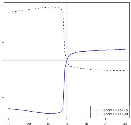
Figure 1 plots cumulative net marketable buying for sort deciles ten (stocks HFTs bought) and one (stocks HFTs sold). Because the figure plots cumulative values, positive net marketable buying causes the line in that second to rise, while negative net marketable buying causes the line to fall. The dark red lines indicate HFTs’ cumulative net marketable buying plotted on the left y-axis. Looking at the stocks HFTs buy, HFT net marketable buying is slightly positive before the sort, spikes in the sort period, and then is relatively flat afterwards. The sort-period spike is expected, because the line is the cumulative value of the variable used to form the portfolios. The real question is what happens to non-HFT net marketable buying afterward.
Consistent with Hypothesis 1, Figure1 shows that in the seconds after these sorts on HFT net marketable buying, non-HFT net marketable buying is positive for the stocks HFTs bought and negative for the stocks HFTs sold. Cumulative non-HFT net marketable buying is depicted by dashed blue lines plotted on the right y-axis. In the seconds after the sort, cumulative non-HFT net marketable buying for the stocks HFTs bought steadily increases. This indicates consistently more marketable purchases than sales—non-HFTs buy the stocks HFTs previously bought. HFTs also buy shares after the sort, but in comparison to non-HFTs, they buy relatively more in the sort second than afterward.
Table 2 presents this sort data in a form conducive to hypothesis tests. Panel A shows that in the first thirty seconds after the sort, cumulative non-HFT net marketable buying rises to 0.65 times the one-second standard deviation (or 27 shares for the median stock). Over the next four and a half minutes, it continues rising to 1.15 (or 48 shares for the median stock). These values are both significantly different from zero, with t-statistics of 14.35 and 2.41. The picture for the stocks HFTs sold most aggressively is symmetric; non-HFT net marketable buying in decile one is
−0.69 and −1.89 times the one-second standard deviation in the first 30 seconds and the first five minutes after the sort respectively.
If the order flow patterns in Figure 1 and Table 2 are due to HFTs anticipating non-HFT buying and selling, then we should also see that the stocks HFTs bought aggressively have positive future returns and the stocks they sold have negative future returns. Figure2shows that in the 30 seconds after the sort, prices of stocks in HFT net marketable buying decile ten increase by 1.23 basis points, while the prices of decile one stocks decline by −1.07 basis points. Table 2B shows both portfolios’ returns are significantly different from zero, with t-statistics of 11.78 and−13.48. These price changes will be permanent if HFTs anticipate order flow from informed traders and temporary if they anticipate liquidity traders (Hypothesis 2). The last two columns in Table 2B show partial reversal of these returns over the next four and a half minutes. Decile ten reverses from 1.23 basis points 30 seconds after the sort to 0.57 basis points five minutes afterwards; decile one reverses from −1.07 to −0.58 basis points. Nonetheless, the return spread between these two portfolios remains positive. This is consistent with Brogaard, Hendershott, and Riordan’s (2014) findings, using a state-space model, that HFT marketable trades forecast permanent price changes. Thus, the evidence is more consistent with HFTs anticipating informed rather than uninformed order flow.
Figure 3 examines who provides liquidity to these marketable HFT trades. In Panel A, stocks are sorted into deciles by HFT net marketable buying the same as in Figure1. The only difference is that I now plot cumulative HFT net buying, which aggregates both marketable and non-marketable trades. A comparison of net marketable buying to net buying reveals who provides liquidity. For example, if one HFT uses a marketable order to purchase 100 shares from another HFT, then net marketable buying across the two HFTs is 100 shares. But net buying is 0, because the first HFT’s purchase and the second’s sale cancel each other out.
Panel A shows that HFTs in aggregate take liquidity from non-HFTs in these sorts. In the sort second, net buying for decile ten rises by 5.77, while it falls by 5.83 for decile one. Averaging the two and multiplying by its median one-second standard deviation (28 shares) gives an average 162 share net position change for either decile. The equivalent calculation for HFTs’ net marketable buying in Figure1 gives a 213 share net marketable imbalance ¡8.19+8.21
2 ×26
¢
. Therefore, 24% of the net liquidity provision comes from HFTs ¡213−162
213 ¢
HFTs’ 37% share of liquidity provision by dollar volume in the sample. The evidence is consistent with HFT liquidity providers stepping away, leaving less-skilled non-HFT liquidity providers to fill informed HFT orders. Panel B explores differences between HFTs, which I defer until Section 3.4. The sorts provide a few additional insights. First, the order flow and return results are stronger in small-cap stocks. In the first 30 seconds after the sort, the difference between non-HFT net marketable buying for the stocks HFTs bought (decile ten) versus sold (decile one) is 2.66 for small-cap stocks, compared to 1.34 for all stocks. Similarly, the decile ten minus decile one return spread is 5.18 basis points for small-cap stocks, compared to 2.30 for all stocks. Both effects persist through five minutes after the sort. The larger post-sort spread in smaller stocks could be due to non-HFTs having a harder time disguising order flow when trading relatively illiquid stocks. Section 3.5 examines this illiquidity hypothesis in more detail. Second, stocks HFTs buy with marketable orders have higher returns the prior 30 seconds (4.43 basis points) than the stocks they sell (−4.30 basis points). The trend chasing is notable, because HFTs are often characterized as liquidity providers. But this pattern is more consistent with these trades demanding liquidity than providing it. Third, that HFT trades predict non-HFT trades at horizons much longer than a second shows the result is not an artifact of cross-market arbitrage. This type of arbitrage is understood to occur at sub-second horizons (see Budish, Cramton, and Shim 2015).
Table 3 builds on the sort results using a vector autoregression (VAR) similar to Hasbrouck (1991). The portfolio sorts show evidence of positive serial correlation and trend-chasing in non-HFT net marketable buying. These effects provide a simple way for an non-HFT to predict non-non-HFT trades. The VAR isolates the predictive ability of HFTs’ marketable trades in excess of anything coming from these simple signals.
The VAR is a system of three equations in which lags of returns, HFT net marketable buying, and non-HFT net marketable buying are all used to explain each other:
Rt=α1+ 10 X i=1 γ1,iHF TN MB,t−i+ 10 X i=1 β1,inon-HF TN MB,t−i+ 10 X i=1 λ1,iRt−i+²1,t (1) HF TN MB,t=α2+ 10 X i=1 γ2,iHF TN MB,t−i+ 10 X i=1 β2,inon-HF TN MB,t−i+ 10 X i=1 λ2,iRt−i+²2,t (2) non-HF TN MB,t=α3+ 10 X i=1 γ3,iHF TN MB,t−i+ 10 X i=1 β3,inon-HF TN MB,t−i+ 10 X i=1 λ3,iRt−i+²3,t (3)
mar-ketable buying, and non-HF TN MB,t is the one-second non-HFT net marketable buying. The
equa-tions are estimated for each stock every day. All variables are standardized by their standard deviation among all stocks that day. Table 3 averages all stocks’ coefficients on the same day and then reports significance tests based on the mean of the resulting daily time series (Fama and MacBeth 1973).
The main question is whether HFT net marketable buying is still positively correlated with future non-HFT net marketable buying and returns. Table 3 shows both positive correlations still exists in the VAR. In the equation forecasting non-HFT net marketable buying, the lag one coefficient on HFT net marketable buying is 0.0007, rising to 0.0021 at lag two and then declining slowly to 0.0016 at lag ten. Though the first lag coefficient is the smallest, they are all significantly different from zero, and the decay in predictability from lags two to ten is slow. Similarly, in the equation forecasting returns, a one-standard deviation increase in HFT net marketable buying leads to a 0.0185 standard deviation increase in the next second’s return, with at-statistic of 10.92. Coefficients remain positive and significantly different from zero up through the ninth lag.
A related question is whether HFT trades predict non-HFT trades better than non-HFT trades predict HFT trades. If HFTs learn about order flow from past trades, then there will be some correlation between past non-HFT trades and future HFT trades. However, the evidence for HFTs trading ahead of predicted order flow is strongest if HFT trading predicts non-HFT trading more strongly than non-HFT trading predicts HFT trading.11
Table3shows HFT net marketable buying does in fact predict non-HFT net marketable buying more strongly than the reverse. The lag one coefficients at first seem to contradict this statement; in the HFT forecasting equation, the coefficient on non-HFT net marketable buying is bigger (0.0028) than the HFT coefficient in the non-HFT forecasting equation (0.0007). However, this flips at higher lags. Putting all ten lags together, the non-HFT coefficients sum to -0.005 when predicting HFT net marketable buying, compared to a sum of 0.016 for the HFT coefficients when predicting non-HFT net marketable buying.
This section evaluated lead-lag relationships between HFT and non-HFT net marketable buying
11Note that HFTs do not need to trade earlier than non-HFTs to profit from figuring out what the non-HFTs will
be buying or selling (Brunnermeier and Pedersen 2005). For instance, if an HFT learns that informed non-HFTs are buying a stock, the HFT can buy the stock at the same time as the informed non-HFTs. In this scenario, the HFT is profiting from anticipating informed non-HFT order flow, but they are not necessarily trading before the non-HFTs.
using portfolio sorts and VARs. Both sets of tests show an increase in HFT net marketable buying is followed by an increase in non-HFT net marketable buying and returns. The effects are strongest in small-cap stocks and consistent with HFTs anticipating informed order flow.
3.2 Example patterns HFTs could use to predict order flow
This section provides insight into the types of patterns that allow HFTs to infer non-HFT order flow. There are many possibilities, and an exhaustive search is not feasible. However, Table 4 provides two illustrative examples that predict non-HFT trading and returns. In practice, I expect HFTs to use sophisticated machine-learning algorithms. But I use simple rule-based sorts so that they are easy to interpret.
Both patterns are based on the idea of finding times when a stock’s price has not fully adjusted to persistent non-HFT order flow (Hypothesis 3). This type of pattern is consistent with Figure1, which showed HFT marketable buying spike near the start of a period of persistent non-HFT marketable buying. To implement the test, stocks are sorted into Buy and Sell portfolios at the end of second t based on non-HFT net marketable buying (non-HF TN MB) and returns (R) from
seconds t−5 to t−1. Waiting until the end of second t to do the sort ensures an HFT would have up to a second between observing the sort variables and making a trading decision. The only difference between the two patterns is the thresholds used to identify serial correlation in lag non-HFT order flow. To form theBuy portfolio, the first pattern requiresnon-HF TN MB,t−1>0and P5
l=1non-HF TN MB,t−l>2. The second requires non-HF TN MB,t−1>1 and P5
l=1non-HF TN MB,t−l> HF TN MB,t−1. They both then require Q5
l=1(1+Rt−l)−1≥0 and Rt−1=0 to mark times the price is slow to update to non-HFT order flow at t−1. Restrictions for identifying theSell portfolio are the same but with signs and inequalities flipped.
Table4shows the two patterns are both successful in predicting higher non-HFT net marketable buying and higher returns for theBuy portfolio than theSell portfolio. For the first pattern, Panel A shows that the first 30 seconds after the sort, the Bu y−S ell portfolio difference is 5.43 for non-HFT net marketable buying and 3.32 basis points for returns. Panel B shows these differences for the second pattern are 8.44 for non-HFT net marketable buying and 3.35 basis points for returns. In both cases, the differences are significantly different from zero and widen through five minutes after the sort.
These findings indicate they are feasible patterns HFTs could use to predict order flow and returns. Additionally, in both panels HFT net marketable buying is higher for the Buy portfolio than for theSell portfolio in the seconds surrounding the sort. This is consistent with the patterns capturing non-HFT predictability that HFTs actually use.
3.3 How is non-HFT price impact affected by anticipatory trading?
An HFT able to anticipate a non-HFT’s trades will compete with that non-HFT to obtain execu-tions. This increases the non-HFT’s price impact, because for every 100 shares they trade, there is the direct impact of those 100 shares plus the impact of competing HFT trades. I estimate the effect of this competition using a structural VAR (Hasbrouck 1991). This allows me to estimate the price impact of a 100 share shock to non-HFT net marketable buying. I then provide a comparison to price impact at times when there is no competition from HFTs. The comparison gives an esti-mate of the additional price impact from HFTs’ anticipatory trades. Albeit with the caveat that identification comes from the structural specification rather than from use of an instrument that specifically identifies times HFTs are not engaged in anticipatory trading. The estimate implies competition from HFTs raises non-HFT price impact by about 14%. The results are in Figure 4.
Like the VAR used elsewhere in the paper, the price impact VAR has an equation for returns (R), for non-HFT net marketable buying (non-HF TN MB), and for HFT net marketable buying
(HF TN MB). And the regressions include lags of all three as explanatory variables. But the price
impact VAR includes additional terms to capture contemporaneous price impact and competition. First, all equations include lags of a competition variable (C). When HFT and non-HFT net marketable buying are both positive or both negative, they are competing for the same liquidity. At these times, the competition variable is Ct=si gn¡HF TN MB,t¢×¯¯HF TN MB,t¯¯×
¯
¯non-HF TN MB,t¯¯ (the sign term makes it positive for purchases and negative for sales). Otherwise Ct=0. Second,
the return equation includes contemporaneous values of HFT trading, non-HFT trading, and the competition variable. This captures the effect of time t trades on time t returns. Third, the HFT equation contains contemporaneous non-HFT trading as an explanatory variable. The intuition for this timing is that HFTs submit anticipatory trades in second t based on their expectation of what non-HFT order flow will be that second. It is important to account for this within-period correlation if HFTs and non-HFTs compete to trade on the same signal.
The impulse response function for returns measures price impact. It shows the cumulative effect on returns of a 100 share shock to non-HFT net marketable buying. The lagged variables in the VAR control for heterogeneity before the shock. I estimate two impulse response functions. The first shows non-HFT price impact using the full VAR, which incorporates the effect of competing with HFTs. The second is an estimate for a counterfactual world with no HFT competition. It sets HF TN MB in every second to zero and measures price impact if non-HF TN MB each second after
the shock is the same as in the first scenario. With a 10-lag VAR, Figure 4 shows the estimated non-HFT price impact when competing with HFTs is 0.281 basis points the second of the shock, accumulating to 0.846 basis points after 30 seconds. The estimate from the counterfactual with no HFTs is 0.274 basis points the second of the shock and 0.743 basis points 30 seconds later. The difference between the two estimates is statistically significant by the first second after the shock. It implies HFT competition raises the price impact of non-HFT net marketable buying by 14% (=0.846/0.743−1). I also extended the VAR to 30 lags, and the implied effect of competition was still around 14% (1.130/0.994−1).
3.4 Is predicting order flow related to HFT skill?
This section tests first whether some HFTs are better at predicting order flow (Hypothesis 4). It then examines if the HFTs who predict order flow the best are also better at predicting returns. The first task is to identify the HFTs who are the best at predicting order flow.
I use regressions similar to the non-HFT forecasting regression in Table 3. The difference here is the regression is estimated separately for each HFT in the sample. There are two regression estimates for each HFT every day. In the first, the HFT variable is the HFT’s net marketable buying. In the second, the HFT variable is the HFT’s net buying. HFT net buying is more applicable here than in the aggregate results, because these estimates are calculated for each HFT separately. As a result, we do not have to worry that variation in net buying by HFTs anticipating order flow is obscured by variation in net buying caused by different HFTs providing liquidity. The heading for Table 5contains the regression equation.
High-frequency traders’ ability to predict buying and selling pressure is measured in two ways: first, by the average coefficient on the first lag of the HFT’s net marketable buying or net buying, and second by the average sum of the coefficients on all ten lags of their net marketable buying or
net buying. I take the mean of each ability measure across all days in a month for each HFT and sort the sample into three groups based on the magnitude of the HFTs’ ability measures. I define the HFTs who are skilled at predicting order flow as those with the largest positive coefficients.
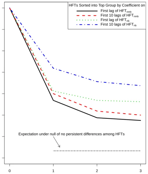
One simple way to look at consistency is to look at the probability an HFT in the highest correlation group remains in that group in future months. Figure5 plots the probability an HFT who is in the highest-correlation group will again be in the highest-correlation group one, two, and three months later. There are three groups, so under the null hypothesis of no persistent difference among HFTs, only 33.3% of the HFTs should still be in the highest-correlation group one month after the sort. In fact, for all sort methods, between 57% and 72% of the HFTs are still in the highest-correlation group one month later. Similarly, in months two and three, more HFTs are still in the high group than would be the expectation under the null hypothesis of no persistence.
Another way to examine persistence is to compare post-sort month coefficients for the three HFT groups. Table5 reports post-sort month coefficients for these groups. The left set of columns is for when the HFT variable is net marketable buying, and the right set is for when the HFT variable is net buying. The top group of rows examines the persistence of the coefficient on the first lag of the HFT variable,γd,t,1. When the HFT variable is net marketable buying, the averageγd,t,1 for the highest-correlation group is 0.024, compared to -0.005 for the lowest-correlation group. Both the Newey and West (1994) p-value and non-parametric rank sum p-value indicate this difference is significantly different from zero. The left group of columns in the middle rows of Table 5 show results using ten lags of HFTs’ net marketable buying. As was the case for the test using just the first lag, the difference between the highest and lowest-correlation groups is significantly different from zero. The right group of columns in Table5report tests using HFTs’ net buying. Results from these tests are the same as for the net marketable buying tests. Finally, the bottom rows show the sum of HFT coefficients when the VAR is extended to 30 lags, and the results are similar. Whether one looks at coefficients on the first lag, first ten lags, or first 30 lags of HFT net marketable buying or net buying, there are persistent differences between the highest and lowest-correlation HFT groups. These results indicate that some HFTs’ trades are consistently more strongly correlated with future non-HFT order flow.
Having split HFTs into groups, I revisit the question of who provides liquidity to HFTs’ mar-ketable trades when they buy or sell a stock aggressively. Prior results aggregating all HFTs showed
that liquidity mostly came from non-HFTs. But perhaps certain HFTs are consistently on the other side of these trades. Panel B in Figure 3 examines cumulative HFT net buying with HFTs split by the coefficient on the first lag of their net marketable buying in the 10-lag regression. The sort is now on net marketable buying aggregated among HFTs in the High group. If HFTs in the Mid orLow groups consistently provide liquidity to the High HFTs, then their net buying should be negative in the second when High HFTs are buying stocks with marketable orders. However, Mid and Low group HFTs are actually slight net buyers in the sort second when High HFTs buy aggressively (and vice versa for theSell portfolio).
Next, Table 6 examines whether marketable trades from HFTs who are skilled at predicting order flow (those in the High group) also forecast larger returns. HFTs are again split into three groups using the methodology from Table 5. Then, trades are aggregated among HFTs in each group, resulting in one time-series of aggregated trades for each HFT group. Returns are then alternately regressed on ten lags of each aggregate HFT series, controlling for ten lags of returns and non-HFT net marketable buying. Thus, the regressions identify the HFT groups’ ability to forecast returns that is independent of information in past returns and non-HFT order flow. For brevity, I only report results for the split on the first lag of HFT net marketable buying in the 10-lag regression.
The results indicate marketable trades from HFTs who are skilled at predicting order flow are better at predicting returns. Coefficients on the first three lags of HFT net marketable buying in the High HFT regressions are 0.0328, 0.0210, and 0.0160, compared to 0.0268, 0.0160, and 0.0125 in the Low group. Both the means and medians of the two coefficient time-series are significantly different from each other, as are the differences in the sum of all 10 lags. These findings are consistent with HFTs in the High group being more skilled at predicting short-term returns.
3.5 Are non-HFTs’ trades more predictable when they are impatient?
Non-HFTs have an incentive to disguise their order flow from HFTs. But as the ITG quote on page 3 highlighted, there is a tradeoff between disguising order flow and trading a large position quickly. It follows that non-HFT order flow may be more predictable when they are impatient. This section tests the hypothesis by comparing VAR estimates from normal times to estimates from times when non-HFTs are hypothesized to be impatient. The VAR is the same as in Section3.1. I focus
on the equation where the dependent variable is non-HFT net marketable buying. If HFTs are doing relatively more anticipatory trading, then I expect larger positive coefficients on the lagged HFT imbalance variables. I examine several times when I expect non-HFTs to be impatient: at the market open and close, on days with high volume or high trade imbalances, and when trading illiquid stocks.
A non-HFT may be impatient at the open if they received an overnight signal (e.g., news) and are concerned other investors either already have or will soon receive the same signal. Similarly, investors near the close may have private information about an end-of-day news announcement. Or they may be facing a liquidity shock that needs to be funded before the close. I use the first and last half hour of the trading day as the opening and close periods. The control period is the rest of the day.
High volume or imbalance days are likely days when certain investors are trading large positions. And it is harder to hide with noise traders when trading a large position. Thus I compare stock days with high volume or a high value of the absolute net marketable buying imbalance to other days. Inspired by Gervais, Kaniel, and Mingelgrin (2001), I classify a day as high volume or high imbalance if the volume/imbalance is among the top 10% of days the past month (i.e., rank relative to prior 19 trading days is 19 or 20).
The motivation for examining illiquid stocks is similar to the intuition for volume and imbal-ances. If non-HFTs do not perfectly scale position sizes relative to liquidity, then in illiquid stocks, their trades will be proportionately larger and thus harder to hide. I identify illiquid stocks as those with wide bid-ask spreads or wide relative spreads (=Bid-Ask Spread÷Bid-Ask Midpoint). Relative spreads account for a $0.01 spread implying different levels of liquidity for a $10 stock and a $100 stock.
Table 7 shows that non-HFT trade predictability is reliably stronger at the market open, on high volume days, and in illiquid stocks. Both the coefficient on the first lag of HFT net marketable buying and the sum of all ten lag coefficients are significantly higher at these times non-HFTs are expected to be impatient. For comparison, the sum of all ten lag coefficients is 0.0076 higher at the open than during the middle of the day, 0.0086 higher on high-volume days than other days, 0.0087 higher in stocks with wide versus narrow quoted spreads, and 0.0046 higher in stocks with wide versus narrow relative spreads. On high imbalance days, the first and sum of all ten coefficients are
also higher than other days, but thet-statistics for the differences with other days are not quite as strong (2.13 and 2.10). The one test that does not go as predicted is the test examining trading near the close. Predictability near the close is weaker than the middle of the day, perhaps because HFTs do not want to build an inventory position they cannot unwind before the end of the day. Overall, the evidence is consistent with HFTs having an easier time anticipating order flow when non-HFTs are more constrained when trying to disguise their trades.
4
Alternative explanations
While the anticipatory trading hypothesis predicts that HFT liquidity demand will be positively correlated with future non-HFT liquidity demand, there are other possible explanations. Any signal that HFTs and non-HFTs separately observe and then trade on could result in HFT liquidity demand positively forecasting non-HFT liquidity demand, particularly if HFTs react faster. This contrasts with anticipatory trading, in which the HFT does not directly observe the same signal as the non-HFT but instead infers it from the non-HFT’s trading activity.
It is difficult to completely rule out this alternative, because it is not possible to fully examine all inputs to HFT and non-HFT trading processes. Nevertheless, if the relation between HFT and non-HFT trading is still strong after accounting for the most likely signals they would both utilize in close succession, then it makes this correlated signal explanation less probable. To examine the issue, this section explores the two most likely signals HFTs and non-HFTs could both be reacting to: news and past returns. It then evaluates whether the results could be caused by another correlated signal explanation—trader misclassification.
4.1 Are HFTs simply reacting faster to news?
Reacting to news faster than other investors is an important HFT skill and plausible explanation for HFT marketable trades leading non-HFT marketable trades (Ye, Yao, and Gai 2013, Foucault, Hombert, and Rosu 2016).
Alternative Hypothesis 1 If HFT trades lead non-HFT trades because HFTs are reacting faster to firm news, then the lead-lag relationship should go away after excluding days with firm news.
News days are identified using a comprehensive set of events: days when an article about the firm is published, an analyst covering it changes their earnings forecast or investment recommendation, management provides new guidance, the firm files an SEC Form 8-K indicating a material event, or the absolute value of the stock’s market-adjusted return is large. The news articles come from Factiva, data for analysts and guidance from Thomson IBES unadjusted detail files, and 8-Ks from the SEC EDGAR website.12 The news article, analyst, guidance, and 8-K events cover the most plausible public news signals HFTs and non-HFTs would both observe. Factiva for example contains articles from over 35,000 sources, including most major newswires, newspapers, and magazines such as The New York Times,Wall Street Journal, Dow Jones Newswire, and Reuters.13 Nonetheless, it is possible HFTs and non-HFTs respond to a signal that is not in one of these databases. The return-based news day measure addresses this concern. If there is an unobserved news event, trading on the signal will affect the stock price. Thus, examining trading after excluding days with absolute market-adjusted returns greater than relatively small thresholds (1%, 0.5%, and 0.25%) minimizes the chance any observed pattern is caused by unobserved news events.
Table 8 tests the news hypothesis using the Table 3 VAR estimated on days when there is no news about the firm. The table shows the positive correlation between non-HFT and lagged HFT net marketable buying still exists after excluding news days.
The first row shows estimates for the full sample, while subsequent rows show the effects of excluding various types of news days. For the news article, analyst, guidance, and 8-K events, the table shows results excluding the news day and also from five days before to five days after the event. The extended +/− 5-day window excludes days that might be contaminated if the news
leaks through private channels before or after the official announcement. The extended window is unneccessary for the return tests, because the return filter already excludes days with information leakage regardless the proximity to public news announcements.
In the Factiva exclusion tests, all coefficients on lagged HFT trading are positive and significant. Additionally, the sum of the first ten lag coefficients is not significantly different from the full sample. In the IBES, 8-K, and return exclusion tests, the first lag coefficients are not significantly different from zero. However, coefficients on lags two and three and the sum of the first 10 are all
12See theSEC websitefor events that trigger 8-Ks. Data is from Phua, Tham, and Wei (2018).
13 Sample firms are matched to articles using IDs Factiva embeds in articles. See Tetlock, Saar-Tsechansky, and
positive and significant. The sum of the first 10 lag coefficients is smaller than the full sample for some of these tests. But the test with the biggest difference is still within 25% of the full-sample estimate.
The final test is the most restrictive. It excludes any day meeting any of the news day definitions. When only the actual news day is removed, coefficients on all three individual lags and the sum of the first ten are all positive and significant. The version using the +/− 5-day window is extremely
restrictive, removing all but 835 of the 23,071 stock days in the full sample. With the extended window, the coefficients on the first three lags are positive, though only the second is significantly different from zero. Looking at the sum of the first ten coefficients provides more power in the limited sample. This sum is positive and significantly different from zero, and the difference with the full sample is not significantly different from zero.
These results show HFT net marketable buying still positively forecasts non-HFT net marketable buying on days without news.
4.2 Is the explanation non-HFTs and HFTs both chase price trends?
Another hypothesis for why HFT trading leads non-HFT trading is that non-HFT trading has a sim-ple predictable relationship with past returns. Section3.1showed HFTs and non-HFTs both chase short-term price trends with their marketable trades. It is possible HFT trades predict non-HFT trades because they are both reacting to lagged returns, except HFTs react faster. Additionally, with non-HFTs following trend-chasing strategies, another possibility is purchases by HFTs could cause future non-HFT buying through their effect on returns.
Alternative Hypothesis 2 If HFT net marketable buying leads non-HFT net marketable buying because non-HFTs chase past price trends, then there should be no correlation between HFT and non-HFT trading after controlling for lagged returns.
This alternative hypothesis is addressed by the VAR in Table3. The coefficients in regressions of non-HFT net marketable buying on HFT net marketable buying are positive controlling for lagged returns. HFT trades may cause some non-HFT trend chasing through their effect on returns, but it is not sufficient to explain the lead-lag correlation between HFT and non-HFT trading.
4.3 Are HFT trades forecasting misclassified HFT trades rather than true non-HFT trades?
Finally, it is possible HFT trading predicts non-HFT trading because some HFT trades are misclas-sified. Misclassification can occur if an HFT routes orders through brokers that handle non-HFT orders, such as Goldman Sachs and Morgan Stanley (Brogaard, Hendershott, and Riordan 2014). The problem with misclassification is that HFT trading is serially correlated. This serial correlation could be caused by some HFTs being slower or by trade splitting. Either way, if you take some of these later HFT trades and throw them into the non-HFT bucket, then current HFT trading will forecast those later misclassified trades. Consequently, misclassification could lead to an erroneous conclusion that HFT trades were forecasting non-HFT trades.
To see how HFT trades would forecast misclassified trades, you can look at how HFT trading forecasts itself. If correctly classified HFT trades are representative of misclassified trades, then the predictability of correctly classified trades should be proportional to that of misclassified trades. For example, a 100 share purchase by correctly classified HFTs might forecast that correctly classified HFTs purchase 20 shares 5 seconds from now and 10 shares 10 seconds from now. If misclassified trade predictability is proportional, then misclassified HFTs might purchase half those amounts 5 and 10 seconds from now. The essential idea is that the decay in predictability will be approximately the same. Importantly, the above hypothesis can be true even if correctly classified trades are not entirely representative of misclassified ones. It is only necessary that the later correctly classified HFT trades that generate the serial correlation are representative of later misclassified trades.
We can make additional predictions under the assumption that most HFT trades are correctly classified. This is a reasonable assumption given NASDAQ attributes roughly 40% of its dollar volume to the HFTs they identified. If correctly classified HFT trades account for the majority of HFT trades, then HFT trading should predict itself more than it predicts non-HFT trading. This is because misclassification implies non-HFT trading is a noisy HFT proxy, so lead-lag correlations should be attenuated relative to a sample with no noise (i.e., the correctly classified HFT trades).
Alternative Hypothesis 3a Misclassification implies the decay in the correlation between non-HFT trading and lagged non-HFT trading is proportional to the decay in the correlation between non-HFT trading and lagged values of itself.
Alternative Hypothesis 3b Misclassification implies HFT trading should forecast itself more strongly than non-HFT trading.
Figure 6 tests the misclassification hypotheses by comparing the VAR coefficients on HFT net marketable buying in Table 3. The dark red line plots coefficients from the regression where the dependent variable is HFT net marketable buying, while the light blue line is for the regression where the dependent variable is non-HFT net marketable buying. The VAR regression coefficients are standardized, so to facilitate comparison they are transformed to show the number of shares change in the dependent variable for a 100 share change in HFT net marketable buying.14 The y-axis is capped to zoom in on higher lags.
First, the figure shows the decay of the HFT to lagged HFT correlation is faster than the decay of the non-HFT to lagged HFT correlation. Using the VAR with 10 lags, Panel A shows coefficients for the first few lags are much higher when HFT net marketable buying is the dependent variable (dark red lines) than when non-HFT net marketable buying is the dependent variable (light blue lines). However, as the lags increase, the coefficients when HFT net marketable buying is the dependent variable drop steadily, while the coefficients when non-HFT net marketable buying is the dependent variable remain comparatively stable. This finding contradicts Alternative Hypotheses3a.
Second, HFT net marketable buying predicts non-HFT net marketable buying better than itself at higher lags. This conflicts with Alternative Hypothesis 3b. Specifically, after seven lags, the HFT coefficient is actually bigger in the regression where the dependent variable is non-HFT net marketable buying. The coefficients in Panel A imply a 100 share increase in HFT net marketable buying ten seconds ago is associated with a 0.066 share increase in HFT net marketable buying, compared to a 0.244 share increase in non-HFT net marketable buying. Using the VAR with 30 lags, Panel B shows the coefficient in the HFT regression is roughly zero by the fifteenth lag, while the coefficient in the non-HFT regression remains positive and significantly different from zero even after 30 lags.
These findings are inconsistent with the misclassification explanation. The simpler explanation is that HFT marketable trades are mostly forecasting correctly classified non-HFT marketable
14For example, the lag 1 HFT coefficient in the non-HFT regression in Table3is 0.0007. Table1shows the mean
standard deviations of HF TN MB (80) and non-HF TN MB (125). The coefficient in terms of a 100 share change in
trades, especially when looking 10 seconds or more into the future.
5
Relation to inventory management
Order anticipation typically comes up in the context of speculation. But being able to anticipate order flow is also useful for HFT market makers managing their inventory risk. Consider a market making HFT who acquires a short position in a stock by selling to liquidity demanding non-HFT buyers. If the HFT subsequently realizes these non-HFT purchases will continue and push prices up, then the HFT can avoid a loss by exiting the short position quickly with a marketable buy order. In this scenario, the HFT buys ahead of non-HFTs to get out of a losing position.
Inventory management and speculation have different implications for how HFTs’ marketable buying is related to existing positions. Marketable trades that reverse existing positions are consis-tent with inventory management.15 Speculation is consistent with the other leg of a marketable pur-chase occuring beforehand or afterwards, though a common expectation is to see a non-marketable sale afterward.
The NASDAQ data does not contain position information. But HFT positions can be estimated by cumulating their net buying across all NASDAQ trades. A downside to this method is that relying on data from a single exchange means it misses position changes caused by trades on other venues (Menkveld 2013, Reiss and Werner 1998). In particular, if an HFT purchases a share of GE on NASDAQ and sells the share on the NYSE, they will appear to be long one share of GE in the NASDAQ data when they actually have no position. Nevertheless, the estimates are informative.
Figure 3 Panel A plots cumulative HFT net buying for the first and tenth net marketable buying decile portfolios. The portfolios are the same as in Figure 1, except the plotted variable is net buying instead of net marketable buying.
If HFTs’ marketable purchases in the sort period are unwinding short inventory positions ac-cumulated over the prior 30 seconds, then the solid line indicating cumulative net buying for decile ten (stocks HFTs buy aggressively in second 0) should be falling in the pre-sort period. However, net buying for decile 10 is slightly increasing in the 30 seconds before the sort. Similarly, inventory management implies the dotted line showing cumulative net buying for decile one (stocks HFTs sell
15For research on inventory management by NYSE specialists, see Hasbrouck and Sofianos (1993), Hendershott