Context Models For Web Search Personalization

Context Models For Web Search Personalization

Maksims N. Volkovs

[email protected]

ABSTRACT

We present our solution to the Yandex Personalized Web Search Challenge. The aim of this challenge was to use the historical search logs to personalize top-N document rank-ings for a set of test users. We used over 100 features ex-tracted from user- and query-depended contexts to train neural net and tree-based learning-to-rank and regression models. Our final submission, which was a blend of sev-eral different models, achieved an NDCG@10 of 0.80476 and placed 4’th amongst the 194 teams winning 3’rd prize1_.

1.

INTRODUCTION

Personalized web search has recently been receiving a lot of attention from the IR community. The traditional one-ranking-for-all approach to search often fails for ambiguous queries (e.g. “jaguar”) that can refer to multiple entities. For such queries, non-personalized search engines typically try to retrieve a diverse set of results covering as many possible query interpretations as possible. This can result in highly suboptimal search sessions, where web pages that the user is looking for are very low in the returned ranking.

In many such cases previous user search history can help resolve the ambiguity and personalize (rank) returned re-sults to user-specific information needs. Recently, a number of approaches have shown that search logs can be effectively mined to learn accurate personalization models [10, 21, 7, 2, 16], which can then be deployed to personalize retrieved re-sults in real time. Many of these models do not require any external information, and obtain all learning signals directly from the search logs. Such models are particularly effective since search logs can be collected at virtually no cost to the search engine, and most search engines already collect them by default.

To encourage further research in this area Yandex recently partnered with Kaggle and organized the Personalized Web Search Challenge2. At the core of this challenge was a large scale search log dataset released by Yandex containing over 160M search records. The goal of the challenge was to use these logs to personalize search results for a selected subset of test users. In this report we describe our approach to this problem. The rest of the paper is organized as follows, Section 2 describes the challenge data and task in detail. Section 3 introduces our approach in three stages: (1) data

1_{Top team “pampampampam” was from Yandex and did not}

officially participate in the competition.

2

www.kaggle.com/c/yandex-personalized-web-search-challenge

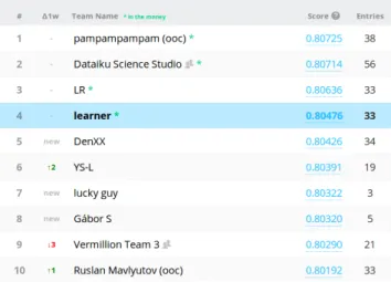
Figure 1: Final leaderboard standings, our team “learner” placed 4’th amongst the 194 teams (261 users) that participated in this challenge.

partitioning, (2) feature extraction and (3) model training. Section 4 concludes with results.

2.

CHALLENGE DESCRIPTION

In this challenge Yandex provided a month’s (30 days) worth of search engine logs for a set of users U =

{u1, ..., uN}. Each useruengaged with the search engine by

issuing queriesQu={qu1, ..., quMu}. Queries that were

is-sued “close” to each other in time were grouped into sessions. For each queryquthe search engine retrieved a ranked list of

web pages (documents)Dqu ={dqu1, ..., dquKqu}, returning

it to the user. User then scanned this list (possibly) click-ing on some documents. Every such click is recorded in the logs together with time stamp and id of the document that was clicked. Only the top ten documents and their clicks (if any) were released for each query soKqu = 10∀qu. For

privacy reasons, very little information about queries and documents was provided. For queries, only numeric query id and numeric query-term ids were released. Similarly, for documents, only numeric document id and corresponding domain id (i.e. facebook.com for facebook pages) were re-leased.

Clicks combined with dwell time (time spent on a page) can provide a good indication of document relevance to the user. In particular, it has been consistently found that longer dwell times strongly correlate with high relevance

Table 1: Dataset statistics Unique queries 21,073,569 Unique documents 70,348,426 Unique users 5,736,333 Training sessions 34,573,630 Test sessions 797,867 Clicks in the training data 64,693,054 Total records in the log 167,413,039

leading to the concept ofsatisfied(SAT) clicks – clicks with dwell time longer than a predefined threshold (for example 30 seconds) [10, 21, 7]. Most existing personalization frame-works assume that documents with SAT clicks are relevant and use them to train/evaluate models.

This competition adopted a similar evaluation framework where each document was assigned one of three relevance labels depending on whether it was clicked and click dwell time length. For privacy reasons dwell time was converted into anonymous “time units” and relevance labels were as-signed according to the following criteria:

• relevance 0: documents with no clicks or dwell time strictly less than 50 time units

• relevance 1: documents with clicks and dwell time between 50 and 399 time units

• relevance 2: documents with clicks and dwell time of at least 400 time units as well as documents with last click in session

Using above criteria, a set of relevance labels Lqu =

{lqu1, ..., lquKu} (one per document) can be generated for

every issued query. Note that these relevance labels are personalized to the user who issued the query and express his/her preference over the returned documents. Given the relevance labels, the aim of the challenge was to develop a personalization model which would accurately re-rank the documents in the order of relevance to the user who issued the query.

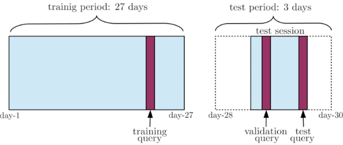
To ensure fair evaluation the data was partitioned into training and test sets. Training data consisted of all queries issued in the first 27 days of search activity. Test data con-sisted of queries sampled from the next 3 days of search activity. To generate the test data one query with at least one relevant (relevance >0) document was sampled from 797,867 users resulting in a fairly large test set with almost 800K queries and 8M documents. In order to simulate real-time search personalization scenario, all search activity after each test query was removed from the data. Furthermore, to encourage discovery of medium and long term search pref-erence correlations all sessions except those that contained test queries were removed from the 3 day test periods. A diagram illustrating data partitioning is shown in Figure 2, and full dataset statistics are shown in Table 1.

All submissions were required to provide full document rankings for each of the 797,867 test queries and were eval-uated using the Normalized Discounter Cumulative Gain (NDCG) [11] objective. Given a test query qu with

doc-umentsDqu and relevance labelsLqu, NDCG is defined by:

NDCG(π,Lqu)@T = 1 GT(L) T X i=1 2L(π−1(i))−1 log2(i+ 1) (1)

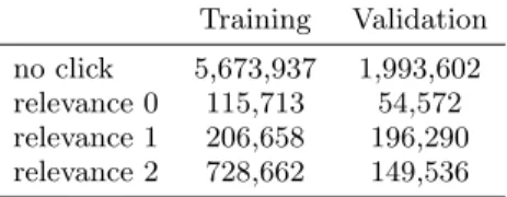
Table 2: Document relevance distribution for train-ing and validation sets.

Training Validation no click 5,673,937 1,993,602 relevance 0 115,713 54,572 relevance 1 206,658 196,290 relevance 2 728,662 149,536

Here π : Dqu → {1, ..., Mu} is a ranking produced by the

model mapping each document dquj to its rank π(j) = i,

and j = π−1(i). L(π−1(i)) is the relevance label of the document in position i in π, and GT(L) is a normalizing

constant. Finally,T is a truncation constant which was set to 10 in this challenge.

As commonly done in data mining challenges, test rele-vance labels were not released to the participants and all submission were internally evaluated by Kaggle. Average NDCG@10 accuracies for approximately 50% of test queries were made visible throughout the challenge on the “public” leaderboard while the other 50% were used to calculate the final standings (“private” leaderboard).

3.

OUR APPROACH

In this section we describe our approach to this challenge. Before developing our models we surveyed existing work in this area and found that most personalization methods can be divided into three categories: heuristic, feature-based and user-based. Heuristic methods [9] use search logs to com-pute user-specific document statistic, such as the number of historical clicks, and then use this statistic to re-rank the documents. Since it is often difficult to know which statis-tic will work best, feature-based models [2, 18, 16] extract a diverse set of features used as input for machine learning methods that automatically learn personalization models. Note that while features are extracted separately for every user-query-document triplet, the same model is used to re-rank documents for all users.

Finally, user-based methods [17, 15, 20] as the name sug-gests, learn separate models for each user. Some of these models use collaborative filtering techniques to infer la-tent factors for users and documents [17, 15], while others adapt learning-to-rank models by incorporating user-specific weights and biases [20].

User-based models allow the highest level of personaliza-tion but require extensive user search history and/or side information about queries and documents (such as top-ics, document features etc.). Given the sparsity of our data (70M unique documents in 160M records) and lack of user/query/document information we opted to use the feature-based approach. In the following sections we de-scribe in detail all the components that were necessary to create a feature-based model, namely data partitioning, fea-ture extraction and learning/inference algorithms.

3.1

Dataset Partitioning

We begin by describing our data partitioning strategy. Properly selected training/validation datasets are crucial to the success of any data mining model. Ideally we want these datasets to have very similar properties to the test data. To achieve this we carefully followed the query sampling

proce-Figure 2: Diagram showing data partition and training/validation/test query selection (in red) for a single

user. Training query was always selected to be the last query in training period with at least one relevant (relevance>0) document. Similarly, validation query was always selected to be the last query in test session with at least one relevant document. Test query was given a priori and was the last query in test session.

dure (described in Section 2) used by competition adminis-trators to select test queries.

For each user we first sorted all sessions by day (lowest to highest) randomly resolving ties since exact timestamps were not available. We then selected the last query in the 27 day training period with at least one relevant (relevance>

0) document as training query. Similarly, last query in test session with at least one relevant document was selected for validation. This selection process is shown in Figure 2.

The motivation behind choosing these specific queries was 3-fold. First, since features can only be extracted from queries issued before the given query, we need to choose queries with as much historical data as possible. Select-ing queries at the end of trainSelect-ing period and test session ensures maximum historical data. Second, there could be a large time gap between the end of training period and test session, and during that time the user’s search needs and preferences could change significantly. To capture this we need both training and validation queries to be as close as possible to test ones. However, since many test session did not have enough data to select two queries, only validation query was sampled from this session. Finally, only select-ing queries with at least one relevant document ensures that their is sufficient training signal for learning-to-rank models. Training objectives in these models are often order-based and thus require at least one relevant document.

Applying this procedure to each of the 797,867 test users and removing users that did not have enough data, resulted in 672,497 training and 239,400 validation queries. Once the data was partitioned relevance labels were computed for all documents in both training and validation queries using the criteria outlined in Section 2. Table 2 shows relevance label distribution across documents in both sets. From this table we see that the majority of documents with clicks have relevance label 1 or 2. This suggests that once the user clicks on a document (s)he tends to spend “significant” amount of time going through the content of that document. It can also be seen that validation relevance distribution is similar to training one with the exception that training data has considerably more highly relevant (relevance 2) documents.

3.2

Feature Extraction

After partitioning the data and computing relevance la-bels we proceeded to feature extraction. Our aim was to extract features for every training, validation and test user-query-document triplet (u, qu, dqu). As mentioned above,

the available log data provided very little information about individual queries and retrieved documents. For queries, we only had access to term vectors with individual terms con-verted to numeric ids. Similarly, for documents we only had access to their domain ids and base ranking generated by the Yandex search engine. In this form the personalization problem is similar to collaborative filtering/ranking where very little information about items and users is typically available. Neighborhood-based models that extract features from similar items/users have been shown to consistently perform well in these problems and were an essential part of the Netflix prize winning solution [13]. In search per-sonalization, ranking models learned on features extracted from user’s search neighborhoods (historical sessions, queries etc.) have also been recently shown to perform well [2, 16, 18]. Inspired by these results we concentrated our efforts on designing features using historical search information in the logs.

We began by identifying several “contexts” of interest. Here, contexts are analogous to user/item neighborhoods in collaborative filtering, and contain collections of queries that have some relation to the target user-query-document triplet for which the features are being extracted. Formally we define context as:

Definition 1.

Context C = {{q1, ..., qM},{Dq1, ...,DqM},{Lq1, ...,LqM}}

is a set of queries with corresponding document and rele-vance label lists.

Given a user-query-document triplet (u, qu, dqu), we

pri-marily investigated two context types: user-related and query-related. For user-related contexts we considered all queries issued by u before qu and partitioned them into 2

contexts - repetitions of qu and everything else. The

ra-tionale behind this partitioning is that past instances ofqu

forqu[9], and should be processed separately. In addition

to historical queries fromu, we computed context from all instances ofqu issued by users other than u. This context

provides global information on user preferences for docu-ments inqu, and can be useful when little information from uis available.

For each of these contexts we computed features on both document and domain levels. To use domains we simply sub-stituteddqu with its domain and replaced document lists in

each context with domain lists. Given that multiple docu-ments can have the same domain we expect domain features to be less precise. However, domain data is considerably less sparse (∼70M unique documents vs∼5M unique domains) and can thus provide greater coverage. Using both docu-ment and domain lists we ended with a total of 6 contexts:

• C1: all repetitions ofqubyu

• C2: same asC1 but with domain lists • C3: all queries other thanquissued byu

• C4: same asC3 but with domain lists • C5: all repetitions ofquby users other thanu

• C6: same asC5 but with domain lists

In this form our contexts are similar to “views” explored in [2]. The main difference between the two is that views are user-specific whereas contexts can include any set of queries including those from other users. Note that we also do not apply any session-based partitioning within the contexts and all queries are simply aggregated together. Throughout the challenge we experimented with several session-related con-texts (current session vs past sessions) but did not find them to give significant improvement.

After specifying the contexts we defined a total of 20 context-dependent features described in detail in Appendix A. Most of these features aim to capture how frequently

dquwas shown/clicked/skipped/missed in the given context.

The features also try to account for the rank position ofdqu

across the context and similarity between qu and context

queries. Query similarity featuresg4 -g9 (see Appendix A)

are only relevant when queries other thanqu are included

in the context, and are thus only extracted for contextsC3

andC4. All together, we computed 20 features forC1,C2, C5,C6 and 16 features forC3,C4 giving us a total of 112

context features. In addition to these features, we added rank ofdqu returned by the search engine as the 113’th and

final feature.

All of the 20 context features only require simple opera-tions and are straightforward to implement. Similarly, con-textsC1-C4are readily available in the log data and can be

easily extracted. ContextsC5andC6on the other hand, are

trickier to compute efficiently since they require access to all instances of a particular query. To calculate these we created an inverted hash map index mapping each unique query id to a table storing all occurrences of this query id in the logs with corresponding document, domain and relevance label lists. For any query a single lookup in this index was then re-quired to compute features for every document returned for that query. The full features extraction for training, valida-tion and test queries (∼1.7M queries with 17M documents) implemented in Matlab took roughly 7 hours on a Thinkpad W530 laptop with Intel i7-3720QM 2.6 GHz processor and 32GB of RAM.

3.3

Learning and Inference

We trained several learning-to-rank and regression models on the extracted feature data. For learning-to-rank mod-els we used RankNet [4], ListNet [5] and a variation of BoltzRank [19]. Given the success of tree-based generalized gradient boosting machines (GBMs) on recent IR bench-marks such as the Yahoo!’s Learning To Rank challenge [6], we also experimented with state-of-the-art GBM learning-to-rank model LambdaMART [3]. We omit the details of each model in this report and refer the reader to respective papers for detailed descriptions.

For pairwise RankNet model we experimented with var-ious ways to extract pairwise preferences from click data. Specifically, many studies have shown that users scan re-turned results from top to bottom [12, 14] so documents ranked below the bottom-most click were likely missed by the user. It is thus unclear whether we should use those documents during training and if so what relevance should they be assigned. Skipped documents (i.e. those above the bottom-most click) on the other hand, were clearly found not relevant by the user. However, it is also unclear whether they should be assigned the same relevance label 0 that is given to clicked documents with low dwell time. Intuitively, it seems like click is a stronger preference signal than skip even if dwell time after that click is low.

To validate these hypotheses, we used a 1-hidden layer neural net implementation of RankNet and trained it on different preference targets extracted from clicks. We exper-imented with several variations of the cascade click model [12] as well as various relevance re-weightings. Across these experiments the best results were obtained by simply set-ting relevance of skipped and missed documents to zero and training on all the available data. These results, although somewhat surprising, can be possibly explained by the fact that this assignment matches the target one used in NDCG for model evaluation. In light of these results we used the

{0,1,2}relevance assignment in all subsequent experiments.

4.

RESULTS

In this section we describe the main results achieved by our models. Throughout the experiments we consistently found that performance (gains/losses) on our in house val-idation set closely matched the public leaderboard. At the end of the competition we also saw that public and private leaderboard results were very consistent. In this report we thus concentrate on private leaderboard NDCG scores since these scores were used to compute the final standings. We note that these results were only available after the com-petition ended so it was impossible to directly optimize the models for this set.

At the beginning of the competition, before applying so-phisticated machine learning methods, we created a simple heuristic-based model that re-ranked documents based on their total historical relevance. Specifically, for every test documentdqu we computed featureg1(see Appendix A)

us-ing all previous instances of qu issued by u (context C1).

We then re-ranked documents by g13 using original

rank-ing to resolve ties. This model produced an NDCG@10 of 0.79754 shown in Table 3 (“re-rank by hist relevance”) which is a relative improvement of 0.0062 over the baseline

3_{We also experimented with featuresg}

2-g4but foundg1 to

Table 3: Private leaderboard average NDCG@10 re-sults. Only results for the best model of each type are shown.

Model NDCG@10 default ranking baseline 0.79133 re-rank by hist relevance 0.79754 regression (NN) 0.80315 learning-to-rank (NN) 0.80324 LambdaMART 0.80330

aggregate average 0.80378 aggregate RankNet 0.80476

non-personalized ranking produced by Yandex’s search en-gine. This submission would have placed 32’nd on the final leaderboard.

After verifying that personalization from logs is possible, we proceeded to learning-to-rank and regression models. We trained 1-hidden layer neural net implementations of each model using tanh activation units and varying the number of hidden units in the [10, 200] range. Regression models were optimized with squared-loss objective function. Before learning, all features were standardized to have mean 0 and standard deviation of 1. For each model we used mini-batch learning with batch size of 100 queries (1000 documents), processing each query in parallel. Parallel processing allowed us to fully train these models on all of the available train-ing data in several hours ustrain-ing the same Thinkpad W530 machine.

Results for best neural net (NN) regression and learning-to-rank models are shown in Table 3. From the table we see that both models significantly improve NDCG@10 with relative gains of up to 0.0118 over the baseline ranking. We also see that regression models perform similarly to learning-to-rank ones with learning-learning-to-rank only providing marginal gains. For both types of models we found that neural nets with 50 - 100 hidden units performed the best. Moreover, for learning-to-rank we found that RankNet performed slightly better than other ranking models but the difference was not significant (less than 0.0001).

Best result for LambdaMART is also shown in Table 3. We used publicly available RankLIB library [8] to run Lamb-daMART. Training LambdaMART took a very long time (on the order of days) and used close to 25GB of RAM. We were thus unable to properly validate/tune all the hy-per parameters such as the number of leaves and learning rate. This possibly explains the marginal performance of this model as seen from Table 3, where it is performing com-parably to the neural net models.

4.1

Model Aggregation

For each experiment that we ran throughout the competi-tion we saved models that performed best on the validacompeti-tion set. This gave us ∼30 trained models at the end of the competition. It’s well known that blending improves accu-racy of individual models, and blended solutions have won many data mining competitions including the Netflix chal-lenge [13]. Keeping this in mind we spent the last few days of the competition finding the best blend of the models that we had trained.

Before applying any blending techniques we standardized

the scores produced by each model to have mean 0 and standard deviation 1. After normalization we began with a simple baseline that averaged all the available scores. This baseline obtained an NDCG@10 of 0.80378 and is shown in Table 3 (“aggregate average”). While this is an improve-ment over the best individual model, the improveimprove-ment is not significant. This can be attributed to the fact that many models in our blending set were considerably weaker than the best model. Consequently, including all of these mod-els in the blend with equal weight significantly affected the overall accuracy. It is thus evident that with many weaker models simple averaging is not optimal and more adaptive techniques are necessary.

One possible solution is to use model-specific weights dur-ing aggregation. Weights are typically chosen to be a func-tion of model’s accuracy and several such funcfunc-tions have have been suggested in literature [1]. However, instead of tuning these weights by hand a more principled and poten-tially more accurate approach is to apply one of the learning-to-rank methods to automatically learn the weights.

We experimented with this approach and began by par-titioning our validation4 set into two subsets. One subset was then used to train a linear RankNet on score outputs of all models in the aggregating set, and the other subset was used for validation. The result for this model is shown at the bottom of Table 3 (“aggregate RankNet”). It produced an NDCG@10 of 0.80476 and was our best submission in this competition placing 4’th on the private leaderboard.

4.2

Analysis of Results

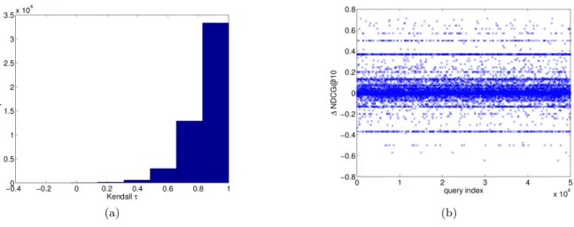
To analyze the effect of personalization we computed Kendall τ correlations between rankings produced by our best model and the non-personalized baseline rankings from Yandex. The plot for randomly chosen 50K validation queries is shown in Figure 3(a). From this figure we see that for most queries τ is above 0.7 indicating that our model is fairly conservative and tends to only re-rank a few doc-uments in the list. However, we also see that a number of queries are very aggressively re-ranked withτ below 0.5.

While aggressive personalization can significantly improve user search experience, it can also lead to dangerous outlier queries where top-N documents are ranked completely out of order. This is further illustrated in Figure 3(a) which shows the difference in NDCG@10 between our model and Yandex’s base ranking for the same 50K queries. From this figure we see that while personalized model improves NDCG for many queries, some queries are also significantly hurt with NDCG drops of over 0.4. This further demonstrates the danger of applying personalization to all queries and emphasizes the need for adaptive strategies that selectively choose which queries should be re-ranked. Moreover, risk minimization (largest NDCG loss across all queries) might be a more appropriate objective for this task since it can produce models with more stable worst-case performance. This, however, is beyond the scope of this paper and we leave it for future research.

5.

CONCLUSION AND FUTURE WORK

In this paper we presented our solution to the Yandex Personalized Web Search Challenge. In our approach search

4_{Note that training set should not be used for aggregation}

(a) (b)

Figure 3: Figure 3(b) shows NDCG@10 difference between our best personalized model and static ranking produced by Yandex for 50K validation queries. Figure 3(a) shows Kendallτ distance histogram for the same 50K queries. Kendallτ is computed between personalized and non-personalized ranking for each query.

logs were first partitioned into user and query dependent neighborhoods (contexts). Query-document features were then extracted from each context summarizing document preference within the context. Models trained on these fea-tures achieved significant improvements in accuracy over non-personalized ranker.

In the future work we plan to explore contexts based on similarqueries/users. Such contexts have been successfully applied in neighborhood-based collaborative filtering mod-els and can potentially be very useful in this domain as well. Both user an query similarities can be readily inferred from the search logs using statistics like issued query overlap for users and document/domain overlap for queries. These con-texts can be particularly useful for personalization of long-tail queries that occur very infrequently in the data and do not have enough preference data.

6.

ACKNOWLEDGMENTS

We would like to thank Yandex for organizing this com-petition and for releasing such an interesting large-scale dataset. We would also like to thank Kaggle for hosting and managing the competition.

7.

REFERENCES

[1] J. A. Aslam and M. Montague. Models for metasearch. InSIGIR, 2001.

[2] P. N. Bennett, R. W. White, W. Chu, S. T. Dumais, P. Bailey, F. Borisyuk, and X. Cui. Modeling the impact of short- and long-term behavior on search personalization. InSIGIR, 2012.

[3] C. J. C. Burges. From RankNet to LambdaRank to LambdaMART: An overview. Technical Report MSR-TR-2010-82, Microsoft Research, 2010. [4] C. J. C. Burges, T. Shaked, E. Renshaw, A. Lazier,

M. Deeds, N. Hamilton, and G. Hullender. Learning to rank using gradient descent. InICML, 2005.

[5] Z. Cao, T. Qin, T.-Y. Liu, M.-F. Tsai, and H. Li. Learning to rank: From pairwise approach to listwise approach. InICML, 2007.

[6] O. Chapelle and Y. Chang. Yahoo! learning to rank challenge overview.Jouranl of Machine Learning Research, 14, 2011.

[7] K. Collins-Thompson, P. N. Bennett, R. W. White, S. de la Chica, and D. Sontag. Personalizing Web search results by reading level. InCIKM, 2011. [8] V. B. Dang. Ranklib.

http://people.cs.umass.edu/~vdang/ranklib.html. [9] Z. Dou, R. Song, and J.-R. Wen. A large-scale

evaluation and analysis of personalized search strategies. InWWW, 2007.

[10] S. Fox, K. Kuldeep, M. Mydland, S. Dumais, and R. White. Evaluating implicit measures to improve Web search. InACM TOIS, 2005.

[11] K. Jarvelin and J. Kekalainen. IR evaluation methods for retrieving highly relevant documents. InSIGIR, 2000.

[12] T. Joachims, L. Granka, B. Pan, H. Hembrooke, F. Radlinski, and G. Gay. Evaluating the accuracy of implicit feedback from clicks and query reformulations in web search.ACM Transactions on Information Science, 2007.

[13] Y. Koren. Factorization meets the neighborhood: a multifaceted collaborative filtering model. InKDD, 2008.

[14] O.Chapelle, D. Metzler, Y. Zhang, and P. Grinspan. Expected reciprocal rank for graded relevance. In Proceeding of the ACM Conference on Information and Knowledge Management, 2009.

[15] F. Qiu and J. Cho. Automatic identification of user interest for personalized search. InWWW, 2006. [16] M. Shokouhi, R. W. White, P. Bennett, and

F. Radlinski. Fighting search engine amnesia: Reranking repeated results. InSIGIR, 2013. [17] J.-T. Sun, H.-J. Zeng, H. Liu, Y. Lu, , and Z. Chen.

CubeSVD: A novel approach to personalized web search. InWWW, 2005.

[18] J. Teevan, S. T. Dumais, and D. J. Liebling. To personalize or not to personalize: Modeling queries

with variation in user intent. InSIGIR, 2008. [19] M. N. Volkovs and R. S. Zemel. BoltzRank: Learning

to maximize expected ranking gain. InICML, 2009. [20] H. Wang, X. He, M.-W. Chang, Y. Song, R. W.

White, and W. Chu. Personalized ranking model adaptation for web search. InSIGIR, 2013. [21] K. Wang, T. Walker, and Z. Zheng. Estimating

relevance ranking quality from web search clickthrough data. InSIGKDD, 2009.

APPENDIX

A.

CONTEXT FEATURES

Given user-query-document triplet (u, qu, dqu) and

con-textC we extract a total of 20 context-dependent features

g1 -g20(all missing features are set to 0): • Total relevance for all clicks ondqu inC:

g1= X q∈C X dq∈Dq I[dq=dqu]lq

whereI[x] is an indicator function evaluating to 1 ifx

is true and 0 otherwise

• Average relevance for all clicks ondqu inC:

g2= 1 P q∈C P dq∈DqI[dq=dqu] X q∈C X dq∈Dq I[dq=dqu]lq

• Max/min relevance across all clicks ondqu inC:

g3= arg max{lq|q∈C, dq∈Dq, dq=dqu}

g4= arg min{lq|q∈C, dq∈Dq, dq=dqu}

• Average similarity between qu and all queries in C

wheredqu was clicked:

g5= 1 P q∈Cclicked(dqu,Dq) X q∈C clicked(d,Dq)sim(q, qu)

where clicked(dqu,Dq) = 1 ifdwas clicked inDqand 0

otherwise. sim(q, qu) is similarity betweenqandqu, in

this work we use intersection over union metric applied to query terms.

• Max similarity betweenqu and all queries inC where dqu was clicked:

g6= arg max{sim(q, qu)|q∈C,clicked(dqu,Dq) = 1}

• Average similarity between qu and all queries in C

where dqu was skipped (i.e. dqu was not clicked but

there was at least on click belowdqu):

g7= 1 P q∈Cskipped(dqu,Dq) X q∈C skipped(dqu,Dq)sim(q, qu)

where skipped(dqu,Dq) = 1 if dqu was skipped in Dq

and 0 otherwise.

• Max similarity betweenqu and all queries inC where dqu was skipped:

g8= arg max{sim(q, qu)|q∈C,skipped(dqu,Dq) = 1}

• Average similarity between qu and all queries in C

wheredqu was missed (i.e. all clicks were aboved):

g9= 1 P q∈Cmissed(dqu,Dq) X q∈C missed(dqu,Dq)sim(q, qu)

where missed(dqu,Dq) = 1 ifdquwas missed inDqand

0 otherwise.

• Max similarity betweenquand all queries inC where dqu was missed:

g10= arg max{sim(q, qu)|q∈C,missed(dqu,Dq) = 1}

• Number of timesdqu was shown, clicked, skipped and

missed inC: g11= X q∈C I[dqu ∈Dq] g12= X q∈C clicked(dqu,Dq) g13= X q∈C skipped(dqu,Dq) g14= X q∈C missed(dqu,Dq)

• Number of times dqu was shown in C discounted by

rank: g15= X q∈C 1 r shown(dqu,Dq)

where r shown(dqu,Dq) is rank ofdqu inDq if it was

shown and 0 otherwise. When r shown(dqu,Dq) = 0

the ratio is set to 0.

• Number of times dqu was clicked in C discounted by

rank: g16= X q∈C 1 r clicked(dqu,Dq)

where r clicked(dqu,Dq) is rank ofdqu inDq if it was

clicked and 0 otherwise. When r shown(dqu,Dq) = 0

the ratio is set to 0.

• Max/min rank ofdqu when it was clicked inC

g17= arg max{r clicked(dqu,Dq)|q∈C}

g18= arg min{r clicked(dqu,Dq)|q∈C}

• Number of timesdqu was skipped inC discounted by

rank: g19= X q∈C 1 r skipped(dqu,Dq)

where r clicked(dqu,Dq) is rank ofdqu inDq if it was

skipped and 0 otherwise. When r skipped(dqu,Dq) = 0

the ratio is set to 0.

• Number of times dqu was missed in C discounted by

rank: g20= X q∈C 1 r missed(dqu,Dq)

where r clicked(dqu,Dq) is rank ofdqu inDq if it was

missed and 0 otherwise. When r missed(dqu,Dq) = 0