ORIGINAL ARTICLE
Multi-objective approach for load shedding based
on voltage stability index consideration
R. Kanimozhi
a,*, K. Selvi
b, K.M. Balaji
a aDepartment of Electrical and Electronics Engineering, BIT Campus, Anna University – Tiruchirappalli, Tamil Nadu 620024, India bDepartment of Electrical and Electronics Engineering, Thiagarajar College of Engineering, Madurai, Tamil Nadu, India
Received 30 December 2013; revised 16 August 2014; accepted 4 September 2014 Available online 7 October 2014
KEYWORDS NVSI; Voltage stability; Contingency; Load shedding; Genetic algorithm; Power flow restorability
Abstract In voltage stability analysis, it is useful to assess voltage stability of power systems by means of scalar magnitudes, or indices. Operators can use voltage stability indices to know how close the system to voltage collapse. The voltage stability indices are a powerful tool to identify the weakest bus and critical line. This identification can be used to gain control over devices for voltage stability up to certain level and load shedding is possible if the load keeps on increasing. This paper presents a computationally simple index based load shedding algorithm using weighted sum genetic algorithm where an AC power flow solution cannot be found for the stressed conditions. Minimization of total load shed and sum of New Voltage Stability Index (NVSI) at the selected buses are considered as two objectives of this algorithm to restore the power flow solvability. This is validated in both IEEE 30 bus system and a practical system Tamil Nadu Electricity board (TNEB) 69 bus system in India for considering both heavy loading and (N1) contingency.
ª2014 Production and hosting by Elsevier B.V. on behalf of Faculty of Engineering, Alexandria University.
1. Introduction
Power systems, nowadays are operating under increased stres-ses because of the lack of proper planning for expansion. Due to economic and environmental restrictions, there is no expan-sion of transmisexpan-sion networks with the increase of loads. Interconnected power systems are operated with higher power
transfers between areas but there is little coordination and exchange of on-line information between utilities. And hence, adequate voltage level monitoring system and data exchange is not in place, which becomes pivotal in case of blackouts. In essence, the direct cause for blackouts has been found to be voltage collapse. Enhancement of power system voltage sta-bility has seen extensive research with proposals and successful implementation of some measures such as VAR (Volt Ampere Reactive) compensation, load shedding and active power con-trol. Many earlier works are available for under frequency, under voltage with no solution for power flow equations being suggested.
Optimal steady state load shedding was formulated to minimize the sum of the squares of the differences between
* Corresponding author. Tel.: +91 0431 2407970, mobile: +91 09677477905.
E-mail addresses: [email protected] (R. Kanimozhi),
[email protected](K. Selvi).
Peer review under responsibility of Faculty of Engineering, Alexandria University.
H O S T E D BY
Alexandria University
Alexandria Engineering Journal
www.elsevier.com/locate/aejwww.sciencedirect.com
http://dx.doi.org/10.1016/j.aej.2014.09.005
the connected loads and the generated power. The supplied power was treated as a dependent variable modeled as a function of the bus voltage magnitude[1].
A simple new technique was developed to define the optimum location and the optimum quantity of load to be shed in order to prevent the system voltage from going to the unstable zone using L-indicator index [2]. A method of load shedding was proposed with objective of minimize load shedding in the situation where total generation is less than the total demand by minimizing system loss with the constraints on generator limits and line flow limits[3]. Some of literatures were proposed corrective model or preventive model for load shedding incorporating dynamic analysis to increase loading margin [4]. A new methodology has been developed for optimum load shedding based on Hopfield neu-ral network model for optimization. Minimum Eigen value was used as indicator. A threshold value of this indicator can be assumed for a specific system. Emergency load shedding required if this value fell below the threshold value[5].
Recently many of the researchers proposed many heuristic algorithms to improve for load shedding automation. An opti-mal load-shedding algorithm was developed for undervoltage load shedding using two heuristic methods such as Particle Swarm Optimization (PSO) and Genetic Algorithm (GA)[6]. A computational algorithm for minimum load shedding at selected load buses was developed using Differential Evolution (DE), Self-adaptive Differential Evolution (SaDE) and Ensemble of Mutation and Crossover Strategies and Parame-ters in Differential Evolution (EPSDE). Developed algorithm accounts inequality constraints not only in present operating conditions (after load shedding) but also for predicted next interval load (with load shedding)[7]. The buses for load shed-ding were selected based on the sensitivity of minimum Eigen value of load flow Jacobian with respect to load shed. A compu-tational algorithm for minimum load shedding was developed using DE [8]. Computational intelligence techniques, due to their robustness and flexibility in dealing with complex non-linear systems, could be an option in addressing this problem. Computational intelligence includes techniques such as artificial neural networks, genetic algorithms, fuzzy logic control, adaptive neuro-fuzzy inference system, and particle swarm optimization. Research in these techniques is being undertaken in order to discover means for more efficient and reliable load shedding. Advantages and drawbacks of these intelligence techniques in load shedding were discussed briefly in[9].
The solution of the power flow problem has received much attention over the last several decades. This is due to its funda-mental importance to power system analysis. However little attention has been focused on how to handle situations where the power flow equations have no real solution. As power systems become more heavily loaded, there will be an increase in the number of situations where the power flow equations have no real solution, particularly in contingency analysis and planning applications. Since these cases can represent the most severe threats to viable system operation, it is important that a computationally efficient technique be developed to both quantify the degree of unsolvability, and to provide optimal recommendations of the parameters to change to return to a solvable solution[10].
Analysis of the power flow feasibility boundary has received considerable attention in the literature. Very few literatures are available to load shed to restore power flow
solution. A methodology was proposed for identifying the fewest network topological changes (removal of transmission lines) that result in operating point infeasibility, such that the amount of minimum load shedding required for feasible operation is greater than a user-defined threshold [11]. A computationally simple algorithm was developed for studying the load shedding problem in emergencies where an AC power flow solution cannot be found for the stressed system. This algorithm was divided into two sub-problems: restoring solvability sub-problem and improving voltage stability margin (VSM) sub-problem. Linear optimization (LP)-based optimal power flow (OPF) is applied to solve each sub-problem. In restoring solvability sub-problem, rather than taking restoring power flow solvability as direct objective function, the objective function of maximization of voltage magnitudes of weak buses was employed. In VSM sub-problem, the tra-ditional load shedding objective was extended to incorporate both technical and economic effects of load shedding and the linearized VSM constraint was added into the LP based OPF
[12].
The feasible region is the set of points where the power flow equations have a solution and all system values (e.g., line flows, bus voltages) are within their limits. Normally this is the desired operating region for the system. Let the infeasible region be the set of points where the power flow equations have a solution, but where one or more limit is violated. Usually it is possible to operate the system (at least for a while) in this region. Much progress has been made in the development of security enhancement tools to provide control-ler recommendations for moving from the infeasible region back into the feasible region. Denote the feasible and infeasible regions as the power flow solvable region. Lastly, let the unsolvable region be the set of points where the power flow equations have no real solution. In this paper, restoring power flow solvability is pursued through load shedding. The load shed buses are selected based on the NVSI value, i.e., high value of NVSI indicates the weak buses and it needs load shedding to restore power flow solvability and improve voltage magnitudes. The minimization of sum of NVSI and sum of load shed at selected buses are considered as objectives of this algorithm. This multi-objective optimization is implemented through the weighted-sum genetic algorithm.
2. Load shedding algorithm
Load shedding techniques are commonly classified as three types namely conventional, adaptive and computational intel-ligence based load shedding techniques. The drawbacks of the conventional method of load shed are as follows: (i) it does not provide optimum load shedding (ii) and does not deal efficiently with modern and complex power systems.
2.1. Genetic Algorithm (GA) application in load shedding
The Genetic Algorithm (GA) is the global optimization tech-nique for solving non-linear, multi-objective problems [13]. The GA is used for this work, due to its evolutionary nature, least mathematical requirement regarding the problems, capability to solve much more complex problems beyond the scope of conventional methods and suitable for solving multi-objective problems. Since the GA provides greater
flexibility to hybridize with conventional methods and the mer-its of both the GA and the conventional method is utilized to make much more efficient implementations to obtain opti-mized solution[13].
GA also has some application in load shedding problems. GA based algorithm for load shedding using the database which was obtained from a power flow study has been pro-posed and was successfully implemented on the IEEE 30-bus system [14]. The load shedding technique for each bus using GA is proposed in[15]and comparison has been done between GA and PSO techniques which are used to solve generator outage and line outage cases. The results show that in terms of computation time, PSO is faster than GA; the minimum amount of load is shed by GA.
The GA application for minimization of the load shed amount for a single-machine infinite bus was tested by simulat-ing the 12-month load demand for an optimal UFLS (Under Frequency Load Shedding) setting and the results compared with a conventional technique that indicate GA-based technique is feasible and effective in providing optimal load shedding [16]. A GA-based method is utilized to determine the supply restoration and optimal load shedding strategy for distribution networks[17]. The survey which is stated con-cludes that, the GA is global optimization technique for solv-ing non-linear, multi-objective problems and also it ensures minimum amount of load shedding even though taking com-paratively long time to determine the load shedding amount.
2.2. Weighted sum approach in load shedding
One of the special issues in the multi-objective optimization problems is fitness assignment mechanism. Most fitness assign-ment mechanisms can be classified into Pareto ranking based fitness assignment and weighted sum-based assignment. Gen-erally, the main idea of Pareto ranking-based approach is to provide clear classification between non-dominated solution and dominated solution for each chromosome. Different from Pareto ranking based fitness assignment, weighted-sum based fitness assignment is to assign weights to each objective func-tion and combines the weighted objectives into a single objec-tive function. It is easier to calculate the weight-sum based fitness and the sorting process becomes unnecessary. In addi-tion, another characteristic of weighted-sum approach is to adjust genetic search toward the Pareto frontier. For combin-ing weighted objectives into a scombin-ingle objective function, the good fitness values are assigned which solutions near from the Pareto frontier[13].
The load shedding algorithm in this paper is a multi-objec-tive one, the objecmulti-objec-tive function must be carefully chosen, so the evolutionary process could go into the right direction, ‘‘increase the robustness with low cost’’. For a good fit of the objective function with this paper, the method of ‘‘weight-ing coefficients’’ has been chosen. This means, the two objec-tives can be virtually separated, by giving each of them its specific weight in the optimization process, written as
fðx1;x2Þ ¼w1fðx1Þ þw2fðx2Þ ð1Þ
This can be modified to this application as,
fðx1;x2Þ ¼wfðx1Þ þ ð1wÞ fðx2Þ w2 ½0;1 ð2Þ
3. Formulation of load shed optimization problem 3.1. Voltage stability index
A New Voltage Stability Index (NVSI) has been proposed which originates from the equation of a two bus network, neglecting the resistance of transmission line, resulting in appreciable variations in both real and reactive loading[18]. In general, the NVSI formulation connecting bus ‘‘i’’ to bus ‘‘j’’ can be given by NVSIij¼ 2X ffiffiffiffiffiffiffiffiffiffiffiffiffiffiffiffiffiffiffiffiffiffiffi P2j þQ2j r 2QjXV2 i ð3Þ
Variable definition follows.
X: line reactance,
Qj: reactive power at the receiving end,
Vi: sending end voltage,
Pj: real power at the receiving end.
The value of NVSI must be less than 1.00 in all transmis-sion lines to maintain a secure system. With this index infor-mation, we can rank load bus in decreasing order, and select the buses with large component of NVSI as weak buses to per-form load shedding.
3.2. Objective function
In this paper, power flow solvability is restored through load shedding. Sum of the total active demand reduction and the sum of NVSI values are minimized for select weak buses for load shedding. The fixed weighted sum genetic algorithm is used to minimize the objective function
Min x¼wX LSB i¼1 NVSIþ ð1wÞX LSB i¼1 ðDP0iÞ ð4Þ subject to the following constraints andLSBdenotes load shed buses andDP0i– load shedding at bus i.
3.3. Constraints
The load shedding algorithm is formulated in terms of both active and reactive power parameters. Therefore, the following notations have been adopted.
PG0i – Initial active generation in generator bus i, DPG0i – Active generation variation in generator bus i, PGi – Lower limit of generation in generator bus i,
PD0i– Initial active demand in bus i,
DPD0i – Active demand variation in bus i, QD0i– Initial reactive demand in bus i,
DQD0i– Reactive demand variation in bus i,
DPtotal– Total maximum possible load shedding,
DPmin
0i – Minimum load shedding in bus i,
DPmin
1. The power factor is maintained as the original in every load bus
QD0iDPD0iPD0iDQD0i¼0 8i ð5Þ
2. The load shedding of selected load buses is bounded by the total load shedding.
XLSB i¼1
DP0iDPtotal ð6Þ
3. The load shedding at each selected bus is within the limits
DPmin
0i DP0iDPmax0i i¼1. . .LSBðLoad shed busesðÞ7Þ 4. The voltage magnitudes at all buses after load shedding
are within the limits
Vi;minViVi;max ð8Þ
5. Limits of generation after load shedding
PGiPG0iDPG0i0 8i ð9Þ
4. Methodology 4.1. Initial population
The initial population chromosomes are usually a totally ran-dom population which is generated using a ranran-dom number generator while satisfying the boundary and system constraints to the problem. The real values are used to generate chromo-somes and provide a higher accuracy as compared with binary coding.
Each variable in the chromosome structure is randomly generated using
R¼fminþ ðfmaxfminÞr ð10Þ
R– random number,fmin– minimum value of control variable,
fmax – maximum value of control variable andr – numerical value between 0 and 1.
4.2. Selection process
Selection process provides driving force to decide which indi-viduals are to be used for reproduction and mutation for get-ting proper direction of genetic search toward promising regions in the search space. Roulette Wheel Selection (RWS) is one of the best known selection process type, used to deter-mine selection probability or survival probability for each chromosome proportional to the fitness value. In this algorithm, RWS is adopted because it is easier to implement and more effective for combinatorial optimization problem.
4.3. Crossover process
Crossover is the main genetic operator which operates on two chromosomes at a time and generates offspring by combining both chromosomes features. Until now, several crossover operators have been proposed for the real numbers encoding, which can roughly be put into four classes: conventional,
arithmetical, direction-based, and stochastic. The arithmetical operators are constructed by borrowing the concept of linear combination of vectors from the area of convex set theory. Operated on the floating point genetic representation, the arithmetical crossover operators, such as convex, affine, linear, average, intermediate, extended intermediate crossover, are usually adopted [19]. The extended intermediate recombina-tion between pair of individuals with 0.8 crossover probability is used for this simulation.
4.4. Mutation process
Similar to crossover, mutation is done to prevent the prema-ture convergence and it explores new solution space. Mutation is a background operator which produces spontaneous ran-dom changes in various chromosomes. The integer or literal permutation encoding is suitable for combinatorial optimiza-tion problems. Since the essence of combinatorial optimizaoptimiza-tion problems is to search for a best permutation or combination of some items subject to certain constraints, this permutation encoding may be the most reasonable way to deal with this kind of issue. Mutation for integer representation with 0.1 probabilities is used in this simulation.
4.5. Termination criteria
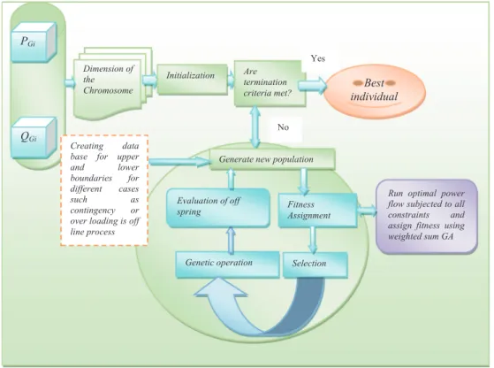
The stopping criterion is either to run this algorithm to reach maximum generation or if the best solution is not improved in successive generations. The architecture of the proposed meth-odology is shown inFig. 1.
5. Procedure
1. By executing OPF in MATPOWER with lower voltage limit as 0.85, increase the load with constant power factor at all buses until a stage where no solution is reached, sub-ject to all other constraints or in the case of base loading with line outage which does not provide solution.
2. Run OPF just ahead of unsolvability for overloading con-dition or in a concon-dition of line outage and calculate NVSI at all buses. Rank load bus in descending order, and select the buses with large value of NVSI as weak buses to per-form load shedding.
3. Generate real random values lie between upper and lower boundaries. Proper selection of these boundaries help to get global optimal solution and it depends on the operator’s knowledge and the cases considered such as overloading or outages. The size of the chromosomes is taken as twice the number of selected load buses for load shedding. Assume suit-able population size and maximum number of generation. 4. Run OPF for all initial generated population individuals
with lower limit voltage is increased to 0.9 pu. Calculate the objective value using Eq.(4).
5. Roulette Wheel Selection (RWS) is used for selection pro-cess. Selected individuals are utilized for genetic operation. Crossover probability and mutation probability is taken as 0.8, 0.1 respectively. Calculate the objective value for off-spring individuals.
6. The individuals are selected for next generation from par-ents and off spring which has minimum objective value.
7. When termination criterion is met, best individual is obtained. The difference between the upper boundary and obtained value of each gene in best individual will give the load shedding at particular load bus.
8. After load shedding run OPF to analyze the performance of the system.
6. Results and discussion
The methodology which is presented in previous sections is illustrated using two different case studies, i.e. IEEE 30 bus system and TNEB 69 practical system in India.
6.1. IEEE 30 bus system
The system comprises 6 generators at buses 1, 2, 5, 8, 11 and 13 and two other buses (#10, 24) with VAR sources and 24 load buses. The network has 41 branches and 4 tap changing transformers in (6–9), (6–10), (4–12) and (28–27) branches. The total base load of the IEEE 30 bus system is 283.4 MW. The proposed algorithm was evaluated using MATLAB and MATPOWER environment on a PC with Pentium core 2 duo processor operating at 2 GHz with 2 GB RAM. In the simulations, the following conditions were implemented. The population size and maximum generation are taken for this system as 50 and 500 respectively.
Loads are modeled as constant power.
The system MVA base is 100.
The power factor of load remains constant when load increases.
This paper presents a particular study for two unsolvable conditions: Case A: heavy loading without contingency, Case B: Base loading with contingency (any one line outage).
6.1.1. Heavy loading without contingency
In this case, the loading at all buses is increased gradually until a stage to reach power flow unsolvability. The IEEE 30 bus system attains unsolvability when the original real and reactive loads are multiplied by multiplication factor (k) 1.6. Proposed weighted sum approach procedure for load shedding, passage of chromosomes into successive generations and termination are shown inFig. 2.
The total real load is increased to 453.44 MW. The power flow analysis converges until the real and reactive loads at all buses are multiplied by 1.59. The real load at this condition is 450.606 MW.
The real load increase at all buses by 2.834 MW (0.01% of base load) will lead to unsolvability and this real load value is considered as total maximum possible load shedding for this case. Five weak buses are selected (5, 30, 10, 24 and 7) for load shedding based on the NVSI values as tabulated inTable 1.
Different loading conditions at selected buses are listed in
Table 2, which would give the knowledge to generate their boundary. The chromosome size is equal to twice the number of selected buses. The chromosome structure is shown in
Fig. 3, first 5 gene values have been generated randomly with in the boundary limits shown in Table 3 and remaining calculated to maintain power factor. For this case, 2–3% of load shedding from maximum limit at all the selected buses is considered lower limit of the boundary.
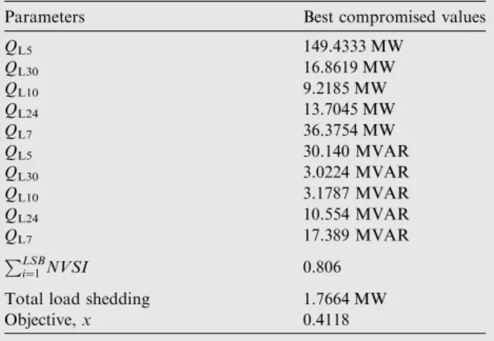
Equal weightages are given for both objective functions withw= 0.5 in this algorithm. In this case, 20 independent
trials are simulated to obtain best compromised solution. The best compromised values of individual and corresponding sum of NVSI at all selected load shedding buses, total load shed-ding and objective for heavy load case are obtained as in
Table 4.
To investigate efficiency of this method, a load shedding of 1.7664 MW is also applied at other buses, and the result shows
that the same load shedding does not restore solvability. The above test concludes that only load shedding at weak buses represents the best options for restoring solvability, and the
Yes Yes No
Generate random chromosome P using real codes within the range of control variables. The size of the chromosomes is 10.
Is it converged?
Increase the load at all bus with constant power factor in steps.
Run OPF using MATPOWER including voltage stability index constraints and reduce minimum voltage constrain to 0.85 pu.
Reduce the load in one step ahead and run OPF. Find NVSI for all lines. Sort it in descending order and select top 5 lines for Load shedding.
Set population size P-max and maximum number of generation G-max.
Run OPF to increase the lower limit voltage is 0.9 and calculate objective value using eqn (4).
Perform selection, crossover and mutation process. Calculate objective value for offspring.
P>P-max
G>G-max P=P+1
P-max individuals are selected for next generation from parent and offspring which has minimum objective value.
G=G+1
The best string is obtained. The difference between the maximum power limit of each selected bus and the obtained value is optimal load shed at that particular bus. Sum of load shedding of all selected bus will give total load shedding .After load shedding run OPF to analyse the system performances.
Figure 2 Flowchart of restoring power flow solvability.
Table 1 Top five weak buses selected for load shedding.
Line Bus NVSI Rank
2–5 5 0.306 1 29–30 30 0.186 2 6–10 10 0.117 3 27–30 30 0.114 2 23–24 24 0.107 4 5–7 7 0.098 5
Table 2 Different loading values for weak buses.
Bus Base loading Heavy loading
Solvable (k= 1.59) Unsolvable (k= 1.6) P(MW) P(MW) P(MW) 5 94.2 149.778 150.72 30 10.6 16.854 16.96 10 5.8 9.222 9.28 24 8.7 13.833 13.92 7 22.8 36.252 36.48
Figure 3 Chromosome structure.
Table 3 Control variable limits for heavy loading condition.
Parameter Limits PL5 (147.7056–150.72) MW PL30 (16.62–16.96) MW PL10 (9.0944–9.28) MW PL24 (13.6416–13.92) MW PL7 (35.7504–36.48) MW
Table 4 Optimized results for heavy loading condition
Parameters Best compromised values
QL5 149.4333 MW QL30 16.8619 MW QL10 9.2185 MW QL24 13.7045 MW QL7 36.3754 MW QL5 30.140 MVAR QL30 3.0224 MVAR QL10 3.1787 MVAR QL24 10.554 MVAR QL7 17.389 MVAR PLSB i¼1NVSI 0.806
Total load shedding 1.7664 MW Objective,x 0.4118
NVSI provides necessary information to correctly indicate the best buses for load shedding.
6.1.2. Heavy loading with contingency
In heavy case loading (k= 1.4), the single line outages 9–11, 9–10,12–13,12–14,10–22,10–21,25–26,28–27 and 27–29 are found to provide no solutions in power flow equations. The line outages 9–11, 12–13, 25–26 and 10–21 cause bus outage and these outages are considered as higher ranking of contin-gency. Other than that, in this case, a particular study for one unsolvable contingency as outage of line 9–10 is presented.
The top seven weak buses listed with their NVSI values in
Table 5are selected for load shedding. The power flow through the line ahead of contingency is 41.22 MW i.e. 12.11% of total demand and this value is considered total maximum possible load shedding for this case.
The chromosome size is equal to 14 and the values are generated within the boundary shown inTable 6. In this case,
Table 9 Control variable limits for TNEB 69 bus system.
Parameter Limits PL56 (220.8–213.9) MW PL51 (137.3–133) MW PL41 (114.3–110.67) MW PL6 (95.04–92.07) MW PL31 (163.2–158.1) MW PL44 (148.8–144.15) MW PL8 (85.44–82.77) MW PL59 (103.68–100.44) MW PL68 (100.8–97.65) MW PL26 (127.68–123.69) MW
Table 10 Optimized results for TNEB 69 bus system.
Parameter Best compromised values
PL56 215.1766 MW PL51 136.9677 MW PL41 112.0173 MW PL6 93.1233 MW PL31 158.7599 MW PL44 146.2108 MW PL8 84.4432 MW PL59 101.7711 MW PL68 98.1552 MW PL26 125.1667 MW QL56 129.1059 MVAR QL51 82.3721 MVAR QL41 67.7751 MVAR QL6 56.4383 MVAR QL31 95.2559 MVAR QL44 87.7264 MVAR QL8 51.2352 MVAR QL59 61.2511 MVAR QL68 58.8931 MVAR QL26 75.2882 MVAR PLSB i¼1NVSI 2.192
Total load shedding 79.2082 MW Objective,x 1.472
Table 5 Top seven weak buses selected for load shedding.
Line Bus NVSI Rank
2–5 5 0.477 1 27–30 30 0.168 2 29–30 30 0.132 2 4–12 12 0.089 3 6–10 10 0.087 4 23–24 24 0.078 5 5–7 7 0.073 6 16–17 17 0.051 7
Table 6 Control variable limits for heavy loading with contingency condition. Parameter Limits PL5 (92.6928–96.084) MW PL30 (10.4304–10.812) MW PL12 (11.0208–11.424) MW PL10 (5.7072–5.916) MW PL24 (8.5608–8.874) MW PL7 (23.256–24.4352) MW PL17 (8.856–9.1811) MW
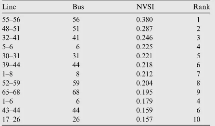
Table 8 Top ten weak buses selected for load shedding.
Line Bus NVSI Rank
55–56 56 0.380 1 48–51 51 0.287 2 32–41 41 0.246 3 5–6 6 0.225 4 30–31 31 0.221 5 39–44 44 0.218 6 1–8 8 0.212 7 52–59 59 0.204 8 65–68 68 0.195 9 1–6 6 0.179 4 43–44 44 0.159 6 17–26 26 0.157 10
Table 7 Optimized results for heavy loading with contingency.
Parameters Best compromised values PL5 94.952 MW PL30 10.5513 MW PL12 11.2946 MW PL10 5.7715 MW PL24 8.6257 MW PL7 23.9541 MW PL17 8.9132 MW QL5 19.15168 MVAR QL30 1.89123 MVAR QL10 7.5633 MVAR QL24 1.9901 MVAR QL7 11.4517 MVAR PLSB i¼1NVSI 0.591
Total load shedding 30.6979 MW Objective,x 0.310
15% of load shedding at all the selected buses is taken as lower boundary limit and 18% of load shedding is treated as higher boundary limit which cover the maximum possible load shedding.
Table 7shows the best compromised solution with total load shedding of 30.6979 MW which is less than the 41.22 MW. As it can be seen, a load shedding of 30.6979 MW distributed on these seven buses is sufficient to bring the system to a solvable area and represents only 9% of the total system demand.
6.2. TNEB 69 bus system
A practical system TNEB 69 in India is considered as Test sys-tem II. This has 13 generator buses, 56 load buses and 99 inter-connected lines [20]. The Tap changing transformers are provided at 11 branches in this practical system. The popula-tion size and maximum generapopula-tion are taken for this system as 50 and 500 respectively.
The single line outages 47–48, 15–28, 28–29, 41–48, 60–64 and 65–68 in base case loading can lead the system to unsolv-able region. The unsolvunsolv-able contingency 41–48 is only consid-ered for this case. The top ten weak buses with their NVSI values are shown inTable 8. The real power flow in this line is 245.328 MW and this is maximum possible load shedding in this case.
In this case, 4% of load shedding at all the selected buses is taken as lower boundary limit and 7% of load shedding is trea-ted as higher boundary limit which cover the maximum possi-ble load shedding. The size of the chromosome is 20 and the limits of generation are given inTable 9.
The compromised solution for this case is shown in
Table 10. The load shedding of 79.2082 MW is enough to retune the system to become solvable region. The results show that each contingency leads to a different scenario, the most favorable of these parameters depend on the system and their operating conditions. Our experience indicates that choosing the control variable limits and proper number of buses selected for load shedding based on the working experience in off-line will give good results for on-line also.
7. Conclusion
This work has proposed an optimization algorithm to deter-mine the optimal location and amount of load shed to retain solvability margin of power flow solution. Load shedding is
the ultimate remedy to save the system from complete black out. To avoid voltage collapse, when the system is in non-cor-rectable emergency, load shedding is the last resort. The weak buses which are identified using NVSI have been proved as optimal location of load shed and also the weighted sum genetic algorithm to ensure the less number of locations and minimum amount of load shed in selected locations. The test results on IEEE 30 bus system and TNEB 69 bus practical sys-tem in India for both the cases of heavy loading and contin-gency condition show that the load shedding method can be applied to restore power flow solvability in a computationally efficient manner.
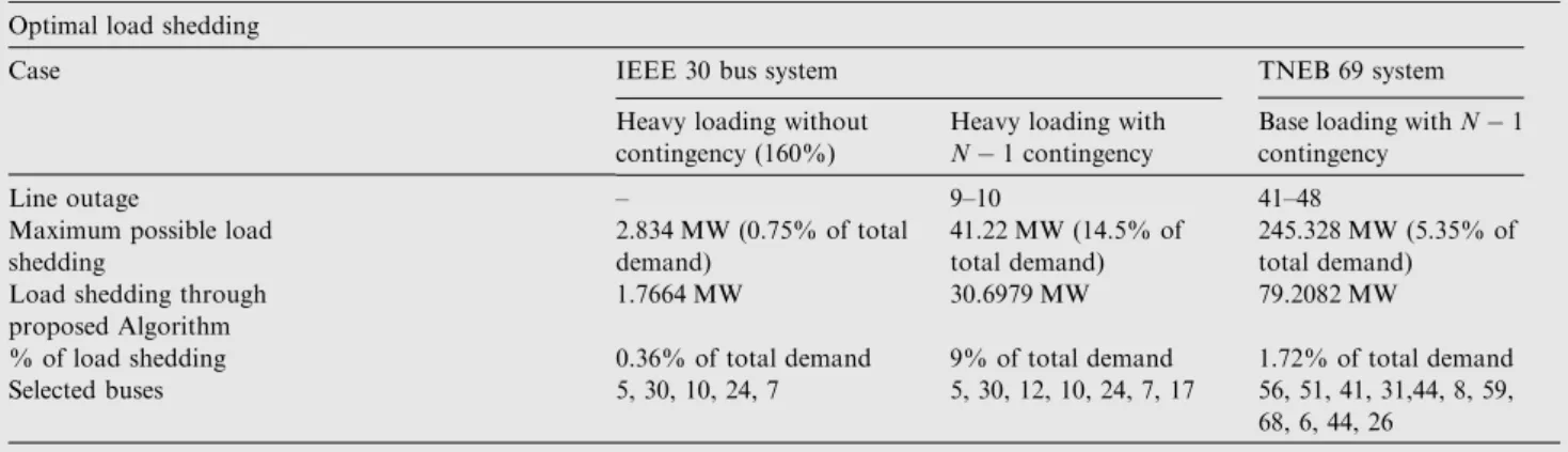
FromTable 11, the load shedding is possible through this method with less % of load shed in less number of selected buses. Although the solution cannot be guaranteed to obtain the global optimum results of the problem, it works better for local optimum. This method provides optimal recommen-dation of the department and independent variable of power system to return from unsolvable region to feasible region. Since the algorithm is based upon a power flow solution, it should be quite easy to integrate with existing security enhancement applications.
References
[1]M.A. Mostafa, M.E. El-Hawary, G.A.N. Mbamalu, M.M. Mansour, KM. El-Nagar, A.N. El-Arabaty, Steady-state load shedding schemes: a performance comparison, Electr. Pow. Syst. Res. 38 (1996) 105–112.
[2]M.Z. El-Sadek, G.A. Mahmoud, M.M. Dessouky, W.I. Rashed, Optimum load shedding for avoiding steady-state voltage instability, Electr. Pow. Syst. Res. 50 (1999) 119–123.
[3]D. Hazarika, A.K. Sinha, Method for optimal load shedding in case of generation deficiency in a power system, Electr. Pow. Energy Syst. 20 (1998) 411–420.
[4]Deb Chattopadhyay, Bhujanga B. Chakrabarti, A preventive/ corrective model for voltage stability incorporating dynamic load-shedding, Electr. Pow. Energy Syst. 25 (2003) 363–376. [5]F.M. Echavarren, E. Lobato, L. Rouco, A corrective load
shedding scheme to mitigate voltage collapse, Electr. Pow. Energy Syst. 28 (2006) 58–64.
[6]T. Amraee, A.M. Ranjbar, B. Mozafari, N. Sadati, An enhanced under-voltage loadshedding scheme to provide voltage stability, Electr. Pow. Syst. Res. 77 (2007) 1038–1046.
[7]L.D. Arya, Pushpendra Singh, L.S. Titare, Optimum load shedding based on sensitivity to enhance static voltage stability using DE, Swarm Evol. Comput. 6 (2012) 5–38.
Table 11 Experimental results for proposed method.
Optimal load shedding
Case IEEE 30 bus system TNEB 69 system Heavy loading without
contingency (160%)
Heavy loading with
N1 contingency
Base loading withN1 contingency
Line outage – 9–10 41–48
Maximum possible load shedding 2.834 MW (0.75% of total demand) 41.22 MW (14.5% of total demand) 245.328 MW (5.35% of total demand) Load shedding through
proposed Algorithm
1.7664 MW 30.6979 MW 79.2082 MW
% of load shedding 0.36% of total demand 9% of total demand 1.72% of total demand Selected buses 5, 30, 10, 24, 7 5, 30, 12, 10, 24, 7, 17 56, 51, 41, 31,44, 8, 59,
[8]L.D. Arya, Pushpendra Singh, L.S. Titare, Differential evolution applied for anticipatory load shedding with voltage stability considerations, Electr. Pow. Energy Syst. 42 (2012) 644–652.
[9]J.A. Laghari, H. Mokhlis, A.H.A. Bakar, Hasmaini Mohamad, Application of computational intelligence techniques for load shedding in power systems: a review, Energy Convers. Manage. 75 (2013) 130–140.
[10]T.J. Overbye, A power flow measure for unsolvable cases, IEEE Trans. Power Syst. 9 (1994) 1359–1365.
[11]Vaibhav Donde, Vanessa Lo´pez, Bernard Lesieutre, Ali Pinar, Chao Yang, Juan Meza, Severe multiple contingency screening in electric power systems, IEEE Trans. Power Syst. 23 (2008) 406–417. [12]Xu Fu, Xifan Wanga, Determination of load shedding to provide
voltage stability, Electr. Pow. Energy Syst. 33 (2011) 515–521. [13]Mitsuo Gen, Lin Lin, Jung-Bok Jo, Evolutionary network design
by multiobjective hybrid genetic algorithm, Intelligent and Evolutionary Systems, vol. 187, Springer, 2009, pp. 105–121. [14] M. Sanaye-Pasand, M. Davarpanah, A new adaptive
multidimensional load shedding scheme using genetic algorithm, in: IEEE Canadian Conference on Electrical and Computer Eng, Saskatchewan Canada, May 1–4, 2005, pp. 1974–1977.
[15] B.F. Rad, M. Abedi, An optimal load-shedding scheme during contingency situations using meta-heuristics algorithms with application of AHP method, in: IEEE Optimization of Electrical and Electronics Equipment, Brasov, Romania, May 22–24, 2008, pp. 167–73.
[16] C. Chao-Rong, T. Wen-Ta, C. Hua-Yi, L. Ching-Ying, C. Chun-Ju, L. Hong-Wei, Optimal load shedding planning with genetic algorithm, in: IEEE Industrial Application Society annual meeting, Orlando, Oct. 9–13, 2011, pp. 1–6.
[17]Luan WP, Irving MR, Daniel JS, Genetic algorithm for supply restoration and optimal load shedding in power system distribution networks, IET Gener. Trans. Distrib. 149 (2002) 45–51.
[18]R. Kanimozhi, K. Selvi, A novel line stability index for voltage stability analysis and contingency ranking in power system using fuzzy based load flow, J. Electr. Eng. Technol. 8 (2013) 694–703. [19]Mitsuo Gen, Runwei Cheng, Lin Lin, Network, Models and Optimization Multi objective Genetic Algorithm Approach, Springer, 2008.
[20] Tamil Nadu Electricity Board Statistics at a Glance 2009–2010, Planning Wing of Tamil Nadu Electricity Board, Chennai, India.