Selection of our books indexed in the Book Citation Index in Web of Science™ Core Collection (BKCI)
Interested in publishing with us?
Contact [email protected]
Numbers displayed above are based on latest data collected. For more information visit www.intechopen.com Open access books available
Countries delivered to Contributors from top 500 universities
International authors and editors
Our authors are among the
most cited scientists
Downloads
We are IntechOpen,
the world’s leading publisher of
Open Access books
Built by scientists, for scientists
12.2%
122,000
135M
TOP 1%
154
Using Opposition-based Learning with Particle
Swarm Optimization and Barebones Differential
Evolution
Mahamed G.H. Omran
Gulf University for Science and Technology
Kuwait
1. Introduction
Particle swarm optimization (PSO) (Kennedy & Eberhart, 1995) and differential evolution (DE) (Storn & Price, 1995) are two stochastic, population-based optimization methods, which have been applied successfully to a wide range of problems as summarized in Engelbrecht (2005) and Price et al. (2005).
A number of variations of both PSO and DE have been developed in the past decade to improve the performance of these algorithms (Engelbrecht, 2005; Price et al. 2005). One class of variations includes hybrids between PSO and DE, where the advantages of the two approaches are combined. The barebones DE (BBDE) is a PSO-DE hybrid algorithm proposed by Omran et al. (2007) which combines concepts from the barebones PSO (Kennedy 2003) and the recombination operator of DE. The resulting algorithm eliminates the control parameters of PSO and replaces the static DE control parameters with dynamically changing parameters to produce an almost parameter-free, self-adaptive, optimization algorithm.
Recently, opposition-based learning (OBL) was proposed by Tizhoosh (2005) and was successfully applied to several problems (Rahnamayan et al., 2008). The basic concept of OBL is the consideration of an estimate and its corresponding opposite estimate simultaneously to approximate the current candidate solution. Opposite numbers were used by Rahnamayan et al. (2008) to enhance the performance of Differential Evolution. In addition, Han and He (2007) and Wang et al. (2007) used OBL to improve the performance of PSO. However, in both cases, several parameters were added to the PSO that are difficult to tune. Wang et al. (2007) used OBL during swarm initialization and in each iteration with a user-specified probability. In addition, Cauchy mutation is applied to the best particle to avoid being trapping in local optima. Similarly, Han and He (2007) used OBL in the initialization phase and also during each iteration. However, a constriction factor is used to enhance the convergence speed.
In this chapter, OBL is used to improve the performance of PSO and BBDE without adding any extra parameter. The performance of the proposed methods is investigated when applied to several benchmark functions. The experiments conducted show that OBL improves the performance of both PSO and BBDE.
The remainder of the chapter is organized as follows: PSO is summarized in Section 2. DE is presented in Section 3. Section 4 provides an overview of BBDE. OBL is briefly reviewed in
Section 5. The proposed methods are presented in Section 6. Section 7 presents and discusses the results of the experiments. Finally, Section 8 concludes the chaper.
2. Particle Swarm Optimization
Particle swarm optimization (PSO) is a stochastic, population-based optimization algorithm modeled after the simulation of social behavior of bird flocks. In a PSO system, a swarm of individuals (called particles) fly through the search space. Each particle represents a candidate solution to the optimization problem. The position of a particle is influenced by the best position visited by itself (i.e. its own experience) and the position of the best particle in its neighborhood (i.e. the experience of neighboring particles). Particle position, xi, are adjusted using
)
1
(
)
(
)
1
(
t
+
=
it
+
it
+
ix
v
x
(1)where the velocity component, vi, represents the step size. For the basic PSO,
v
i,j(
t
+
1)
=
wv
i,j(
t
)
+
c
1r
1,j(
t
)(
y
i,j(
t
)
−
x
i,j(
t
))
+
c
2r
2,j(
t
)(
y
ˆ
j(
t
)
−
x
i,j(
t
))
(2) where w is the inertia weight (Shi & Eberhart, 1998), c1 and c2 are the accelerationcoefficients,
j
r1, , r2,j ~U(0,1), yi is the personal best position of particle i, and ˆyi is the
neighborhood best position of particle i.
The neighborhood best position
ˆ
y
i, of particle i depends on the neighborhood topology used (Kennedy, 1999; Kenedy & Mendes, 2002). If a fully-connected topology is used, theni
ˆ
y
refers to the best position found by the entire swarm. That is,}
{
0 1{
0 1 s}
ˆ
i( ), ( ),..., ( )
s( ( )), ( ( )),..., ( ( ))
y (t)
∈
y t y t
y t
=
min f y t
f y t
f y t
(3) where s is the swarm size.The resulting algorithm is referred to as the global best (gbest) PSO. A pseudo-code for PSO is shown in Alg. 1.
for each particle i∈ 1,...,s do Randomly initialize xi
Set vi to zero
Set yi = xi
endfor Repeat
for each particle i∈ 1,...,s do
Evaluate the fitness of particle i, f(xi)
Update yi
Updateˆy using equation (3) for each dimension j∈ 1,...,Nddo
Apply velocity update using equation (2) endloop
Apply position update using equation (1) endloop
Until some convergence criteria is satisfied Algorithm 1. General pseudo-code for PSO
Van den Bergh and Engelbrecht (2006) and Clerc and Kennedy (2002) proved that each particle converges to a weighted average of its personal best and neighborhood best position, that is,
2 1 j i, 2 j i, 1 j i, t
c
c
y
ˆ
c
y
c
t
x
+
+
=
+∞ →(
)
lim
This theoretically derived behavior provides support for the barebones PSO developed by Kennedy (2003). It replaces Eqs. 1 and 2 with
⎟⎟
⎠
⎞
⎜⎜
⎝
⎛
+
=
+
(
)
-
(
)
2
)
(
)
(
)
1
(
t
N
y
t
y
ˆ
t
,
y
t
ˆ
y
t
x
i,j i,j j i,j jParticle positions are therefore randomly selected from a Gaussian distribution with the mean given as the weighted average of the personal best and global best positions, i.e. the swarm attractor. Note that exploration is facilitated via the deviation,
y
i, j(
t
)-
ˆy
j(
t
)
, which approaches zero as t increases. In the limit, all particles will converge on the attractor point. Kennedy (2003) also proposed an alternative version of the barebones PSO where Eqs. 1 and 2 are replaced with⎪
⎩
⎪
⎨
⎧
>
⎟⎟
⎠
⎞
⎜⎜
⎝
⎛
+
=
+
otherwise
)
(
0.5
(0,1)
if
)
(
-)
(
2
)
(
)
(
)
1
(
t
y
U
t
y
ˆ
t
y
,
t
y
ˆ
t
y
N
t
x
j i, j j i, j j i, j i,Based on the above equation, there is a 50% chance that the j-th dimension of the particle dimension changes to the corresponding personal best position. This version of PSO biases towards exploiting personal best positions.
3. Differential Evolution
Differential evolution (DE) is an evolutionary algorithm proposed by Storn and Price (1995). While DE shares similarities with other evolutionary algorithms (EA), it differs significantly in the sense that distance and direction information from the current population is used to guide the search process. DE uses the differences between randomly selected vectors (individuals) as the source of random variations for a third vector (individual), referred to as the target vector. Trial solutions are generated by adding weighted difference vectors to the target vector. This process is referred to as the mutation operator where the target vector is mutated. A recombination, or crossover step is then applied to produce an offspring which is only accepted if it improves on the fitness of the parent individual.
The basic DE algorithm is described in more detail below with reference to the three evolution operators: mutation, crossover, and selection.
Mutation: For each parent, xi(t), of generation t, a trial vector, vi(t), is created by mutating a target vector. The target vector,
(
)
3
t
iindividuals ( ) 1 t i x , and
(
)
2t
ix
are randomly selected with i1 ≠ i2 ≠ i3 ≠ i, and the difference vector, 1 ix
- 2 ix
, is calculated. The trial vector is then calculated as))
(
-)
(
(
)
(
)
(
2 1 3t
F
t
t
t
i i i ix
x
x
v
=
+
(4)where the last term represents the mutation step size. In the above, F is a scale factor used to control the amplification of the differential variation. Note that F∈ (0, ∞).
Crossover: DE follows a discrete recombination approach where elements from the parent vector,
x
i(
t
)
, are combined with elements from the trial vector,v
i(
t
)
, to produce the offspring,μ
i(
t
)
. Using the binomial crossover,µ
ij(
t
)
=
v
ij(
t
)
if
U
(
0
,
1
)
<P
ror
j
=
r
x
ij(
t
)
otherwise
⎧
⎨
⎩
where j = 1, ..., Nd refers to a specific dimension, Nd is the number of genes (parameters) of a
single chromosome, and r ~ U(1,…, Nd). In the above, pr is the probability of reproduction
(with pr∈ [0, 1]).
Thus, each offspring is a stochastic linear combination of three randomly chosen individuals when U(0, 1) < pr; otherwise the offspring inherits directly from the parent. Even when pr =
0, at least one of the parameters of the offspring will differ from the parent (forced by the condition j = r).
Selection: DE evolution implements a very simple selection procedure. The generated offspring,
μ
i(
t
)
, replaces the parent,x
i(
t
)
, only if the fitness of the offspring is better thanthat of the parent.
4. Barebones Differential Evolution
Both PSO and DE have their strengths and weaknesses. PSO has the advantage that formal proofs exist to show that particles will converge to a single attractor. The barebones PSO utilizes this information by sampling candidate solutions, normally distributed around the formally derived attractor point. Additionally, the barebones PSO has no parameters to be tuned. On the other hand, DE has the advantage of not being biased towards any prior defined distribution for sampling mutational step sizes and its selection operator follows a hill-climbing process. Mutational step sizes are determined as differences between individuals in the current population. One of the problems which both PSO and DE share is that control parameters need to be optimized for each new problem.
The barebones DE combines the strengths of both the barebones PSO and DE to form a new, efficient hybrid optimization algorithm. For the barebones DE, position updates are done as follows:
⎩
⎨
⎧
+
×
>
=
otherwise
)
(
1)
(0,
if
))
(
-)
(
(
)
(
)
(
2 1 2t
y
p
U
t
x
t
x
r
t
p
t
x
j , i r j , i j , i j , j i, j i, 3 (5)where
)
(
))
(
1
(
)
(
)
(
)
(
t
r
1t
y
t
r
1t
ˆ
y
t
p
i,j=
,j i,j+
−
,j i,j (6)with i1, i2, i3~ U(1,…,s), i1 ≠ i2 ≠ i,
r
1,j,r
2,j~
U
(0,1)
and pr is the probability ofrecombination.
Referring to Eq. 6,
p
i(
t
)
represents the particle attractor as a stochastic weighted average of personal best and global best positions, borrowing from the barebones PSO (Kennedy 2003). Referring to Eq. 5, the mutation operator of DE is used to explore around the current attractor,p
i(
t
)
, by adding a difference vector to the attractor. Crossover is done with arandomly selected personal best,
3
i
y
, as these personal bests represent a memory of best solutions found by individuals since the start of the search process. Also note that the scale factor is a random variable. Using the position update in Eq. 6, for a proportion of (1- pr) ofthe updates, information from a randomly selected personal best,
3
i
y
, is used (facilitating exploitation), while for a proportion of pr of the updates step sizes are mutations of theattractor point, pi (facilitating exploration). Mutation step sizes are based on the difference vector between randomly selected particles,
1
i
x
and2
i
x
. Using the above, the BBDE achieves a good balance between exploration and exploitation. It should also be noted that the exploitation of personal best positions does not focus on a specific position. The personal best position,3
i
y
, is randomly selected for each application of the position update.5. Opposition-based Learning
Opposition-based learning (OBL) was first proposed by Tizhoosh (2005) and was successfully applied to several problems (Rahnamayan et al., 2008). Opposite numbers are defined as follows:
Let x∈[a,b], then the opposite number x’ is defined as
x
'=
a
+
b
−
x
The above definition can be extended to higher dimensions as follows:
Let
P x x
(
1,
2,
,
x
n)
be an n-dimensional vector, where xi ∈[ai,bi] and i=1, 2, …, n. Theopposite vector of P is defined by
P x x
′ ′ ′
(
1,
2,
,
x
n′
)
wherex
'i=
a
i+
b
i−
x
i6. Proposed Methods
In this chapter, OBL is used to enhance the performance of PSO and BBDE without adding any extra parameter. Two variants are proposed as follows:
6.1 Improved PSO (iPSO)
An improved version of PSO is proposed such that in each iteration the particle with the lowest fitness, xb, is replaced by its opposite (the anti-particle) as follows,
xb,j = LBj + UBj – xb,j
where xb,j∈[LBj, UBj], j=1,2,…,Nd and Nd is the dimension of the problem.
The velocity and personal experience of the anti-particle are reset. The global best solution is also updated. A pseudo-code for iPSO is shown in Alg. 2.
The rationale behind this approach is the basic idea of opposition-based learning: if we begin with a random guess, which is very far away from the existing solution, let say in worst case it is in the opposite location, then we should look in the opposite direction. In our case, the guess that is “very far away from the existing solution” is the particle with the lowest fitness.
The main difference between iPSO on one side and the approaches proposed by Han and He (2007) and Wang et al. (2007) on the other side, is that we did not introduce any extra parameter to the original PSO. In addition, iPSO uses only OBL to enhance the performance of PSO while (Han & He, 2007; Wang et al. 2007) use OBL combined with other techniques (e.g. Cauchy mutation).
for each particle i∈ 1,...,s do for each dimension j∈ 1,...,Nd do
xi,j = LBj+ rj× (UBj – LBj)
endloop endfor
for each particle i∈ 1,...,s do Set vi to zero
Set yi = xi
endfor Repeat
for each particle i∈ 1,...,s do
Evaluate the fitness of particle i, f(xi)
Update yi
Updateˆy using equation (3) for each dimension j∈ 1,...,Nd do
Apply velocity update using Eq. (2) endloop
Apply position update using equation (1) endloop
Let xb be the particle with the lowest fitness
for each dimension j∈ 1,...,Nd do
xb,j = LBj + UBj – xb,j endloop vb = 0 yb = xb if f(xb) < f(ˆy) y ˆ = xb endif
Until some convergence criteria is satisfied
6.2 Improved BBDE (iBBDE)
Similar to iPSO, BBDE is modified such that in each iteration the particle with the lowest fitness, xb, is replaced by its opposite. The personal experience of the anti-particle is also
reset. The global best solution is updated.
7. Experimental Results
This section compares the performance of the proposed methods with that of gbest PSO and BBDE discussed in Section 2 and 4, respectively. For the PSO algorithms, w = 0.72 and c1 = c2 = 1.49. These values have been shown to provide very good results (van den Berg, 2002). In addition s = 50 for all methods. All functions were implemented in 30 dimensions.
The following functions have been used to compare the performance of the different approaches. These benchmark functions provide a balance of unimodal, multimodal, separable and non-separable functions.
For each of these functions, the goal is to find the global minimizer, formally defined as Given f: ℜNd åℜ
find
x
∗∈
ℜ
Nd such thatf
(
x
∗)
≤
f
(
x
),
∀
x
∈
ℜ
NdThe following functions were used: A. Sphere function, defined as
∑
==
d N i ix
f
1 2)
(
x
where
x
∗=
0
andf
(
x
∗)
=
0
for−
100
≤
≤
100
i
x
.B. Rosenbrock function, defined as
f
(
x
)
=
(
100
(
x
i−
x
i2−1)
2+
(
x
i−1−
1
)
2)
i=1 Nd−1
∑
where
x
∗=
(
1
,
1
,
…
,
1
)
andf
(
x
∗)
=
0
for−
2
≤
x
i≤
2
. C. Rotated hyper-ellipsoid function, defined as∑ ∑
= =⎟⎟
⎠
⎞
⎜⎜
⎝
⎛
=
d N i i j jx
f
1 2 1)
(
x
where
x
∗=
0
andf
(
x
∗)
=
0
for−
100
≤
≤
100
ix
.(
)
∑
=+
−
=
d N i i ix
x
f
1 210
)
π
2
cos(
10
)
(
x
where
x
∗=
0
andf
(
x
∗)
=
0
for5
.
12
x
5
.
12
i≤
≤
−
.E. Ackley's function, defined as
f
(
x
)
= −
20exp -0.2
1
30
x
i 2 i=1 Nd∑
⎛
⎝
⎜
⎞
⎠
⎟
−
exp
1
30
i=1cos(2
πx
i)
Nd∑
⎛
⎝
⎜
⎞
⎠
⎟
+
20
+
e
where
x
∗=
0
andf
(
x
∗)
=
0
for−
32
≤
≤
32
i
x
. F. Griewank function, defined as1
cos
4000
1
)
(
1 1 2+
⎟
⎠
⎞
⎜
⎝
⎛
−
=
∑
∏
= = d d N i N i i ii
x
x
f
x
where
x
∗=
0
andf
(
x
∗)
=
0
for−
600
≤
≤
600
ix
.G. Salomon function, defined as
f
(
x
)
= −
cos 2
π
x
i2 i=1 Nd∑
⎛
⎝
⎜
⎞
⎠
⎟
+
0
.
1
x
i 2 i=1 Nd∑
+
1
where
x
∗=
0
andf
(
x
∗)
=
0
for−
100
≤
≤
100
ix
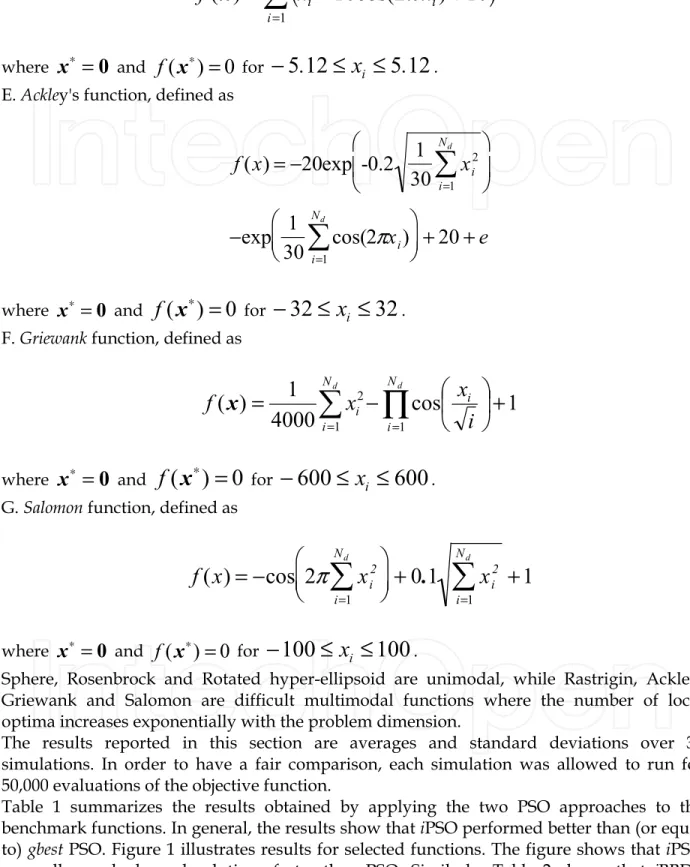
.Sphere, Rosenbrock and Rotated hyper-ellipsoid are unimodal, while Rastrigin, Ackley, Griewank and Salomon are difficult multimodal functions where the number of local optima increases exponentially with the problem dimension.
The results reported in this section are averages and standard deviations over 30 simulations. In order to have a fair comparison, each simulation was allowed to run for 50,000 evaluations of the objective function.
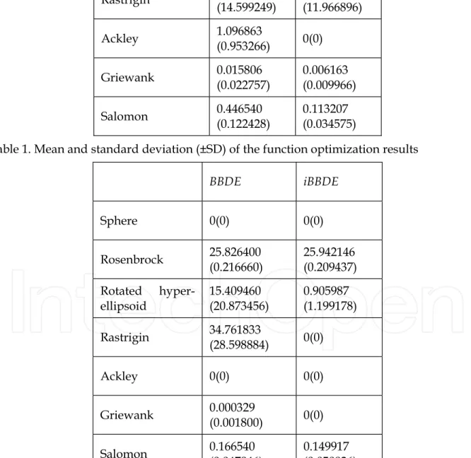
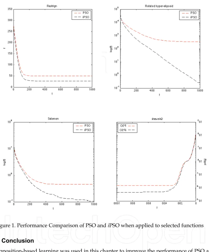
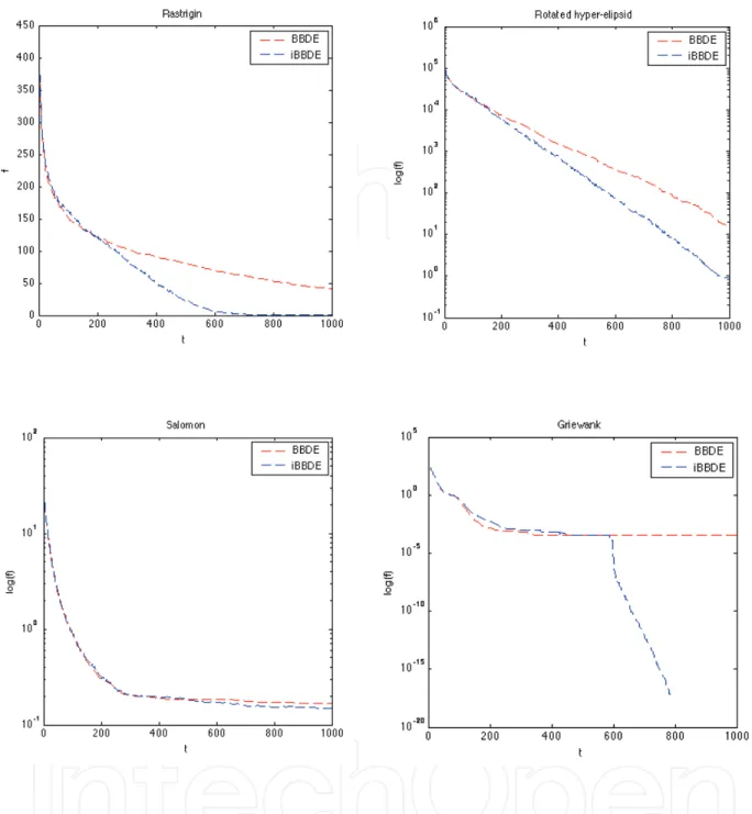
Table 1 summarizes the results obtained by applying the two PSO approaches to the benchmark functions. In general, the results show that iPSO performed better than (or equal to) gbest PSO. Figure 1 illustrates results for selected functions. The figure shows that iPSO generally reached good solutions faster than PSO. Similarly, Table 2 shows that iBBDE generally outperformed BBDE. Figure 2 illustrates results for selected functions. Thus, Tables 1 and 2 suggest that using the simple idea of replacing the worst particle is the main reason for improving the performance of PSO and BBDE. In additon, we can conclude that
opposition-based learning improved the performance of both PSO and BBDE without requiring any extra parameter.
PSO iPSO Sphere 0(0) 0(0) Rosenbrock 22.191441 (1.741527) 20.645323 (0.426212) Rotated hyper-ellipsoid 2.021006 (1.675313) 0.355572 (0.890755) Rastrigin 48.487584 (14.599249) 27.460845 (11.966896) Ackley 1.096863 (0.953266) 0(0) Griewank 0.015806 (0.022757) 0.006163 (0.009966) Salomon 0.446540 (0.122428) 0.113207 (0.034575)
Table 1. Mean and standard deviation (±SD) of the function optimization results
BBDE iBBDE Sphere 0(0) 0(0) Rosenbrock 25.826400 (0.216660) 25.942146 (0.209437) Rotated hyper-ellipsoid 15.409460 (20.873456) 0.905987 (1.199178) Rastrigin 34.761833 (28.598884) 0(0) Ackley 0(0) 0(0) Griewank 0.000329 (0.001800) 0(0) Salomon 0.166540 (0.047946) 0.149917 (0.050826)
Figure 1. Performance Comparison of PSO and iPSO when applied to selected functions
7. Conclusion
Opposition-based learning was used in this chapter to improve the performance of PSO and BBDE. Two opposition-based variants were proposed (namely, iPSO and iBBDE). The iPSO and iBBDE algorithms replace the least-fit particle with its anti-particle. The results show that, in general, iPSO and iBBDE outperformed PSO and BBDE, respectively. In addition, the results show that using OBL enhances the performance of PSO and BBDE without requiring additional parameters. The ideas introduced in this chapter could also be used with any PSO/BBDE variant.
Future research will investigate the effect of noise on the performance of the proposed approaches. Furthermore, a scalability study will be conducted. Finally, applying the proposed approaches to real-world problem will be investigated.
Figure 2. Performance Comparison of BBDE and iBBDE when applied to selected functions
8. References
Clerc, M. & Kennedy, J. (2002). The Particle Swarm-Explosion, Stability, and Convergence in a Multidimensional Complex Space. IEEE Transactions on Evolutionary Computation, Vol. 6, No. 1, pp. 58-73.
Engelbrecht, A. (2005). Fundamentals of Computational Swarm Intelligence, Wiley & Sons. Han, L. & He, X. (2007). A novel Opposition-based Particle Swarm Optimization for Noisy
Problems. Proceedings of the Third International Conference on Natural Computation, IEEE Press, Vol. 3, pp. 624 – 629.
Kennedy, J. (1999). Small Worlds and Mega-Minds: Effects of Neighborhood Topology on Particle Swarm Performance. Proceedings of the IEEE Congress on Evolutionary Computation, Vol. 3, pp. 1931-1938.
Kennedy, J. (2003). Bare Bones Particle Swarms. Proceedings of the IEEE Swarm Intelligence Symposium, pp. 80-87.
Kennedy, J. & Eberhart, R. (1995). Particle Swarm Optimization. Proceedings of the IEEE International Joint Conference on Neural Networks, pp. 1942-1948.
Kennedy, J. & Mendes, R. (2002). Population Structure and Particle Performance. Proceedings of the IEEE Congress on Evolutionary Computation, pp. 1671-1676, IEEE Press.
Omran, M., Engelbrecht, A. & Salman, A. (2007). Differential evolution based on particle swarm optimization. Proceedings of the IEEE Swarm Intelligence Symposium, pp. 112-119.
Price, K.; Storn, R. & Lampinen, J. (2005). Differential Evolution: A Practical Approach to Global Optimization, Springer.
Rahnamayan, S.; Tizhoosh, H. & Salama, M. (2008). Opposite-based Differential Evolution.
IEEE Trans. On Evolutionary Computation, Vol. 12, No. 1, pp. 107-125.
Shi, Y. & Eberhart, R. (1998). A Modified Particle Swarm Optimizer. Proceedings of the IEEE Congress on Evolutionary Computation, pp. 69-73.
Storn, R. & Price, K. (1995). Differential evolution - A Simple and efficient adaptive scheme for global optimization over continuous spaces. Technical Report TR-95-012, International Computer Science Institute.
Tizhoosh, H. (2005). Opposition-based Learning: A New Scheme for Machine Intelligence.
Proceedings Int. Conf. Comput. Intell. Modeling Control and Autom, Vol. I, pp. 695-701. van den Bergh, F. (2002). An Analysis of Particle Swarm Optimizers. PhD thesis, Department
of Computer Science, University of Pretoria, Pretoria, South Africa, 2002.
van den Bergh, F. & Engelbrecht, A. (2006). A Study of Particle Swarm Optimization Particle Trajectories. Information Sciences, Vol. 176, No. 8, pp. 937-971.
Wang, H.; Liu, Y.; Zeng, S.; Li, H. & Li, C. (2007). Opposition-based Particle Swarm Algorithm with Cauchy Mutation. Proceedings of the IEEE Congress on Evolutionary Computation, pp. 4750-4756.
ISBN 978-953-7619-48-0 Hard cover, 476 pages
Publisher InTech
Published online 01, January, 2009
Published in print edition January, 2009
InTech Europe
University Campus STeP Ri Slavka Krautzeka 83/A 51000 Rijeka, Croatia Phone: +385 (51) 770 447 Fax: +385 (51) 686 166 www.intechopen.com
InTech China
Unit 405, Office Block, Hotel Equatorial Shanghai No.65, Yan An Road (West), Shanghai, 200040, China
Phone: +86-21-62489820 Fax: +86-21-62489821
Particle swarm optimization (PSO) is a population based stochastic optimization technique influenced by the social behavior of bird flocking or fish schooling.PSO shares many similarities with evolutionary computation techniques such as Genetic Algorithms (GA). The system is initialized with a population of random solutions and searches for optima by updating generations. However, unlike GA, PSO has no evolution operators such as crossover and mutation. In PSO, the potential solutions, called particles, fly through the problem space by following the current optimum particles. This book represents the contributions of the top researchers in this field and will serve as a valuable tool for professionals in this interdisciplinary field.
How to reference
In order to correctly reference this scholarly work, feel free to copy and paste the following:
Mahamed G.H. Omran (2009). Using Opposition-based Learning with Particle Swarm Optimization and Barebones Differential Evolution, Particle Swarm Optimization, Aleksandar Lazinica (Ed.), ISBN: 978-953-7619-48-0, InTech, Available from:
http://www.intechopen.com/books/particle_swarm_optimization/using_opposition-based_learning_with_particle_swarm_optimization_and_barebones_differential_evolutio