Development of a wake model for wind farms based on an open source CFD solver. Strategies on parabolization and turbulence modeling

Development of a wake model for wind farms

based on an open source CFD solver. Strategies on

parabolization and turbulence modeling

PhD Thesis

Daniel Cabezón Martínez

Departamento de Ingeniería Energética y Fluidomecánica, Escuela Técnica Superior de Ingenieros Industriales, Universidad Politécnica de Madrid (UPM), Madrid, Spain

i

Abstract

Wake effect represents one of the most important aspects to be analyzed at the engineering phase of every wind farm since it supposes an important power deficit and an increase of turbulence levels with the consequent decrease of the lifetime. It depends on the wind farm design, wind turbine type and the atmospheric conditions prevailing at the site.

Traditionally industry has used analytical models, quick and robust, which allow carry out at the preliminary stages wind farm engineering in a flexible way. However, new models based on Computational Fluid Dynamics (CFD) are needed. These models must increase the accuracy of the output variables avoiding at the same time an increase in the computational time.

Among them, the elliptic models based on the actuator disk technique have reached an extended use during the last years. These models present three important problems in case of being used by default for the solution of large wind farms: the estimation of the reference wind speed upstream of each rotor disk, turbulence modeling and computational time.

In order to minimize the consequence of these problems, this PhD Thesis proposes solutions implemented under the open source CFD solver OpenFOAM and adapted for each type of site: a correction on the reference wind speed for the general elliptic models, the semi-parabollic model for large offshore wind farms and the hybrid model for wind farms in complex terrain.

All the models are validated in terms of power ratios by means of experimental data derived from real operating wind farms.

ii

Acknowledgements

First of all, I would like to thank sincerely to Professor Antonio Crespo and Emilio Migoya for their kind support and their nice advices along the last years during my regular visits to the laboratory. It has been a tremendous pleasure to work together and I hope we can continue doing so during the next years on the countless areas in wind energy that still remain open.

Also thanks indeed to Kurt Hansen (DTU, Denmark) and Gerard Schepers (ECN, The Netherlands), two of my closest colleagues at the UPWIND project, for their unforgettable support during those 5 years and for sharing their experience to get accurate data bases to validate all the wake models that we analyzed. This project represented one my most satisfying and delighting personal and professional experiences of my late career.

I’d also like to show my gratitude to my big friend Jonathon Sumner (ETS, Canada) for his useful and productive advices on the use of OpenFOAM during his stay in Spain and also to Professor Christian Masson (ETS, Canada) for having given me the opportunity to collaborate with ETS during the last years.

And lastly I’d like to say Thank You to my parents, my wife Laura and my little boy Mario for their patience and understanding especially during the last months. They have been my source of inspiration during all these years. This PhD Thesis is especially dedicated to them.

iii

Publications during the PhD period

2005

Cabezón, D., Iniesta, A., Ferrer E., et. al., "Comparing linear and non linear wind flow models". Proceedings of the EUROMECH Colloquium 464b: Wind Energy. 4-7 Oct 2005, Oldenburg (Germany).

2006

Cabezón, D., Iniesta, A., Ferrer E., et. al., "Comparing linear and non linear wind flow models". Proceedings of the European Wind Energy Conference EWEC 2006, 27 Feb-2 Mar 2006, Athens (Greece)

Cabezón D., Ferrer E., "Modelling wake effects using two CFD techniques". Proceedings of the European Wind Energy Conference EWEC 2006, 27 Feb-2 Mar 2006, Athens (Greece)

Cabezón D., Ferrer E., "Modelling wake effects using two CFD techniques". Workshop on Wake Modelling and Benchmarking of Models, 6-7 Sep 2006, Billund / Høvsøre (Denmark)

2007

Cabezón D., Sanz J., Van Beeck J., "Sensitivity analysis on turbulence models for the ABL in complex terrain", Proceedings of the European Wind Energy Conference EWEC 2007, 7-10 May 2007, Milan (Italy)

Cabezón D., Martí I.,"A methodology for estimating wind farm production through CFD codes: description and validation", Proceedings of the European Wind Energy Conference EWEC 2007, 7-10 May 2007, Milan (Italy)

Barthelmie R., Schepers G., Frandsen, S.T., Hansen, K., Politis, E., Cabezón D., et.al. “Flow and Wakes in complex terrain and offshore. Model development and verification in UPWIND”, Proceedings of the European Wind Energy Conference EWEC 2007, 7-10 May 2007, Milan (Italy)

Barthelmie, R.J., Rathmann, O., Frandsen, S.T., Hansen, K., Politis, E., Prospathopoulos, J., Rados, K.,

Cabezon, D., Schlez, W., Phillips, J., Neubert, A., Schepers, J.G. and van der Piljl, S., Rados 2007: Modelling and measurements of wakes in large offshore wind farms, Conference on the science of making torque from wind, Danish Technical University, August 2007. 8 pp. Journal of Physics Conference Series, Vol. 75, 012049.

2008

Sanz Rodrigo J., Cabezón D., Martí I., Patilla P., van Beeck J., “Numerical CFD modelling of non-neutral atmospheric boundary layers for offshore wind resource assessment based on Monin-Obukhov theory”, EWEC 2008 scientific proceedings, Brussels, Belgium, April 2008.

Barthelmie, R.J., Frandsen, S.T., Rathmann, O., Politis, E., Prospathpoulos, J., Rados, K., Hansen K.,

Cabezón D., Schlez W., Phillips, J., Neubert, A., van der Pijl, S. and Schepers, G., “Flow and wakes in large wind farms in complex terrain and offshore”. European Wind Energy Conference, Brussels, March 2008 (Scientific track)

iv Cabezón D., Sanz Rodrigo J., Martí I., Crespo A., Validation of a CFD wake model based on the actuator disk technique and the thrust coefficient. Preliminary results. Proceedings of the European Academy of Wind Energy (EAWE), Magdeburg (Germany), 1-2 Oct 2008

Barthelmie, R.J., Frandsen, S.T., Rathmann, O., Politis, E., Propspathpoulos, J., Rados, K., Hansen, K.,

Cabezón, D., Schlez, W., Phillips, J., Neubert, A., van der Pijl, S. and Schepers, G. 2008: Flow and wakes in large wind farms in complex terrain and offshore. American Wind Energy Association Conference, Houston, Texas, June 2008.

Barthelmie, R.J. Politis, E., Prospathopoulos, J., Frandsen, S.T., Rathmann, O., Hansen, K., van der Pijl, S., Schepers, G., Rados, K., Cabezón, D., Schlez, W., Phillips, J., Neubert, A. 2008: Power losses due to wakes in large wind farms, World Renewable Energy Congress X, Glasgow, July 2008

2009

Cabezón D., Sanz J., Martí I., Crespo A., “CFD modelling of the interaction between the Surface Boundary Layer and rotor wake. Comparison of results obtained with different turbulence models and mesh strategies”, EWEC 2009 scientific proceedings, Marseille, France, March 2009

Sanz J., Cabezón D., Lozano S., Martí I., “Parameterization of the atmospheric boundary layer for offshore wind resource assessment with a limited length-scale k-ε model”, EWEC 2009 scientific proceedings, Marseille, France, March 2009

2010

Cabezón D., Hansen K., Barthelmie, R.J., “Analysis and validation of CFD wind farm models in complex terrain. Effects induced by topography and wind turbines”, EWEC 2010 scientific proceedings, Warsaw, Poland, April 2010

Sanz Rodrigo J., García B., Cabezón D., Lozano S., Martí I., “Downscaling mesoscale simulations with CFD for high resolution regional wind mapping”, EWEC 2010 technical track proceedings, Warsaw, Poland, April 2010

Prospathopoulos, J., Politis, E.P., Chaviaropoulos, P.K., Rados, Schepers, G.S. Cabezón D., Hansen, K.S. and Barthelmie, R.J. 2010: CFD modelling of wind farms in complex terrain. European Wind Energy Conference, Warsaw, April 2010, 9 pp.

Cabezón D., Hansen, K. and Barthelmie, R.J 2010: Linearity analysis of wake effects induced by complex terrain and wind turbines through CFD wind farm models. Fifth European Conference on Computational Fluid Dynamics, ECCOMAS CFD 2010, Lisbon, June 2010

Prospathopoulos, J., Cabezón D., Politis, E.P., Chaviaropoulos, P.K., Rados, K.G., Schepers, G.S., Hansen, K.S. and Barthelmie, R.J. 2010: Simulation of wind farms in flat and complex terrain using CFD, The Science of Making Torque from Wind, Crete, June 2010. 12 pp

Barthelmie, R.J., Frandsen, S.T., Hansen, K., Politis, E., Cabezón D., Schepers, J.G., Rados, K.and Schlez, W. 2010: Power losses due to wind turbine wakes in large wind farms offshore and in complex terrain. World Renewable Energy Congress, Abu Dhabi, September 2010.

v

2011

Cabezón D., Sumner J., García B., Sanz Rodrigo J., Masson C., “RANS simulations of wind flow at the Bolund experiment”, EWEC 2011 scientific proceedings, Brussels, Belgium, March 2011

Politis, E., Prospathopoulos, J., Cabezón D., Hansen, K.S., Chaviaropoulos P.K., Barthelmie, R.J., 2011, “Modelling wake effects in large wind farms in complex terrain: the problem, the methods and the issues”, Journal of Wind Energy, DOI 10.1002/we.481

Cabezón D., Migoya E., Crespo A., “Comparison of turbulence models for the computational fluid dynamics simulation of wind turbine wakes in the atmospheric boundary layer”, Journal of Wind Energy, DOI: 10.1002/we.516

2013

Cabezón D., Migoya E., Crespo A., “A semi-parabolized wake model for big offshore wind farms based on the open source CFD solver OpenFOAM”, Journal of Informatics and Mathematics, accepted for publication

vi

Nomenclature

Symbol Description

A Axial induction factor

A Rotor area

A0 Area of stream-tube before rotor disk

Ad Area of stream-tube at rotor position

Aw Area of stream-tube in the wake area

C1ε Constant of the kε turbulence model

C2ε Constant of the kε turbulence model

Cl Lift coefficient

Cd Draft coefficient

Cµ Constant of the kε turbulence model

Cs Roughness constant in wall function

Cp Power coefficient

Ct Thrust coefficient

D Rotor diameter

Δx Horizontal resolution in axial direction Δy Horizontal resolution in transversal direction

Nz Number of cells below hub height

δij Kroneiker delta

E Kinetic energy extracted at rotor disk

el Unit vector in the lift direction

ed Unit vector in the drag direction

ε Turbulent kinetic energy dissipation

vii

Symbol Description

g Gravity acceleration

H Wind turbine hub height

k Turbulent kinetic energy

ks Roughness height in wall function

κ Von Karman constant

µ Viscosity µt Eddy-viscosity ν Kinetic viscosity, µ/ρ νt Kinetic Eddy-viscosity, µt/ρ m Flow rate p Pressure

P0 Static pressure at the free-stream area

pd+ Static pressure immediately before rotor disk

pd- Static pressure immediately after rotor disk

Pk Turbulence production (also named as Gk)

ρ Air density

σε Constant of the kε turbulence model

σk Constant of the kε turbulence model

τij Shear stress tensor

Reynolds Stress Tensor

ui Wind speed component as Einstein summation form

u0 Axial wind speed component of free-stream area

viii

Symbol Description

uw Axial wind speed component in the wake area

uP Velocity of the wall adjacent cell

u* Friction velocity

u+ Normalized velocity at the wall (=u/u*)

Uref Reference wind speed upstream of rotor disk (also named as Vref)

Udisk Wind speed at rotor disk position

z Height (a.s.l.)

z0 Roughness length

zgr Height (a.s.l.) of local ground

zP Height of wall adjacent cell

ix

Index

Abstract ... i

Acknowledgements... ii

Publications during the PhD period ... iii

Nomenclature ... vi

1. Introduction ... 1

2. Open source CFD solver OpenFOAM ... 6

2.1 Introduction to OpenFOAM ... 6

2.2 Installation ... 6

2.3 Applications and libraries ... 7

2.4 Folder structure in OpenFOAM ... 8

2.5 Simulation run ... 9

2.6 Post-processing ... 10

2.7 Other information sources ... 10

1. Surface Boundary Layer Flow Modeling ... 12

3.1 The incompressible Navier-Stokes equations ... 13

3.2 Turbulence modeling: isotropy and anisotropy ... 14

3.3 Solution of SBL flow in OpenFOAM ... 17

4. Rotor modeling ... 27

4.1 Overview of rotor models. Wind farm vs wind turbine design ... 27

4.2 Axial momentum theory ... 28

4.3 Generalized actuator disk technique ... 30

4.4 Final remarks ... 35

5. Wake modeling ... 38

5.1 Wake generation and propagation. Near wake and far wake ... 38

5.2 Key factors affecting wake characteristics... 41

x

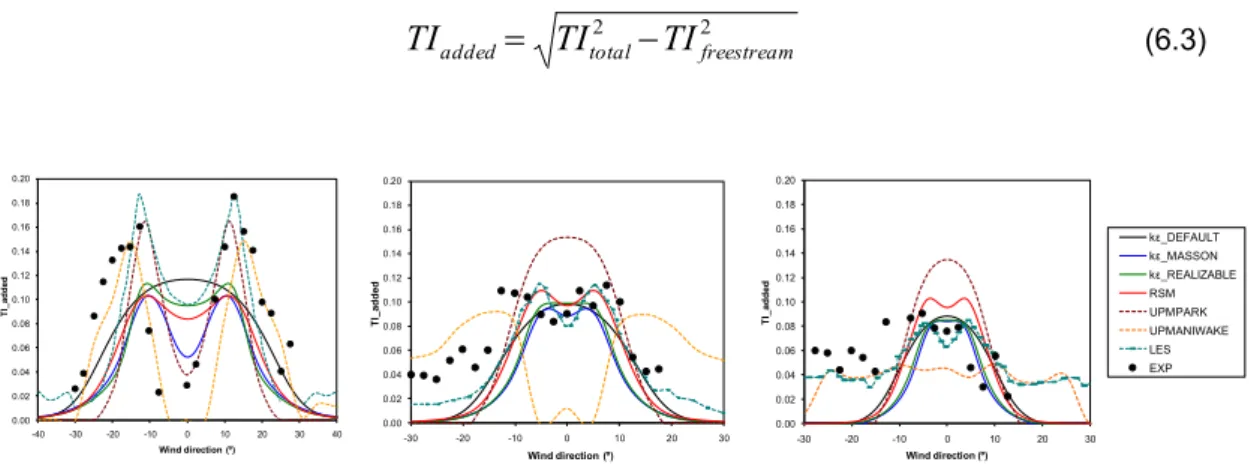
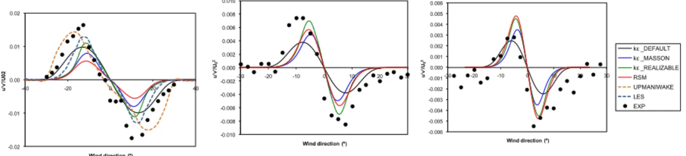
6. Isolated wake analysis ... 52

6.1 Sexbierum experiment ... 52

6.2 Grid independence analysis ... 52

6.3 Turbulence models ... 55

6.4 Results ... 56

6.4 Final remarks ... 60

7. Elliptic modeling of wind farms ... 63

7.1 Description of the elliptic model ... 63

7.2 Reference wind speed. Correction methods ... 64

7.3 Set up of the model. I/O ... 65

7.4 Results ... 66

8. Large offshore wind farms: the semi-parabollic model ... 75

8.1 Description of the semi-parabollic model ... 75

8.2 Set up of the model. I/O ... 77

8.3 Decrease in computational time ... 78

8.4 Results ... 79

8.5 Advantages, shortcomings and further improvements ... 86

9. Wind farms in complex terrain: the hybrid model ... 90

9.1 Wakes in complex terrain ... 90

9.2 Description of the hybrid model ... 92

9.3 Experimental case ... 93

9.4 Numerical set-up ... 94

9.5 Results ... 96

1

1.

Introduction

Wind energy has faced many challenges since its first stage at the early nineties. New technologies have been forced to live under a wide range of different conditions, related to the Atmosphere and Earth. In order to become wind energy a mature technology, Science must make this compatible in quality and price with the remaining mix of energy technologies.

One of the biggest challenges of the science currently consists of trying to explain how modern wind turbines interact between themselves and at the same time with complicated environments where most of the times turbines have to co-exist. This implies that turbine wakes must be correctly analyzed at the engineering phase of every wind farm in order to predict accurately the output power before wind farm construction, to optimize thus layout design and consequently make huge investments profitable in the long term.

As onshore sites in moderate terrain were saturated and occupied, increasingly challenging sites have arisen in order to make wind energy grow, especially in new countries where extreme events or unknown effects have appeared.

Two of these new ‘worlds’ are offshore and complex terrain. The first one supposes currently a large amount of uncertainty in the wind energy community but at the same time, if future plans progress properly; it can be the main source of energy at Northern Europe for the next decade.

Complex terrain environments are older than offshore, and wind turbines have been living with them from a long time ago. Nevertheless, no special focus has been made on this topic during the last years and wind farms have traditionally been designed through conventional tools. Recently the variability of terrain has demonstrated that there is an important impact of topographical features on the wake recovery of wind turbine wakes at the lee sides of hills, leading to the conclusion that new methods, combining wake and terrain effects, are necessary.

All these items show that not only wind turbine designs have to adapt to these two environments (offshore and complex terrain), also wind flow and wake flow models have to be updated in order to ensure that wind farms layout is as optimum as possible.

This means that currently there is an increasing and urgent need to develop new wake models to be used by the wind industry, as established by the Set Plan of the European Union at the 20-20-20 strategy for the next years.

2

Companies use conventional tools for wake modeling based on analytical methods, designed during the nineties for small wind farms in moderately and flat terrain. These tools are very fast, easy to use and extremely useful at the early stage of wind farm design. However, these tools induce lots of uncertainty at the final design phase for offshore or complex terrain environments. That is why new models are intensively demanded in order to reduce this uncertainty and ensure investments.

Nevertheless, wake models must be validated before making any extensive use of them. That is why measurement campaigns are needed to validate and quantify improvements, although data sets to validate wake models are generally much more difficult to get (confidential data sets from SCADA systems), difficult to filter out and also to interpret.

One of the largest European projects where these tasks were extensively carried out was the UPWIND project (funded by the European Union under the 6th Frame Work Programme), running from 2006 to 2010. The UPWIND project represents in fact part of the core work of this PhD thesis for the validation of wake models and represents a unique platform for model evaluation (a wide range of wind farm and CFD models), where the cooperation of a number of groups means that more models can be evaluated on standardized cases.

Preliminary evaluation of the models presented in [1] suggested that standard wind farm models were under-predicting wakes (i.e. over-predicting power output) while computational fluid dynamics models (CFD) were over-predicting wake losses. Some well-known sites for multiple-wake experiments are Horns Rev, Nysted, Middlegrunden, Vindeby and the ECN Wind Turbine Test Site Wieringermeer.

Some other projects such as the ENDOW project [2] in 2004 also made valuable comparative studies between different wake models and experiments and even well-known single-wake experiments, such as the Tjæreborg turbine [3] the Nibe turbine and the Sexbierum measurements [4], had been previously made before UPWIND. The project Wakebench under the IEA Annex 31 has currently brought together to industry and RD centres, to extensively validate wind flow and wind farm models based on a protocol web based methodology. The project runs in the period 2012-2014 and will help to identify the main guidelines on wake metrics together with limits of use of each model.

This PhD thesis proposes, develops and validates a new wake model to solve large wind farms based on the actuator disk approach and the open source CFD solver OpenFOAM for neutral atmosphere, filling thus the gap between engineering and computationally expensive numerical models. This is made by taking the essence of the physics involved in the wake phenomenon inside wind farms and making use of

3

basic information available for wind farms simulation. Formerly parabolic models were proposed to simulate wind farms. Parabolic models solved the flow equations in planes transverse to the main flow direction, and were computationally cheaper but they can be less accurate than elliptic models, that solved the flow equations in the whole flow domain. In this thesis a semiparabolic model for wind farm modeling is proposed that is computationally cheap, gives a good representation of the flow field near the wind turbines, and may also be appropriate for moderately complex terrain.

Since the model is built in a modular way, figure 1.1 describes the main structure of the PhD Thesis such that the reader can have an idea of the relationship between chapters.

The study starts describing the main features of the open source CFD solver OpenFOAM, the reference CFD code used for this work including the most important advantages of this working ‘philosophy’.

Ch. 2 – CFD solver OpenFOAM Ch. 3 – Wind flow model

Ch. 4 –Rotor model Ch 5 –Wake model Ch. 6 – Single-wake analysis Ch. 7 – Wind farm elliptic model Ch. 8 – Offshore:

Semi-parabollic model

Ch. 9 – Complex terrain: Hybrid model

Figure 1.1 Structure of chapters

Once the code is presented, the wind flow model developed for the simulations of the Surface Boundary Layer is presented in chapter 3. This includes all the necessary changes in the boundary conditions as well as grid generation in order to simulate the wind as the fluid surrounding wind turbine wakes.

Chapters 4 makes an overview of rotor models making a clear distinction between models for wind farm design or wind turbine design. It then describes the axial momentum theory and introduces the concept of actuator disk as part of the generalized actuator disk theory. At this stage, the two most important problems are introduced: (1) the estimation of the reference wind speed at each rotor disk and (2) turbulence modeling.

4

This gives the way to chapter 5, where the state-of-the-art in far wake modeling is described: from the analytical or engineering models up to the CFD parabolic and elliptic models, together with the main advantages, shortcomings and limits of use. In chapter 6 the single turbine case is analyzed. The elliptic model based on the actuator disk technique is ready at this point and firstly tested for a single wake case. A review of the different turbulence model parameterizations is made.

Chapter 7 presents the concept of wind farm introducing several wind turbines interacting between themselves and the surrounding. This interaction between turbines implies that the estimation of the reference wind speed is not so obvious and imposes the need for a correction method. Two possible correction methods over the reference wind speed are then proposed and their effect on final power ratio is tested for two wind farms.

Finally, chapters 8 and 9 respectively propose and validate two different adaptations of the general elliptic wake model for the two challenged cases mentioned above:

 A semi-parabollic wake model to solve large offshore wind farms (chapter 8)  An hybrid wake model to solve wind farms in complex terrain (chapter 9) For both cases, results are structured first on analyzing the effect of the semi-parabollic and the hybrid models against the elliptic model and second, once the reference wind estimation is mitigated, on analyzing the effect of using an anisotropic turbulence model instead of an isotropic one.

The thesis ends with the most important conclusions and a proposed a list of further tasks to be continued during the next years. Since the model is based on an open source code that currently represents the reference CFD code for microscale simulation in wind energy, the possibilities to extend it with future developments aligned with industry needs are extremely high making thus the model to be alive in the long term.

5

References

[1] Barthelmie RJ, Frandsen ST, Hansen K, Schepers JG, Rados K, Schlez W, Neubert A, Jensen LE, Neckelmann S. Modelling the impact of wakes on power output at Nysted and Horns Rev. In European Wind Energy Conference and Exhibition, Marseille, 2009.

[2] Barthelmie R, Larsen G, Pryor S, Jørgensen H, Bergström H, Schlez W, Rados K, Lange B, Vølund P, Neckelmann S, Mogensen S, Schepers G, Hegberg T, Folkerts L, MagnussonM. ENDOW(efficient development of offshore wind farms): modelling wake and boundary layer interactions. Wind Energy 2004; 7: 225–245.

[3] Oye S. Tjæreborg wind turbine, first dynamic inflow measurements. Technical Report AFM Notak Vk-189, Technical University of Denmark, 1991.

[4] Cleijne JW. Results of Sexbierum wind farm; single wake measurements. Technical Report TNO-Report 93-082, TNO Institute of Environmental and Energy Technology, 1993.

[5] Bingöl F, Mann J, Larsen GC. Light detection and ranging measurements of wake dynamics. Part I: one-dimensional scanning. Wind Energy 2009; 13: 51–61.

6

2. Open source CFD solver OpenFOAM

2.1 Introduction to OpenFOAM

OpenFoam (Open Field Operation And Manipulation) is one of the most extended open source CFD solvers in the world. It has been applied to almost all the sectors in the industry and extensively validated.

OpenFOAM was developed by H.G. Weller and H. Jasak in 1992 at the Imperial Collegue of London as the main core of its first version called simply FOAM. In 1999, a company called Nabla Ltd. was created in order to develop and give commercial support to FOAM. In 2005, OpenCFD ltd. was born as the official company for the development, maintenance and support of OpenFOAM, now as open source under GNU license.

At the end of 2012, OpenCFD was absorbed by ESI Group, one of the biggest software companies, ensuring thus its survival and open access.

OpenFOAM operates under the GNU license, which means that the distribution and use of the software is free, in order to avoid appropriations.

Each user can extract and derive new codes from other existing one and distribute to any third parties. The main condition is that this distribution must contain the source code apart of the compiled files.

OpenFOAM is based on C++ language and on LINUX operating system. It is basically a huge number of C++ classes linked one to each other in a horizontal way. This makes the programming relatively easy since just those particular classes (few lines) to be modified are selected avoiding thus to review big pieces of code. This makes straightforward the implementation of new turbulence models, boundary conditions, new initialization schemes, etc.

It is fully designed to work in parallel computing and as it is open, it can be parallelized in an unlimited number of cores, making it suitable to be launched in multi-core workstations or even in clusters of computers. Preliminary analysis have demonstrated that OpenFOAM can be scalable up to 1000 cores, although this can vary depending on the type of mesh, numerical schemes or type of processor used in the analysis.

2.2 Installation

OpenFOAM can be easily installed from the Synaptic tools or following the instructions from the official web page (www.openfoam.com). In both cases the code is already compiled. The source pack can also be downloaded and specifically compiled. The code

7

must be installed using root permissions. It is normally installed and located at the opt/ folder.

Current version (2013) is OpenFOAM 2.2. Nevertheless, OpenFOAM 1.7.1 [1] was used for this work since most of the libraries were developed at the time when this version of the code was released.

Before start using it, the bashrc file of OpenFOAM has to be sourced from the .bashrc (file with the definition of the environment variables of the local user) in order to set-up all the variables included in the code. This is made by adding the line at the end of the .bashrc file:

. /opt/openfoam171/etc/bashrc

2.3 Applications and libraries

Once installed, the compiled code in the opt/ folder is the official one and it cannot be modified by any user. It contains mainly two types of compiled files:

 Applications, like solvers of partial differential equations (PDE), such as systems Navier Stokes equations in different regimes and utilities for pre-processing (operations on grids) and post-processing.

Applications have an exe extension and they are located at the applications/bin folder. Although most of the solvers are focused on fluid dynamics (including turbulence, heat transfer, multiphase states…), OpenFOAM contains some other solvers useful for the solution of problems on structural analysis, electromagnetism or financial analysis. The main solver used in this work is simpleFoam, which is focused on the solution of incompressible turbulent steady-state flow. It solves thus the continuity and momentum equations together with any turbulence model. There are many other solvers available for incompressible flows such as pisoFoam specifically for transient problems or icoFoam for transient laminar flow of Newtonian fluids. Other families of solvers are dedicated for the solution of compressible flows, multiphase flows, LES and DNS cases, combustion problems, particle-tracking flows and heat transfer and buoyancy-driven flows.

8 o Preprocessing of grids: generation of grid, conversion of formats from other grid generators and solvers such as FLUENT, plot3D or gmsh and manipulation of grid by means of different operations (extrusion, separation of cells, rotation, etc.)

o Post-processing of converged cases: conversion of fields into Paraview format for graphical post or access to values of different variables at points, lines or surfaces.

 Libraries, such as turbulence models, boundary conditions, source terms, etc. They have and so extension and are located at the /lib folder.

In all the cases, the user can interact with the code by means of dictionaries, which are text files (identified with the Dict suffix) where the corresponding inlet values of the parameters can be introduced such as the mesh description, the number of subdomains to be used, the type of numerical schemes, etc. This is described on the next section.

2.4 Folder structure in OpenFOAM

The solution of any case in OpenFOAM is always structured in 3 different folders: Folder: Constant/

It contains all the information to remain constant along the solution of the CFD case: A. The mesh description contained in the polymesh/ folder. This information is

described through text files containing, among others, the coordinates of nodes and their connectivity.

B. Turbulence model (for laminar flow, it is simply deactivated). This is done at the

RASProperties file (RANS simulations), where the name of the model and the values of the set of constants are specified.

C. Properties of the fluid, described at the transportProperties file. Folder: N/

It contains the description of the boundary and internal fields related to the different variables involved in the calculation: wind speed, turbulence quantities (k, ε and µt)

and pressure. Each variable is described in a different text file including the boundary and internal fields.

9

In the case of initial conditions (N=0), the corresponding value of each variable are assigned to the internal field, whereas for intermediate solution fields at different iterations of the calculation (folders N=100, 200, etc.), the files inside contain the description of the internal field at that iteration. Boundary conditions are constant for any considered iteration.

In case of steady-state calculations N is equal to the iteration number, whereas in transit calculations, N corresponds to the considered time step. At this Thesis, all the calculations shown will be steady-state.

System/

The system folder contains those parameters related to all the numerical aspects of each simulation, including discretization schemes (fvSchemes file), type of solvers used for the different variables (fvSolution file), parallelization algorithms (decomposeParDict) and simulation controls (ControlDict).

At this Thesis, the PBiCG (preconditioned bi-conjugate gradient) solver is used for the solution of wind speed, k and ε) and the GAMG (generalised geometric-algebraic multi-grid) solver for the solution of pressure. Numerical schemes are first and second order upwind whereas the decomposition method to be used is metis or scotch for parallel calculations.

The analytical post-processing is also controlled from the system/ folder, setting up, for example the coordinates of point, lines or surfaces to be used for extracting the variables. This is made through the dictionary specified in the sampleDict file.

2.5 Simulation run

Once the simulation has been set-up, it can be easily launched from the root path of the case.

In the case that of serial simulation is to be launched (one single processor), the number of the solver can be typed directly, in this case simpleFoam.

In case of parallel simulation, the domain and the corresponding fields have to be first decomposed (according to the specifications in the decomposeparDict file). Obviously, the maximum number of subdomains will depend on the number of available cores at the workstation or cluster used for the calculation.

10

Once this is done, the simulation can be launched for all subdomains. In the case that a parallel simulation wants to be run in N nodes, this is done by means of the mpi library using the expression.

mpirun –np N simpleFoam .parallel

Once the simulation has finished, the domain has to be reconstructed before the post-processing. This is through the reconstructPar utility.

In both cases, the residuals of the simulation can be monitored from the screen or re-directed into an external file. This last option is quite useful since the residuals can be plotted in order to ensure convergence.

2.6 Post-processing

Once the simulation is considered as converged, an analytical post processing can be done at the corresponding points, lines or surfaces of interest. A graphical post can also be carried out by exporting the results into the open source post-processing code Paraview, developed by Sandia Laboratories.

2.7 Other information sources

Although the official release of the code (together with the official users and programmers guide) can be downloaded from the official web page, there are some other sources of information that are utilized by most of the users:

 Non-official web page: openfoamwiki.net

It contains information on training courses and workshops, additional documentation and downloadable open source software as well as tips and tricks.

 Since not all the information is included at the users guide, dedicated forums on OpenFOAM users result very helpful when some problem arises. One of the most extended forums is cfd-online which contains forums for the most extended CFD codes currently on use. In particular for OpenFOAM, the link www.openfoam.cfd-online.com/forum offers quick and helpful answers to many questions that most of the times have previouslyraised to other users.

This networking way of collaborative work makes the development of the code to extend very quickly since all the users keep in contact through the different forums and workshops.

11

Active communities of users have been created in some countries such as Germany and the Netherlands.

Recently a transversal community of users especially focused on wind energy has been created. A first symposium on OpenFOAM in wind energy was held in March 2013 in Oldenburg (Germany), where one of the main contributions of this Thesis was presented [2].

Most of the applications are focused for the moment on wind flow simulation on the ABL and rotor and blades aerodynamics. This will enable in the following years a rapid expansion of the OpenFOAM as the reference open source CFD solver in the wind energy sector worldwide.

References

*1+ OpenCFD, “OpenFOAM: The Open Source CFD Toolbox – Programmer’s Guide v1.7”, 2010

*2+ Cabezon D., Migoya E., Crespo A., “A semi-parabolized wake model for large offshore wind farms based on the open source CFD solver OpenFOAM”, Journal of Informatics and Mathematics, accepted for publication

12

1.

Surface Boundary Layer Flow Modeling

Computational Fluid Dynamics (CFD) techniques have become a useful and extended tool for many industrial sectors where simulation is extremely necessary at preliminary designing steps.

Wind energy is one of these sectors and CFD has been applied during the last years in almost all of the fields, from air flow inside the atmosphere boundary layer to air flow around blades and rotor.

One of the main applications of CFD to wind energy has been focused on wind and energy assessment studies at particular sites in order to reduce the uncertainty in the estimation of long term energy of wind farms. Some tools have been implemented with this purpose as an alternative to classical wind flow linear models [1].

In the same way, new wake models based on CFD methods have been developed also as an alternative to the classical engineering methods. These engineering methods are useful for designing and optimizing wind farms, but not to estimate the mean and turbulent quantities of the flow field in a more detailed way at the surroundings of the wind turbines. For estimating accurately the flow characteristics in the wake, both near and far from the turbine, more sophisticated methods are necessary, methods that rely on the solution of the partial differential equations of the fluid flows, mostly known as the Navier–Stokes equations, and on a suitable model to describe the aerodynamics of wind turbine.

The flow of air without heat sources is generally considered as incompressible if local Mach number does not exceed 0.3. In the standard atmosphere at sea level this corresponds to a flow velocity of approximately 100 m/s. However, the velocities in the wake remain much lower and for wind farm applications incompressibility is a valid assumption. This is thus a reasonable hypothesis to assume, since the velocities upstream and downstream of a turbine placed in the atmosphere are typically in the range of 5–25 ms-1. Only when calculating the aerodynamics at blade tips that compressibility effects may be important in some cases.

It has also to be assumed that atmospheric conditions are near neutral, so that buoyancy due to density variations associated to thermal effects is negligible. Otherwise, although density variations are in any case small compared to density itself, they may be relevant dynamically, and are usually taken into account through the so called Boussinesq approximation. Neutral conditions correspond to situations where mechanical effects dominate over heat transfer effects; these may correspond to cloudy days with high winds [2]. Although wind energy usually corresponds to high winds, that does not necessarily mean that thermal effects can be neglected, and several authors have studied the influence of atmospheric stability in wake characteristics, see for example Crespo et al.[3,4] and the review papers [5] and Vermeer et al. [6].

13 3.1 The incompressible Navier-Stokes equations

Since in most calculations of wind turbine wakes the rotor is not modeled directly (which will be discussed later), the incompressible Navier-Stokes equations are a suitable model to describe the aerodynamics of wind turbine wakes:

(3.1)

Where represents the gradient operator and represents the laplacian operator.

The previous equation is supplemented with initial and boundary conditions (described later in this chapter).

The most common approach in wind engineering to deal with turbulent flows is the Reynolds Averaged Navier-Stokes (RANS) approach. The Reynolds decomposition ( is applied to the variables  of the time-dependent Navier Stokes equations (Eqs. 3.1 to 3.2).

The governing equations for an incompressible fluid of density ρ and steady-state with Cartesian notation are the continuity equation (Eq. 3.3) and the Momentum Equation (Eq. 3.4). The vector form of the equations can be substituted by the Einstein summation as:

The result of doing the Reynolds decomposition is the existence of six new terms composing the Reynolds stress tensor. This tensor represents the average flow of momentum (per unit area) passing through a finite volume surrounding a fluid particle due to turbulent fluctuations. The Reynolds stresses can then be interpreted as turbulent diffusive forces.

In order to close the system of equations and due to its non linear nature, the Reynolds stress tensor has to be solved through a turbulence closure scheme. One of

14

the most extended schemes is related to the widely adopted approach of the Boussinesq hypothesis [7]:

where µt is the turbulent viscosity and k= the turbulent kinetic energy.

As the flow is considered incompressible, the gravitational force can be absorbed in the pressure term [8]. The term is also absorbed in the pressure term (Eq. 3.6) in the form of reduced pressure.

Besides, in turbulent regime, and µ is neglected.

Concerning Coriolis force, wind turbines considered in this work are between 50 and 100 meters height and consequently located inside the Surface Boundary Layer (SBL), so that this force will not be taken into account.

Finally, the continuity and momentum equations become:

3.2 Turbulence modeling: isotropy and anisotropy

Since atmospheric flow is fully turbulent, equations must include a turbulent closure scheme that takes fluctuations of variables into account. This implies, among other things, to specifically determine the value of turbulent viscosity.

This way, an ideal model should introduce the minimum amount of complexity and at the same time include the essence of the physics [9]. In fact, practical engineering models are mostly turbulent, and simple closure models are necessary.

Turbulence has a strongly rotational nature so it must be three dimensional, with multitude of length scales and time dependence.

15

A large number of turbulence models have been constructed in the last decades, since the simple algebraic mixing length model to a complete solution of the Navier Stokes equation.

Turbulence kinetic energy is transferred on average from larger eddies to smaller eddies until it is dissipated into heat through the action of molecular viscosity.

An N-equations model means a model requiring solution for N additional differential transport equations in addition to conservation of mass and momentum equation (3.7) and (3.8).

This section will discuss the mostly extended and practical methodologies in turbulence modeling for wind turbine wakes based on RANS models.

3.2.1 Isotropic model k-ε

In wind engineering applications, k-ε turbulent model has been largely used *10-12] for the simulation of the surface boundary layer, due its robustness economy and its relative simplicity and accuracy for a wide range of flows.

The first variable to consider is the turbulent kinetic energy considered as the kinetic energy of the turbulent fluctuations, also called TKE or k, already introduced in eq. (3.5). The second variable is the turbulent dissipation rate (ε) and determines, together with k, the scale of turbulence, that is of the order of _k3/2/_.

The Jones and Launder k-ε model [13] is one of the most popular for turbulence modeling. The transport equations for these two magnitudes are:

Where Pk is the turbulent production term:

k and ε are related by the above presented turbulent viscosity µt

16

Cµ=0.09, C1ε=1.44, C2ε=1.92, σk=1, σε=1.3 (3.13)

Some derivations from the standard k-ε turbulence model have been proposed by different authors during the last years, such as the Realizable model [14] and the RNG model [15].

In both cases, every modification attempts to mitigate the overestimation of the turbulence viscosity produced by the standard model (which is the main drawback) especially at high curvature areas where intensive velocity gradients occur.

3.2.2 Anisotropic model RSM (Reynolds Stress Tensor)

Another approach of simulating the anisotropy of turbulence in the atmosphere is to solve all the terms in the Reynolds Stress Tensor, through the introduction of seven extra equations into the system, configuring the so-called Reynolds Stress Model (RSM). Among the different versions existing in the literature of RSM, the model proposed by Gibson and Launder [16] is used because it is the most extended and it has proven accuracy for many flow cases.

The model takes into account all the effects derived from rapid changes at the main strain tensor in a more rigorous way than 1 or 2 equations turbulence models. It has a great potential when carrying out simulations for complex flows, although it implies an increase in computational time.

Nevertheless, the accuracy of RSM is still limited to the closure hypothesis used at the transport equations of the stress tensor, particularly those referred to the turbulent diffusion, pressure gradient and dissipation. The rest of the terms of the equations (convection, molecular diffusion and production) do not require to be specifically modeled.

Besides the seven equations prescribed for the Reynolds stress tensor, the RSM model solves the k and ε equations as well in a similar way to the standard k-ε model. The value of k obtained from this model is used for the definition of the Reynolds stress values at the wall adjacent cells using a local coordinate system.

The use of the RSM model to simulate turbulence flow in the atmospheric boundary layer is not quite extended for wind engineering applications. Nevertheless, it represents a step forward in comparison to the isotropic models since it solves the already known anisotropy of atmospheric flow still using the RANS approach and avoiding expensive computational models such as LES, at least for operational use. All the presented turbulence models are available in OpenFOAM and they have been modified appropriately where necessary.

17 3.3 Solution of SBL flow in OpenFOAM

The atmospheric boundary layer (ABL) is defined as the part of the troposphere directly influenced by the presence of Earth surface and responding to its forcing actions such as frictional, drag, evaporation, heat transfer, pollutant emission and terrain induced flow modification [17]. These forces give rise to the main characteristic of the ABL: turbulence. Meteorological phenomena take place in this layer with different time scales.

Typically the ABL is divided in three sub-layers: the surface boundary layer (SBL), the mixed layer and the entrainment zone.

The surface boundary layer is located at the bottom of the ABL and close to the surface. Its typical height is 10% of total and it is characterized by high vertical gradients of wind speed, humidity and temperature. Nevertheless, this height can vary with local meteorological conditions (heating from the ground and thermal stratification) along the time of the day and the year.

The mixed layer, turbulence is mainly due to heat transfer between warm ground surface and irradiative cooling from the top of mixed layer. The entrainment zone is a stable layer at the top of the mixed layer acting as a lid restraining the domain of turbulence [11].

For energy applications, the most interesting sub-layer is the SBL, where wind turbines are installed. For simplicity, Coriolis effects and buoyancy and thermal effects will be neglected in this work.

The CFD solver OpenFOAM was adapted in order to solve air flow inside the surface boundary layer, for complex terrain and also for flat cases. All the default libraries and solvers were adapted to be used as a wind flow solver.

The solver is complemented through the grid generator WindMesh developed by the Barcelona Supercomputing Center (BSC) for complex terrain surfaces. Generated grids are fully structured and completely adapted to be run with OpenFOAM.

The model is adapted for the simulation of wind speed and turbulence based on the Monin-Obukhov theory [2] and on the Richards and Hoxey computational approach [18].

The wind flow model has been validated at several sites, such as the Bolund blind test [15, 16], showing very accurate results.

18 3.3.1 Boundary conditions (k-ε)

Although the set of equations presented before provides a complete model for the description of turbulent flows, it is not easily solved. The difficulty associated with turbulent flows is the presence of the non-linear convective term, which creates a wide range of time and length scales [2].

a. Inlet

The computational approach of Richard and Hoxey [18] ensures that for a steady-state, neutral, incompressible and horizontally homogeneous flow and assuming constant pressure and shear stress, the following wind speed and turbulence profiles are exact solutions of the flow equations for a k-ε turbulence closure:

where

= friction velocity (m/s) z0 = roughness length (m)

κ = von Karman constant (=0.4187) zgr = height (a.s.l.) of ground

Cµ = constant of the k-ε turbulence model

Additionally, constants of the k-ε turbulence model must satisfy the following equation together with the previous profiles:

Different set of constants for the k-ε turbulence model have been proposed. The measurements made by Panofsky et. al. [2] leads to a nice description of the

19

atmospheric turbulence. The following set of constants fulfills Panofsky proposal as well as equation (21):

Cµ=0.0333, Cε1=1.181, Cε2=1.92, σk=1.0, σε=1.3 (3.18)

This analysis has been extended by Crespo and Hernández [4] to non neutral atmospheres.

b. Ground

Together with the inlet boundary, the ground is the most critical boundary in wind flow simulation since it has to ensure the equilibrium of the inlet profiles along the domain and avoid momentum losses. As it will be shown, there are several ways of getting this objective.

Most wall treatments are originally derived from the logarithmic law for rough walls, also called law of the wall (Eq. 3.19) modified for rough surfaces, described in its most generic form as:

with

u = mean velocity tangential to the wall = wall friction velocity

ν = kinematic viscosity u+=wall velocity (=u/ )

z+=wall coordinate (= z/ν) and B=5.2

The modifications for rough surfaces were made mainly by Nikuradse (1953) for flow in rough surfaces introducing the equivalent sand-grain roughness ks.

Nikuradse’s experiment showed that near a rough wall, the mean velocity distribution has the same trend as a smooth wall but shows different intercept in a semi-logarithmic scale (Fig. 3.1).

20 Figure 3.1 Law of the wall for smooth and sand-grain roughened surfaces with the dimensionless

sand-grain roughness ks+ as a parameter

This difference is a function of the dimensionless sand-grain roughness height :

In the current case, the terrain is fully rough ( so the laminar sublayer is deleted due to the no-influence of the molecular viscosity to the flow.

The term ‘‘sand-grain-roughness wall functions’’ is here introduced, which refers to standard wall functions modified for roughness based on experiments with sand-grain roughness, also called kS-type wall functions. The ktype wall function for mean velocity

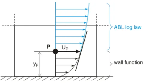
is obtained by replacing u and z in Eq. (3.19) by their values in the centre point P of the wall-adjacent cell: uP and zP.

Several CFD codes (such as Fluent, which defines the wind speed at the wall adjacent cell or OpenFOAM, which defines the equivalent turbulent viscosity µt) use slightly

different kS-type wall functions than Eq. (3.19).

In this case, the rough wall functions and non-slip conditions for wind speed are used. Essentially two wall functions for the turbulent viscosity µt and the turbulent

dissipation rate ε are offered by OpenFOAM: nutRoughWallFunction and

21

Wall functions have a major importance for near-wall modeling.

nutRoughWallFunction is the function used by OpenFOAM to model near-wall behavior.

Changing u and z by uP and zP (value of wind speed at the near wall cell and the

distance to the wall value, respectively), the wall function used is:

Where E is the smooth wall constant (=9.793) and represents the roughness modification for roughness walls.

Since in wind engineering, , then equation (3.25) becomes:

The challenge is then to make equivalent the velocity of the law-of-the-wall and the SBL log-law, in order to preserve the same roughness length and consequently prevent the presence of an internal boundary layer that could deteriorate the flow homogeneity (Fig. 3.2).

22

Blocken et. al. [21] proposed several solutions in order to mitigate this problem. One of them consisted of matching equations (3.14) and (3.22) to ensure continuity of both functions as well as their first derivative.

The following relationship was thus obtained (considering zgr=0):

With

If ks is maximized ( , then:

Such that, knowing the value of z0 and zp at the wall, the value of Cs as specified in

equation (3.24) can be used in order to ensure equilibrium.

c. Outlet and lateral

When analyzing the free-stream flow, the outlet and lateral boundary has to be placed as far as possible such that local flow is in equilibrium and fully developed. All the variables are then set as zeroGradient, excepting µt which is recalculated from the k

and ε values at the nodes.

d. Top

According to Richards and Hoxey approach [13] one of the conditions in order to ensure the existence of a homogeneous, steady and incompressible flow, the shear stress τw must be constant along all the domain.

One possible solution would then be to fix the shear stress value at the top boundary and the other one, adopted here, consists of fixing the inlet values of wind speed and turbulence quantities at a height z=ztop.

In order to ensure the equilibrium of vertical profiles, a flat terrain case was launched in a virtual wind tunnel mode with dimensions of 1000 m in the axial direction and 100 m in the transversal and vertical directions [10]. As it observed in figure 3.3 both the wind speed and turbulence kinetic energy profiles are maintained equal, as expected, between the inlet and the outlet of the domain.

23

Figure 3.3 Simulation of the surface boundary layer flow over flat terrain based on the kε turbulence model

3.3.2 Boundary conditions (RSM)

In the same way, similar boundary conditions have to be applied when the RSM model is used. The main difference is that different values for the components of the Reynolds stress tensor have to be assigned at the entrance of the domain.

Since the tensor is symmetric, only 6 difference values have to be assigned. From the measurements by Panofsky et. al .[2] at the SBL, the components of the tensor can be specified as:

, (3.25)

The same value of the tensor components is applied at the top boundary and a zeroGradient condition is applied at the top, lateral and ground boundaries.

Since the RSM model runs in parallel a k-ε turbulence model, similar boundary conditions are applied for k, ε and µt as for the previous standard k-ε turbulence

model.

It has to be mentioned that the application of the RSM turbulence model to wind flow and wakes modeling is still for the current state-of-the-art in an experimental phase so that final results should always be considered as preliminary. This is confirmed from figure 3.4 where vertical profiles at the inlet and outlet of a similar flat domain are not identical, leading to the conclusion that they are not in fully equilibrium with the wall. This implies the need to adjust a set of constants for the turbulence model that ensure the equilibrium of them with the previous inlet profiles and the boundary condition prescribed at the wall.

24

Figure 3.4 Simulation of the surface boundary layer flow over flat terrain baed on the RSM turbulence model

25 References

[1]Gravdahl A., Meissner C., Weir D., CFD Validation. A simple approach with Windsim. Proceedings of the EWEA Brussels, 2011.

[2] Panofsky H.A., Dutton J.A., Atmospheric Turbulence, Models and Methods for Engineering Applications, Wiley & Sons, 1984.

[3] Crespo A, Manuel F, Moreno D, Fraga E, Hern!andez J. Numerical analysis of wind turbine wakes. In: Bergeles G, Chadjivassiliadis J, editors. Proceedings of the Delphi Workshop on Wind Energy Applications, Delphi, Greece, 1985. p. 15–25.

[4] Crespo A, Hernández J. Numerical modelling of the flow field in a wind turbine wake, Proceedings of the 3rd Joint ASCE/ASME Mechanics Conference, Forum on Turbulent Flows. ASME, FED-vol. 76, La Jolla, CA, USA, 1989; 121–7.

[5] Crespo A, Hernández J, Frandsen S. A survey of modelling methods for wind-turbine wakes and wind farms. Wind Energy 1999; 2: 1–24.

[6] Vermeer LJ, et. al. Wind turbine wake aerodynamics. Progress in Aerospace Sciences 2003; 39: 467– 510.

[7] Versteeg, H. and W. Malalasekera, 2007. An introduction to Computational Fluid Dynamics, The Finite Volume Method. 2 edition. Pearson Education Limited.

[8] Sørensen JN, Kock CW. A model for unsteady rotor aerodynamics. Journal of Wind Engineering and Industrial Aerodynamics 1995; 58: 259–275.

[9] Wilcox DC. Turbulence Modeling in CFD. DCW Industries: La Canada, 2006.

*10+ Sanz J., Cabezón D., Martí I., Patilla P., van Beeck J., “Numerical CFD modelling of non-neutral atmospheric boundary layers for offshore wind resource assessment based on Monin-Obukhov theory”, EWEC 2008 scientific proceedings, Brussels, Belgium, April 2008.

[11] Palma, J., F.A. Castro, L.F. Ribeiro, A.H. Rodrigues, and A.P.Pinto. 2008. “ Linear and nonlinear models in wind resource assessment and wind turbine micro-siting in complex terrain ”. Journal of Wind Engineering and Industrial Aerodynamics, p. 2308-2326.

[12] El Kasmin A., Masson C., "An extended k- model for turbulent flow through horizontal-axis wind turbines", J. Wind Engineering and Industrial Aerodynamics Vol. 96, pp 103-122, 2008

[13]Launder B.E. and Spalding D.B., "Lectures in Mathematical Models of Turbulence", Academic Press, London, England, 1972

[14+ Shih T., Liou W., et. al., "A new kε eddy viscosity model for high Reynolds number turbulent flows", Journal of Computers Fluids, Vol. 24, pp. 227-238, 1995

[15] Yakhot, V. and S. A. Orszag. 1986. Renormalization group analysis of turbulence. I. Basic theory. Journal of Scientific Computing, vol. 1, no. 1, p. 3–51.

[16] Gibson M.M. and Launder B. E. “Ground Effects on Pressure Fluctuations in the Atmospheric Boundary Layer” J. Fluid Mech., 86:491–511, 1978

[17] Stull RB. An Introduction to Boundary Layer Meteorology. Kluwer Academic Publishers: Dordrecht, 1988

[18] Richards P.J., Hoxey R.P., Appropriate boundary conditions for computational wind engineering models using the k-ε turbulence model, Journal of Wind Engineering and Industrial Aerodynamics 46-47 (1993), 145- 153.

[19] Benchmann, A., J. Berg, M.S. Courtney, H.S. Jorgensen, J. Mann, and N.N. Sorensen. 2009b. The bolund experiment: Blind comparison of flow models.

26 *20+ Cabezón D., Sumner J., García B., Sanz Rodrigo J., Masson C., “RANS simulations of wind flow at the Bolund experiment”, EWEC 2011 scientific proceedings, Brussels, Belgium, March 2011

[21] Blocken, B., Stathopoulos, T., Carmeliet J., CFD simulation of the atmospheric boundary layer – wall function problems. Atmospheric and Environment 41-2, 2007, 238-252.

[22] Porté-Agel F, Lu H, Wu Y. A large-eddy simulation framework for wind energy applications. In Fifth International Symposium on Computational Wind Engineering, Chapel Hill, 2010.

[23] Davidson PA. Turbulence—An Introduction for Scientists and Engineers. Oxford University Press: Oxford, 2004

27

4.

Rotor modeling

4.1 Overview of rotor models. Wind farm vs wind turbine design

The representation of a wind turbine can be approached by a wide range of models, from the simplest to the most sophisticated methods. This level of complexity mostly depends on the objective of the study and on the amount of available information. Since their main focus is on wind farm design, wind farm models represent wind turbines in a simple way. These models are feasible to simulate the far wake of large wind farms (table 4.1). On the other hand, there are some other specific rotor models mainly focused on the aerodynamic analysis of rotor components at the phase of wind turbine design (table 4.2).

Wind farm models can be broadly separated into kinematic models (also called analytical or engineering) and the more complex (but also more time consuming) field or CFD models.

The first and simplest approach of kinematic modeling is an analytical method that exploits the self similar nature of the far wake to obtain expressions for the wake velocity deficit and turbulence intensity.

All of them are focused in wind farm designed and, together with the CFD parabolic and elliptic models, can be summarized at table 4.1. These models will be in fact the main objective of this Thesis.

The field methods, the generalized actuator disk method and the direct method, are relatively new and are commonly called computational fluid dynamics (CFD) methods. Some of them have been combined with models in table 4.2 (such as the BEM model) with significant improvements. In this chapter, a description of models in table 4.1 is made making special emphasis on the actuator disk approach as it will be the main model used of this work.

Method Blade model Wake model

Kinematic Ct coefficient Self-similar solutions

CFD Parabollic Velocity deficits and turbulence addings Parabolic Navier Stokes

CFD Elliptic + Generalized ADM AD, AS, AL Volume mesh, Euler/RANS/LES

Table 4.1 –Rotor and wake models focused on wind farm design [AD=Actuator Disk, AS = Actuator Surface, AL=Actuator Line]

28

Method Blade model Wake model

CFD-BEM coupling ADM + blade element Quasi 1D momentum theory

Vortex lattice, vortex particle lifting line/surface + blade element Free/fixed vorticity sheet

Panels Surface mesh Free/fixed vorticity sheet

Direct Volume mesh Volume mesh, Euler/RANS/LES

Table 4.2 –Rotor and wake models focused on wind turbine design

Models in table 4.2 are focused on wind turbine and rotor design and need always as input specific information related to the rotor geometry such as the aerodynamic features of the profiles.

Some of them, such as the Blade Element Momentum Theory (BEM), uses a global momentum balance together with a 2D blade element approach to calculate aerodynamic blade characteristics.

The vortex-lattice and vortex-particle methods assume inviscid, incompressible flow and describe it with vorticity concentrated in sheets or particles.

In the same way, panel method similarly describes an inviscid flow field, but the blade geometry is taken into account more accurately and viscous effects can be included in a boundary-layer code.

4.2 Axial momentum theory

Since a wind turbine extracts energy from the wind, a fluid element passing through the rotor loses part of its kinetic energy. The flow through a wind turbine slows down gradually from some upstream value u0 to an average value far downstream in the

wake uw. The static pressure increases from its upstream value p0 to a value pd+ just in

front of the disk and then drops suddenly behind the disk to a value pd-. This pressure

difference across the disk is associated to the axial force exerted by the disk. The pressure gradually recovers in the wake to the free-stream value p0, as it is seen in

figure 4.1.

29

Using this process of energy extraction by the actuator disk as a black box, a number of analytical relationships can be derived using the equations of conservation of mass, momentum and energy (incompressible flow) [2]:

Continuity: m=ρ·A0·u0= ρ·Ad·ud= ρ·Aw·uw (4.1)

Force on disk: F=m·(u0-uw)=(p+d-p-d)·Ad (4.2)

Energy extracted: E=0.5·m· (u02-uw2) (4.3)

If the kinetic energy associated to the flow rotation is neglected, the energy extracted per unit time gives the power: P=0.5·m·(u02-uw2). This power is equal to the power

performed by the force T acting on the disk, P=T·ud=m·(u0-uw)·ud.

Equating these two expressions leads to:

ud=0.5· (u0+uw) (4.4)

In order to compare the power of different wind turbines the power coefficient Cp is used, defined by:

(4.5) i.e. the power is non-dimensionalized by the wind speed and the rotor swept area. The expression for the power coefficient becomes

CP = 0.5(u0+uw)(u02-uw2)/u03 = 0.5(1+b)(1-b2) = 4a(1-a)2 (4.6)

Where a=1-(ud/u0) is the axial induction factor and b=uw/u0, hence a=(1-b)/2. The

optimal Cp is found at a=b=1/3, such that CPmax=16/27=0.59, known as the Bet limit. It

shows that, within the assumptions of the derivation, a maximum of 59% of the wind energy can be converted into mechanical power. A similar definition exists for the thrust coefficient CT,

(4.7) At optimal CP,the thrust coefficientCT is equal to 8/9. Note that, due to the decrease in

velocity behind the turbine, uw<ud, so that Aw>Ad, leading to the expansion of the

30 4.3 Generalized actuator disk technique

CFD rotor models can be summarized in two different groups: a simplified version where the rotor can be represented as an actuator disk in elliptic models (also approached by an actuator line or an actuator surface) over the incoming air or as a more sophisticated direct approach, where the blades are represented specifically in the mesh.

The first approach, using actuator disk, will be the focus of this work since it is the most extended and practical model to simulate entire wind farms. The approximation of rotor as an actuator disk can be more or less sophisticated depending on the level of available information.

If the available information includes the general data from manufacturer (power curve and Ct curves), then just the axial component of the body force can be assigned over the rotor disk. The actuator disk exerts thus a force on the flow, acting as a momentum sink. This force Si is explicitly added to the momentum equation (3.8) as exposed in

previous chapter, giving as a result equation (4.8):

Currently, three different approaches for prescribing the force term F exist: the actuator disk, the actuator line and the actuator surface models (see Figure 4.2).

Figure 4.2 Actuator disk (AD), actuator lines (AL) or actuator surface (AS) [3]

From the linear momentum theory, it can be derived that the axial force from which the wind turbine extracts the kinetic energy from the incoming air flow, is just a function of the local induction factor or alternatively, of the thrust coefficient for the corresponding upstream wind speed [4-6]. The wind turbine is thus considered as an actuator disk upon which a uniform or non-uniform distribution of axial forces, defined as momentum sink terms, is applied. For the case of a uniform loaded rotor, local axial forces can be prescribed over the disk area as:

31

(4.9) where:

A = rotor area (m2)

Vref = upstream wind speed (m/s), obtained at this case from the upstream mast

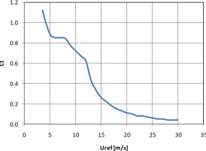
Ct = thrust coefficient, obtained from the [Ct – velocity] curve (as showed in figure 4.3)

for the corresponding value of Vref

ρ = air density (kg/m3) 0.0 0.2 0.4 0.6 0.8 1.0 1.2 0 5 10 15 20 25 30 35 Ct Uref [m/s]

Figure 4.3 Example of a Thrust Coefficient - Uref Curve

The local prescribed force is to be applied on a volume of cells defining the rotor in units of force per cubic meter (N/m3).

Considering X as axial direction, Y as transversal and Z as vertical, the rotor disk can represented as it is illustrated in the figure 4.4: