A Large Scale Evaluation of Distributional Semantic Models:
Parameters, Interactions and Model Selection
Gabriella Lapesa2,1 1Universit¨at Osnabr¨uck
Institut f¨ur Kognitionswissenschaft Albrechtstr. 28, Osnabr¨uck, Germany
Stefan Evert2 2FAU Erlangen-N¨urnberg
Professur f¨ur Korpuslinguistik Bismarckstr. 6, Erlangen, Germany
Abstract
This paper presents the results of a large-scale evaluation study of window-based Distribu-tional Semantic Models on a wide variety of tasks. Our study combines a broad coverage of model parameters with a model selection methodology that is robust to overfitting and able to capture parameter interactions. We show that our strategy allows us to identify pa-rameter configurations that achieve good per-formance across different datasets and tasks1.
1 Introduction
Distributional Semantic Models (DSMs) are em-ployed to produce semantic representations of words from co-occurrence patterns in texts or documents (Sahlgren, 2006; Turney and Pantel, 2010). Build-ing on the Distributional Hypothesis (Harris, 1954), DSMs quantify the amount of meaning shared by words as the degree of overlap of the sets of contexts in which they occur.
A widely used approach operationalizes the set of contexts as co-occurrences with other words within a certain window (e.g., 5 words). A window-based DSM can be represented as a co-occurrence matrix in which rows correspond to target words, columns correspond to context words, and cells store the co-occurrence frequencies of target words and context words. The co-occurrence information is usually weighted by some scoring function and the rows of the matrix are normalized. Since the co-occurrence
1The analysis presented in this paper is complemented by
supplementary materials, which are available for download at http://www.linguistik.fau.de/dsmeval/. This page will also be kept up to date with the results of follow-up experiments.
matrix tends to be very large and sparsely popu-lated, dimensionality reduction techniques are often used to obtain a more compact representation. Lan-dauer and Dumais (1997) claim that dimensionality reduction also improves the semantic representation encoded in the co-occurrence matrix. Finally, dis-tances between the row vectors of the matrix are computed and – according to the Distributional Hy-pothesis – interpreted as a correlate of the semantic similarities between the corresponding target words. The construction and use of a DSM involves many design choices, such as: selection of a source cor-pus, size of the co-occurrence window; choice of a suitable scoring function, possibly combined with an additional transformation; whether to apply dimen-sionality reduction, and the number of reduced di-mensions; metric for measuring distances between vectors. Different design choices – technically, the DSM parameters – can result in quite different sim-ilarities for the same words (Sahlgren, 2006).
DSMs have already proven successful in model-ing lexical meanmodel-ing: they have been applied in Natu-ral Language Processing (Sch¨utze, 1998; Lin, 1998), Information Retrieval (Salton et al., 1975), and Cog-nitive Modeling (Landauer and Dumais, 1997; Lund and Burgess, 1996; Pad´o and Lapata, 2007; Ba-roni and Lenci, 2010). Recently, the field of Dis-tributional Semantics has moved towards new chal-lenges, such as predicting brain activation (Mitchell et al., 2008; Murphy et al., 2012; Bullinaria and Levy, 2013) and modeling meaning composition (Baroni et al., 2014, and references therein).
Despite such progress, a full understanding of the different parameters governing a DSM and their in-fluence on model performance has not been achieved yet. The present paper is a contribution towards this
goal: it presents the results of a large-scale evalua-tion of window-based DSMs on a wide variety of se-mantic tasks. More complex tasks building on distri-butional representations (e.g., vector composition or relational analogies) will also benefit from our find-ings, allowing them to choose optimal parameters for the underlying word-level DSMs.
At the level of parameter coverage, this work eval-uates most of the relevant parameters considered in comparable state-of-the-art studies (Bullinaria and Levy, 2007; Bullinaria and Levy, 2012); it also in-troduces an additional one, which has received lit-tle attention in the literature: theindex of distribu-tional relatedness, which connects distances in the DSM space to semantic similarity. We compare direct use of distance measures to neighbor rank. Neighbor rank has already been successfully used to model priming effects with DSMs (Hare et al., 2009; Lapesa and Evert, 2013); the present study extends its evaluation to standard tasks. We show that neigh-bor rank consistently improves the performance of DSMs compared to distance, but the degree of this improvement varies from task to task.
At the level of task coverage, the present study includes most of the standard datasets used in com-parative studies (Bullinaria and Levy, 2007; Baroni and Lenci, 2010; Bullinaria and Levy, 2012). We consider three types of evaluation tasks: multiple choice (TOEFL test), correlation to human similar-ity ratings, and semantic clustering.
At the level of methodology, our work adopts the approach to model selection proposed by Lapesa and Evert (2013), which is described in detail in section 4. Our results show that parameter interactions play a crucial role in determining model performance.
This paper is structured as follows. Section 2 briefly reviews state-of-the-art studies on DSM eval-uation. Section 3 describes the experimental setting in terms of tasks and evaluated parameters. Sec-tion 4 outlines our methodology for model selecSec-tion. In section 5 we report the results of our evaluation study. Finally, section 6 summarizes the main find-ings and sketches ongoing and future work.
2 Previous work
In this section we summarize the results of previous evaluation studies of Distributional Semantic
Mod-els. Among the existing work on DSM evaluation, we can identify two main types of approaches.
One possibility is to evaluate a distributional model with certain new features on a range of tasks, applying little or no parameter tuning, and to com-pare it to competing models; examples are Pado and Lapata’s (2007) Dependency Vectors as well as Baroni and Lenci’s (2010) Distributional Mem-ory. Since both studies focus on testing a single new model with fixed parameters (or a small number of new models), we will not go into further detail con-cerning them.
Alternatively, the evaluation may be conducted via incremental tuning of parameters, which are tested sequentially to identify their best perform-ing values on a number of tasks, as has been done by Bullinaria and Levy (2007; 2012), Polajnar and Clark (2014), and Kiela and Clark (2014).
Bullinaria and Levy (2007) report on a system-atic study of the impact of a number of parame-ters (shape and size of the co-occurrence window, distance metric, association score for co-occurrence counts) on a number of tasks (including the TOEFL synonym task, which is also evaluated in our study). Evaluated models were based on the British Na-tional Corpus. Bullinaria and Levy (2007) found that vectors scored with Pointwise Mutual Informa-tion, built from very small context windows with as many context dimensions as possible, and using co-sine distance ensured the best performance across all tasks at issue.
Bullinaria and Levy (2012) extend the evaluation reported in Bullinaria and Levy (2007). Starting from the optimal configuration identified in the first study, they test the impact of three further parame-ters: application of stop-word lists, stemming, and dimensionality reduction using Singular Value De-composition. DSMs were built from the ukWaC corpus, and evaluated on a number of tasks (includ-ing TOEFL and noun cluster(includ-ing on the dataset of Mitchell et al. (2008), also evaluated in our study). Neither stemming nor the application of stop-word lists resulted in a significant improvement of DSM performance. Positive results were achieved by per-forming SVD dimensionality reduction and discard-ing the initial components of the reduced matrix.
Polajnar and Clark (2014) evaluate the impact of context selection (for each target, only the most
rel-evant context words are selected, and the remaining vector entries are set to zero) and vector normaliza-tion (used to vary model sparsity and the range of values of the DSM vectors) in standard tasks related to word and phrase similarity. Context selection and normalization improved DSM performance on word similarity and compositional tasks, both with and without SVD.
Kiela and Clark (2014) evaluate window-based and dependency-based DSMs on a variety of tasks related to word and phrase similarity. A wide range of parameters are involved in this study: source corpus, window size, number of context dimen-sions, use of stemming, lemmatization and stop-words, similarity metric, score for feature weight-ing. Best results were obtained with large corpora and small window sizes, around 50000 context di-mensions, stemming, Positive Mutual Information, and a mean-adjusted version of cosine distance.
Even though we adopt a different approach than these incremental tuning studies, there is consider-able overlap in the evaluated parameters and tasks, which will be pointed out in section 3.
An alternative to incremental tuning is the methodology proposed by Lapesa and Evert (2013) and Lapesa et al. (2014). They systematically test a large number of parameter combinations and use linear regression to determine the importance of in-dividual parameters and their interactions. As their evaluation methodology is adopted in the present work and described in more detail in section 4, we will not discuss it here and instead focus on the main results. DSMs are evaluated in the task of modeling semantic priming. This task, albeit not standard in DSM evaluation, is of great interest as priming ex-periments provide a window into the structure of the mental lexicon. Both studies showed thatneighbor rankoutperformsdistancein capturing priming ef-fects. They also found that the scoring function has a crucial influence on model performance and inter-acts strongly with an additional logarithmic transfor-mation. Lapesa et al. (2014) focused on a compari-son of syntagmatic and paradigmatic relations. They found that discarding the initial SVD dimensions is only benefical for certain relations, suggesting that these dimensions may encode syntagmatic informa-tion if larger context windows are used. Concerning the scope of the evaluation, both studies consider a
wide range of parameters2but target only a very
spe-cific task. Our study aims at extending their parame-ter set and evaluation methodology to standard tasks. 3 Experimental setting
3.1 Tasks
The evaluation of DSMs has been conducted on three standard types of semantic tasks.
The first task is amultiple choicesetting: distri-butional relatedness between a target word and two or more other words is used to select the best, i.e. most similar candidate. Performance in this task is quantified by the decision accuracy. The evaluated dataset is the well-knownTOEFL multiple-choice
synonym test(Landauer and Dumais, 1997), which
was also included in the studies of Bullinaria and Levy (2007; 2012) and Kiela and Clark (2014).
In the second task, we measure the correla-tion between distributional relatedness and native speaker judgments of semantic similarity or related-ness. Following previous studies (Baroni and Lenci, 2010; Pad´o and Lapata, 2007), performance in this task is quantified in terms of Pearson correlation.3
Evaluated datasets are theRubenstein and
Goode-nough dataset(RG65) of 65 noun pairs (Rubenstein
and Goodenough, 1965), also evaluated by Kiela and Clark (2014), and the WordSim-353 dataset
(WS353) of 353 noun pairs (Finkelstein et al., 2002), included in the study of Polajnar and Clark (2014).
The third evaluation task is noun clustering: distributional similarity between words is used to assign them to a pre-defined number of semantic classes. Performance in this task is quantified in terms of cluster purity. Clustering is performed with an algorithm based on partitioning around medoids (Kaufman and Rousseeuw, 1990, Ch. 2), using the
2The parameter set of Lapesa et al. (2014) fully corresponds
to the one used in the present study.
3Some other evaluation studies adopt Spearman’s rank
cor-relationρ, which is more appropriate if there is a non-linear re-lation between distributional relatedness and the human judge-ments. We computed both coefficients in our experiments and decided to report Pearson’srfor three reasons: (i) Baroni and Lenci (2010) already listrscores for a wide range of DSMs in this task; (ii) in most experimental runs,ρ andrvalues were quite similar, with a tendency forρ to be slightly lower then
r(difference of means RG65: 0.001; WS353: 0.02); (iii) lin-ear regression analyses forρandrshowed the same trends and patterns for all DSM parameters.
R functionpam with standard settings.4 Evaluated
datasets for the clustering task are the
Almuhareb-Poesio set (henceforth, AP) containing 402 nouns
grouped into 21 classes (Almuhareb, 2006); the
Bat-tig set, containing 83 concrete nouns grouped into
10 classes (Van Overschelde et al., 2004); the
ESS-LLI 2008 set, containing 44 concrete nouns grouped
into 6 classes;5 and theMitchell set, containing 60
nouns grouped into 12 classes (Mitchell et al., 2008), also employed by Bullinaria and Levy (2012).
3.2 Parameters
DSMs evaluated in this paper belong to the class of window-based models. All models use the same large vocabulary of target words (27522 lemma types), which is based on the vocabulary of Distri-butional Memory (Baroni and Lenci, 2010) and has been extended to cover all items in our datasets. Dis-tributional models were built using the UCS toolkit6
and thewordspace package for R (Evert, 2014). The following parameters have been evaluated:7
• Source Corpus (abbreviated in the plots as
cor-pus): the corpora from which we compiled our DSMs differ in both size and quality, and they rep-resent standard choices in DSM evaluation. Eval-uated corpora in this study are: British National Corpus8; ukWaC; WaCkypedia EN9;
• Context window:
– Direction* (win.direction): we collected
co-occurrence counts both using a directed win-dow (i.e., separate co-occurrence counts for
4Other clustering studies have often been carried out
us-ing the CLUTO toolkit (Karypis, 2003) with standard settus-ings, which corresponds to spectral clustering of the distributional vectors. Unlikepam, which operates on a pre-computed similarity matrix, CLUTO cannot be used to test different dis-tance measures or neighbor rank. Comparative clustering ex-periments showed no substantial differences for cosine similar-ity; in the rank-based setting,pamconsistently outperformed CLUTO clustering.
5http://wordspace.collocations.de/doku.php/data:
esslli2008:concrete nouns categorization
6http://www.collocations.de/software.html
7Parameters also evaluated by Bullinaria and Levy (2007;
2012), albeit with a different range of values, are marked with an asterisk (*); those evaluated by Kiela and Clark (2014) and/or Polajnar and Clark (2014) are marked with a dagger (†).
8http://www.natcorp.ox.ac.uk/
9Both ukWaC and WaCkypedia EN are available from http:
//wacky.sslmit.unibo.it/doku.php?id=corpora.
context words to the left and to the right of the target) and an undirected window (no distinc-tion between left and right context);
– Size (win.size)*†: we expect this parameter to be crucial as it determines the amount of shared context involved in the computation of similar-ity. We tested windows of 1, 2, 4, 8, and 16 words to the left and right of the target, limited by sentence boundaries;
• Context selection: Context words are filtered by
part-of-speech (nouns, verbs, adjectives, and ad-verbs). From the full co-occurrence matrix, we further select dimensions (i.e., columns, corre-sponding to context words) according to the fol-lowing two parameters:
– Criterion for context selection (criterion):
marginal frequency; number of nonzero co-occurrence counts;
– Threshold for context selection (
con-text.dim)*†: from the context dimensions
ranked according to this criterion, we select the top 5000, 10000, 20000, 50000 or 100000 dimensions;
• Score for feature weighting(score)*†: we
com-pare plain co-occurrence frequency to tf.idf and to the following association measures: Dice coeffi-cient; simple log-likelihood; Mutual Information (MI); t-score; z-score;10
• Feature transformation(transformation): to
re-duce the skewness of feature scores, it is possible to apply a transformation function. We evaluate square root, sigmoid (tanh) and logarithmic trans-formation vs. no transtrans-formation.
10See Evert (2008) for a thorough description of the
asso-ciation measures and details on their calculation (Fig. 58.4 on p. 1225 and Fig. 58.9 on p. 1235). We selected these measures because they have widely been used in previous work on DSMs (tf.idf, MI and log-likelihood) or are popular choices for the identification of multiword expressions. Based on statistical hy-pothesis tests, log-likelihood, t-score and z-score measure the significance of association between a target and feature term; MI shows how much more frequently they co-occur than ex-pected by chance; and Dice captures the mutual predictability of target and feature term. Note that we compute sparse ver-sions of the association measures with negative values clamped to zero in order to preserve the sparseness of the co-occurrence matrix. For example, our MI measure corresponds to Positive MI in the other evaluation studies.
• Distance metric(metric)*†: cosine distance (i.e., angle between vectors); Manhattan distance11;
• Dimensionality reduction: we optionally apply
Singular Value Decomposition to 1000 dimen-sions, using randomized SVD (Halko et al., 2009) for performance reasons. For the SVD-based models, there are two additional parameters:
– Number of latent dimensions (red.dim): out
of the 1000 SVD dimensions, we select the first 100, 300, 500, 700, 900 dimensions (i.e. those with the largest singular values);
– Number of skipped dimensions (dim.skip):
when selecting the reduced dimensions, we ex-clude the first 0, 50 or 100 dimensions. This parameter has already been evaluated by Bulli-naria and Levy (2012), who achieved best per-formance by discarding the initial components of the reduced matrix, i.e., those with the high-est variance.
• Index of distributional relatedness (rel.index).
Given two wordsa andbrepresented in a DSM, we consider two alternative ways of quantify-ing the degree of relatedness between a and b. The first option (and standard in DSM model-ing) is to compute the distance(cosine or Man-hattan) between the vectors of a and b. The al-ternative choice, proposed in this work, is based on neighbor rank. Neighbor rank has already been successfully used for capturing priming ef-fects (Hare et al., 2009; Lapesa and Evert, 2013; Lapesa et al., 2014) and for quantifying the se-mantic relatedness between derivationally related words (Zeller et al., 2014); however, its perfor-mance on standard tasks has not been tested yet. For the TOEFL task, we computerankas the po-sition of the target among the nearest neighbors of each synonym candidate.12 For the correla-11In this study, the range of evaluated metrics is restricted to
cosine vs. manhattan for a number of reasons: (i) cosine is con-sidered a standard choice in DSM modeling and is adopted by most evaluation studies (Bullinaria and Levy, 2007; Bullinaria and Levy, 2012; Polajnar and Clark, 2014); (ii) for our normal-ized vectors, Euclidean distance is fully equivalent to cosine; (iii) preliminary experiments with the maximum distance mea-sure resulted in very low performance.
12Note that using the positions of the synonym candidates
among the neighbors of the target would have been equivalent to direct use of the distance measure, since the transformation from distance to rank is monotonic in this case.
tion and clustering tasks, we compute a symmetric
rankmeasure as the average of logrank(a,b)and logrank(b,a). An exploration of the effects of di-rectionality on the prediction of similarity ratings and its use in clustering tasks (i.e., experiments involving rank(a,b) and rank(b,a) as indexes of relatedness) is left for future work.
4 Model selection
As has already been pointed out in the introductory section, one of the main open issues in DSM eval-uation is the need for a systematic investigation of the interactions between DSM parameters. Another issue that large-scale evaluation studies face is over-fitting: if a large number of models (i.e. parameter combinations) is evaluated, it makes little sense to look at the best model (i.e. the best parameter com-bination), which will be subject to heavy overfit-ting, especially on small datasets such as TOEFL. The methodology for model selection applied in this work successfully addresses both issues.
In our evaluation study, we tested all possible combinations of the parameters described in sec-tion 3.2. This resulted in a total of 537600 model runs (33600 in the unreduced setting, 504000 in the dimensionality-reduced setting). The models were generated and evaluated on a large HPC cluster within approximately 5 weeks.
Following Lapesa and Evert (2013), DSM pa-rameters are considered predictors of model perfor-mance: we analyze the influence of individual pa-rameters and their interactions using general linear models with performance (accuracy, correlation, pu-rity) as a dependent variable and the model parame-ters as independent variables, including all two-way interactions. More complex interactions are beyond the scope of this paper and are left for future work. Analysis of variance – which is straightforward for our full factorial design – is used to quantify the im-portance of each parameter or interaction. Robust optimal parameter settings are identified with the help of effect displays (Fox, 2003), which show the partial effect of one or two parameters by marginal-izing over all other parameters. Unlike coefficient estimates, they allow an intuitive interpretation of the effect sizes of categorical variables irrespective of the dummy coding scheme used.
5 Results
This section reports the results of the modeling ex-periments outlined in section 3. Table 1 summarizes the evaluation results: for each dataset, we report minimum, maximum and mean performance, com-paring unreduced and reduced runs. The column
Difference of Means shows the average difference in performance between an unreduced model and its reduced counterpart (with dimensionality reduction parameters set to the values of the general best set-ting identified in section 5.5) and the p-value13 of
a Wilcoxon signed rank test with continuity correc-tion.It is evident that dimensionality reduction im-proves model performances for all datasets14.
Dataset Min Max Mean Min Max Mean of MeansUnreduced Reduced Difference TOEFL 25.0 87.5 63.9 18.7 98.7 64.4 −4.626*** RG65 0.01 0.88 0.59 0.00 0.89 0.63 −0.073*** WS353 0.00 0.73 0.39 0.00 0.73 0.43 −0.074*** AP 0.15 0.73 0.56 0.13 0.76 0.54 0.004n.s. BATTIG 0.28 0.99 0.77 0.23 0.99 0.78 −0.037*** ESSLLI 0.32 0.93 0.72 0.32 0.98 0.72 −0.003* MITCH. 0.26 0.97 0.68 0.27 0.97 0.69 −0.031***
Table 1: Summary of performance
While the improvements are only minimal in some cases, dimensionality reduction never has a detrimental effect while offering practical advan-tages in memory usage and computation speed. Therefore, in our analysis, we focus on the runs in-volving dimensionality reduction. In the following subsections, we present detailed results for each of the three tasks. In each case, we first discuss the im-pact of DSM parameters on performance, and then describe the optimal parameter values.
5.1 TOEFL
In the TOEFL task, the linear model achieves an ad-justedR2of 89%, showing that it explains the
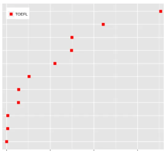
influ-ence of model parameters on TOEFL accuracy very well. Figure 1 displays the ranking of the evaluated parameters according to their importance in a fea-ture ablationsetting. TheR2 values in the plots
fer to the proportion of variance explained by the re-spective parameter together with all its interactions,
13*=p<0.05; ***=p<0.001; n.s. = not significant. 14Difference of means and Wilcoxon p-value on
Spear-man’s rhofor ratings datasets: RG65, −0.061***; WS353, −0.091***.
corresponding to the reduction in adjustedR2if this
parameter is left out. We do not rely on significance values for model selection because, given the large number of measurements, virtually all parameters have a highly significant effect.
criterion rel.index win.direction win.size context.dim corpus red.dim dim.skip transformation score metric 0 10 20 30 Partial R2 TOEFL
Figure 1: TOEFL, parameters and feature ablation Table 2 reports all parameter interactions for the TOEFL task that explain more than 0.5% of the total variance (i.e.R2≥0.5%), as well as the
correspond-ing degrees of freedom (df) andR2.
Interaction df R2 score:transf 18 7.42 metric:dim.skip 2 4.44 score:metric 6 1.77 metric:context.dim 4 0.98 win.size:transf 12 0.91 corpus:score 12 0.84 score:context.dim 24 0.64 metric:red.dim 4 0.63
Table 2: TOEFL task: interactions,R2
On the basis of their influence in determining model performance, we can identify three parame-ters that are crucial for the TOEFL task, and which will also turn out to be very influential in the other tasks at issue:distance metric,feature scoreand fea-ture transformation.
The best distance metriciscosine distance: this is one of the consistent findings of our evalua-tion study and it is in accordance with Bullinaria and Levy (2007) and, to a lesser extent, Kiela and Clark (2014).15 Score and transformation
al-ways have a fundamental impact on model
perfor-15In Kiela and Clark (2014),cosineis reported to be the best
● ● ● ● ● ● ● 55 60 65 70 75
frequency tf.idf MI Dice simple−ll t−score z−score transformation
●nonelog root sigmoid
Figure 2: TOEFL, score / transformation
● ● ● ● ● 55 60 65 70 75 1 2 4 8 16 transformation ●nonelog root sigmoid
Figure 3: TOEFL, window size / transformation
● ● ● ● 55 60 65 70 75 100 300 500 700 900 metric ● cosine manhattan
Figure 4: TOEFL, metric / n. of latent dim.
● ● ● 55 60 65 70 75 0 50 100 metric ● cosine manhattan
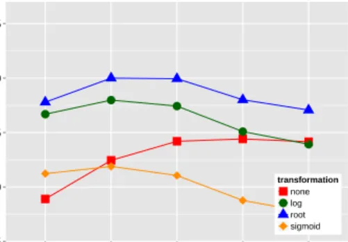
Figure 5: TOEFL, metric / n. of skipped dim. mance: these parameters affect the distributional
space independently of tasks and datasets. We will show that they are systematically involved in a strong interaction and that it is possible to iden-tify a score/transformation combination with robust performance across all tasks. The interaction be-tweenscoreandtransformationis displayed in fig-ure 2. The best results are achieved by association measures based on significance tests (simple-ll, t-score, z-score), followed byMI. This result is in line with previous studies (Bullinaria and Levy, 2012; Kiela and Clark, 2014), which found Pointwise MI or Positive MI to be the best feature scores. The best choice,simple-log likelihood, exhibits a strong vari-ation in performance across different transforma-tions. For all three significance measures, the best
feature transformationis consistently alogarithmic
transformation. Raw co-occurrencefrequency,tf.idf
andDice only perform well in combination with a squareroottransformation.
The best window size, as shown in figure 3, is a 2-word window for all evaluated transformations.
(a mean-adjusted version of cosine similarity). The latter, how-ever, turned out to be more robust across different corpora and weighting schemes.
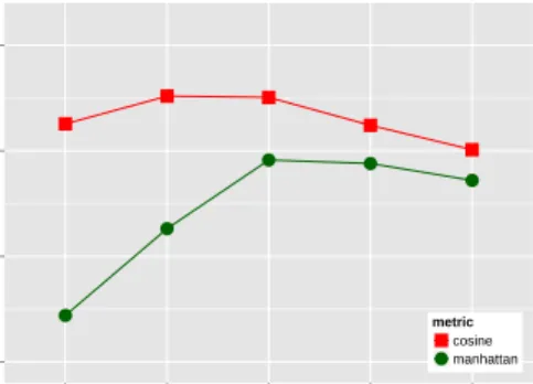
The SVD parameters (number of latent dimen-sions and number of skipped dimensions) play a significant role in determining model performance. They are particularly important for the TOEFL task, but we will see that their explanatory power is also quite strong in the other tasks. Interestingly, they show a tendency to participate in interactions with other parameters, but do not interact among them-selves. We display the interaction between metric
and number of latent dimensions in figure 4: the steep performance increase for both metrics shows that the widely-used choice of 300 latent dimen-sions (Landauer and Dumais, 1997) is suboptimal for the TOEFL task. The best value in our exper-iment is 900 latent dimensions, and additional di-mensions would probably lead to a further improve-ment. The interaction betweenmetricandnumber of skipped dimensionsis displayed in figure 5. While
manhattanperforms poorly no matter how many di-mensions are skipped, cosine is positively affected by skipping 100 and (to a lesser extent) 50 dimen-sions. The latter trend has already been discussed by Bullinaria and Levy (2012).
Inspection of the remaining interaction plots, not shown here for reasons of space, reveals that the best
DSM performance in the TOEFL task is achieved by selectingukwacascorpusand10000 original di-mensions. The index of distributional relatedness
has a very low explanatory power in the TOEFL task, withneighbor rankbeing the best choice (see plots 16 and 17 in section 5.4).
Given the minimal explanatory power of the di-rection of the context window and thecriterion for context selectionin all three tasks, we will not fur-ther consider these parameters in our analysis. We recommend to set them to an “unmarked” option:
undirectedandfrequency.
The best setting identified by inspecting all effects is shown in table 5, together with its performance and with the performance of the (over-trained) best model in this task. Parameters of the latter are re-ported in appendix A.
5.2 Ratings
Figure 6 displays the importance of the evaluated pa-rameters in the task of predicting similarity ratings. Parameters are ranked according to the average fea-ture ablationR2values across both datasets (adj.R2
of the full linear model: RG65: 86%; WS353: 90%).
● ● ● ● ● ● ● ● ● ● ● criterion win.direction context.dim dim.skip win.size red.dim rel.index metric transformation corpus score 0 10 20 30 Partial R2 ● RG65 WS353
Figure 6: Ratings, parameters and feature ablation Table 3 reports all interactions that explain more than 0.5% of the total variance in both datasets. For reasons of space, we only discuss the interactions and best parameter values on RG65; the correspond-ing plots for WS353 are shown only if there are sub-stantial differences.
As already noted for the TOEFL task,score and
transformationhave a large explanatory power and they are involved in a strong interaction showing the
Interaction df RG65 WS353 score:transf 18 10.28 8.66 metric:red.dim 4 2.18 1.42 score:metric 6 1.91 0.59 win.size:transf 12 1.43 1.01 corpus:metric 2 1.83 0.51 metric:context.dim 4 1.08 0.62 corpus:score 12 0.77 0.82 win.size:score 24 0.77 0.69 score:dim.skip 12 0.58 0.85
Table 3: Ratings datasets: interactions,R2
same tendencies and optimal values already iden-tified for TOEFL. For reasons of space, we do not elaborate on this interaction here.
The analysis of the main effects shows that for both datasets WaCkypedia is the best option as a source corpus, suggesting that this task bene-fits from a trade-off between quality and quan-tity (WaCkypedia being smaller and cleaner than ukWaC, but less balanced than the BNC).
Index of distributional relatedness plays a much more important role than for the TOEFL task, with
neighbor rank clearly outperforming distance (see figures 16 and 17 and the discussion in section 5.4 for more details).
The choice of the optimalwindow sizedepends on
transformation: on the RG65 dataset, figure 7 shows that for alogarithmictransformation – which we al-ready identified as the besttransformationin combi-nation with significance association measures – the highest performance is achieved with a4 word win-dow. The corresponding effect display for WS353 (figure 8) suggests that a further small improvement may be obtained with an8 word windowin this case. One possible explanation for this observation is the different composition of the WS353 dataset, which includes examples of semantic relatedness beyond attributional similarity. The 4 word window is a ro-bust choice across both datasets, though.
The number of latent dimensions is involved in a strong interaction with the distancemetric(figure 9). Best results are achieved with the cosine met-ricand at least300 latent dimensions, as well as 50
skipped dimensions. The interaction plot between
metricandnumber of original dimensionsin figure 10 shows that 50000 context dimensions are suffi-cient for good performance, and no further improve-ment can be expected from even higher-dimensional spaces.
● ● ● ● ● 0.45 0.50 0.55 0.60 0.65 0.70 0.75 1 2 4 8 16 transformation ●nonelog root sigmoid
Figure 7: RG65, window size / transformation
● ● ● ● ● 0.25 0.30 0.35 0.40 0.45 0.50 0.55 1 2 4 8 16 transformation ●nonelog root sigmoid
Figure 8: WS353, window size / transformation
● ● ● ● ● 0.45 0.50 0.55 0.60 0.65 0.70 0.75 100 300 500 700 900 metric ● cosine manhattan
Figure 9: RG65, metric / n. latent dim.
● ● ● ● ● 0.45 0.50 0.55 0.60 0.65 0.70 0.75 5000 10000 20000 50000 100000 metric ● cosine manhattan
Figure 10: RG65, metric / n. context dimensions Best settings for both datasets are summarized in
table 5. Refer to appendix A for best models.
5.3 Clustering
Figure 11 displays the importance of the evaluated parameters in the clustering task (adj.R2of the full
linear model: AP: 82%; BATTIG: 77%; ESSLLI: 58%; MITCHELL: 73%). Parameter ranking is de-termined by the average of the feature ablationR2
values over all four datasets.
● ● ● ● ● ● ● ● ● ● ● criterion win.direction rel.index context.dim dim.skip red.dim win.size metric corpus transformation score 0 10 20 30 Partial R2 ● AP BATTIG ESSLLI MITCHELL
Figure 11: Clustering, parameters and feat. ablation
Interaction df AP BATTIG ESSLLI MITCHELL score:transf 18 7.10 7.95 7.56 11.42 metric:red.dim 4 3.29 3.16 2.03 2.03 win.size:metric 4 2.22 1.26 2.97 2.72 win.size:transf 12 2.00 2.95 0.88 2.66 corpus:metric 2 1.42 2.91 2.79 1.11 metric:dim.skip 2 2.25 1.54 2.77 0.86 corpus:win.size 8 2.36 1.18 1.49 1.23 score:dim.skip 12 0.56 1.15 0.99 1.39 win.size:score 24 0.74 0.77 0.54 0.65
Table 4: Clustering task: interactions,R2
Table 4 reports all parameter interactions that ex-plain more than 0.5% of the total variance for each of the four datasets.
In the following discussion, we focus on the AP dataset, which is larger and thus more reliable than the other three datasets. We mention remarkable dif-ferences between the datasets in terms of best rameter values. For a full overview of the best pa-rameter setting for each dataset, see table 5.
As already discussed for TOEFL and the ratings task, we findscoreandtransformationat the top of the feature ablation ranking. Table 4 confirms that the two parameters are involved in a strong inter-action. The interaction plot (figure 12) shows the behavior we are already familiar with: significance
● ● ● ● ● ● ● 0.45 0.50 0.55 0.60
frequency tf.idf MI Dice simple−ll t−score z−score transformation
●nonelog root sigmoid
Figure 12: AP, score / transformation
● ● ● ● ● 0.45 0.50 0.55 0.60 1 2 4 8 16 metric ● cosine manhattan
Figure 13: AP, window size / metric
● ● ● ● ● 0.45 0.50 0.55 0.60 1 2 4 8 16 corpus ● bnc wacky ukwac
Figure 14: AP, corpus / window size
● ● ● 0.45 0.50 0.55 0.60 0 50 100 metric ● cosine manhattan
Figure 15: AP, metric / n. of skipped dim. measures (simple-ll, t-score and z-score) reach the
best performance in combination withlog transfor-mation: this combination is a robust choice also for the other datasets, with minor differences that can be observed in table 5 .
The interaction betweenwindow sizeandmetricis displayed in figure 13: best performance is achieved with a2 or 4 word windowin combination with co-sine distance. Results on the other datasets suggest a preference for the4 word window. This is confirmed by interaction plots withsource corpus(figure 14), which also reveal thatWaCkypediais again the best compromise between size and quality.
A very clear picture concerning the number of skipped dimensionsemerges from figure 15 and is the same for all datasets: skipping dimensions is not necessary to achieve good performance (even though skipping 50 dimensions turned out at least to be not detrimental for BATTIG and MITCHELL).
Further effect displays, not shown here for rea-sons of space, suggest that300 or 500 latent dimen-sions– with some variation across the datasets (cf. table 5) – and a medium-sized co-occurrence matrix (20000 or 50000 dimensions) are needed to achieve good performance.Neighbor rankis the best choice
as index of distributional relatedness (see section 5.4). See appendix A for best models.
5.4 Relatedness index
A novel contribution of our work is the systematic evaluation of a parameter that has received little at-tention in DSM research so far, and only in studies limited to a narrow choice of datasets (Lapesa and Evert, 2013; Lapesa et al., 2014; Zeller et al., 2014): theindex of distributional relatedness.
The aim of this section is to provide a full overview of the impact of this parameter in our ex-periments. Despite the main focus of the paper on the reduced setting, in this section we also show re-sults from the unreduced setting, for two reasons: first, since this parameter is relatively novel and evaluated here for the first time on standard tasks, we consider it necessary to provide a full picture concerning its behavior; second, relatedness index
turned out to be much more influential in the unre-duced setting than in the reunre-duced one.
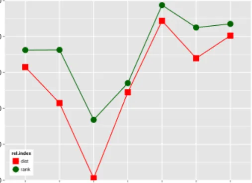
Figure 16 and 17 display the partial effect of relat-edness indexfor each dataset, in the unreduced and reduced setting respectively. To allow for a com-parison between the different measures of
perfor-● ● ● ● ● ● ● 30 40 50 60 70 80
TOEFL RG65 WS353 AP BATTIG MITCHELL ESSLLI
rel.index ●
dist rank
Figure 16: Unreduced Setting
● ● ● ● ● ● ● 30 40 50 60 70 80
TOEFL RG65 WS353 AP BATTIG MITCHELL ESSLLI
rel.index ●
dist rank
Figure 17: Reduced Setting mance, correlation and purity values have been
con-verted to percentages. The picture emerging from the two plots is very clear:neighbor rankis the best choice for both settings across all seven datasets. The degree of improvement over vector distance, however, shows considerable variation between dif-ferent datasets. The rating task benefits the most from the use of neighbor rank.
On the other hand, neighbor rank has very lit-tle effect for the TOEFL task in a reduced setting, where its high computational complexity is clearly not justified; the improvement on the AP clustering dataset is also fairly small. While the TOEFL result seems to contradict the substantial improvement of
neighbor rankfound by Lapesa and Evert (2013) for a multiple-choice task based on stimuli from prim-ing experiments, there were only two choices (con-sistent and incon(con-sistent prime) in this case rather than four. We do not rule out that a more refined use of the rank information (for example, different strategies for rank combinations) may produce bet-ter results on the TOEFL and AP datasets.
As discussed in section 3.2, we have not yet ex-plored the potential of neighbor rank in modeling directionality effects in semantic similarity. Unlike Lapesa and Evert (2013), who adopt four differ-ent indexes of distributional relatedness (vector dis-tance; forward rank, i.e., rank of the target in the neighbors of the prime; backward rank, i.e, rank of the prime in the neighbors of the target; average of backward and forward rank), we used only a single rank-based index (cf. section 3.2), mostly for rea-sons of computational complexity. We consider the results of this study more than encouraging, and ex-pect further improvements from a full exploration of directionality effects in the tasks at issue.
5.5 Best settings
We conclude the result overview by evaluating the best parameter combinations identified for each task and data set, showing how well our approach to model selection works in practice.
Table 5 summarizes the optimal parameter set-tings identified for each task and compares the per-formance of this model (B.set = best setting) with the over-trained best run in the experiment (B.run
= best run).16 In most cases, the result of our
ro-bust parameter optimization is close to the best run. The only exception is the ESSLLI dataset, which is smaller than the other datasets and particularly sus-ceptible to over-training (cf. the low R2 of the
gression analysis in section 5.3). Table 5 also re-ports the current state of the art for each task (SoA = state-of-the-art), taken from the ACL wiki17 where
available (TOEFL and similarity ratings), from Ba-roni and Lenci (2010) for the clustering tasks, and from more recent studies of which we are aware. Our results are comparable to the state of the art, even though the latter includes a much broader range of approaches than our window-based DSMs. In one case (BATTIG), our optimized model even improves on the best previous result.
A side-by-side inspection of the main effects and interaction plots for different data sets allowed us to identify parameter settings that are robustacross datasetsand evenacross tasks. Table 6 shows rec-ommended settings for each task (independent of the
16Abbreviations in the table: win = window size; c.dim=
number of context dimensions;tr= transformation;red.dim= number of latent dimensions;d.sk= number of skipped dimen-sions;r.ind= relatedness index; Parameter values:s-ll= simple-ll;t-sc= t-score;cos= cosine;man= manhattan.
Dataset corpus win c.dim score tr metric r.ind red.dim d.sk B.set B.run SoA Reference
TOEFL ukwac 2 10k s-ll log cos rank 900 100 92.5 98.7 100.0 Bullinaria and Levy (2012) RG65 wacky 4 50k s-ll log cos rank 500 50 0.87 0.89 0.86 Hassan and Mihalcea (2011)18
WS353 wacky 8 50k s-ll log cos rank 300 50 0.68 0.73 0.81 Halawi et al. (2012)19
AP wacky 4 20k s-ll log cos rank 300 0 0.69 0.76 0.79 Rotenh¨ausler and Sch¨utze (2009) BATTIG wacky 8 50k s-ll log cos rank 500 0 0.98 0.99 0.96 Baroni and Lenci (2010) ESSLLI wacky 2 20k t-sc log cos rank 300 0 0.77 0.98 0.91 Katrenko, ESSLLI workshop20
MITCHELL wacky 4 50k s-ll log cos rank 500 0 0.88 0.97 0.94 Bullinaria and Levy (2012) common for all datasets: window direction = undirected; criterion for context selection = frequency
Table 5: Best Settings particular dataset) and a more general setting that
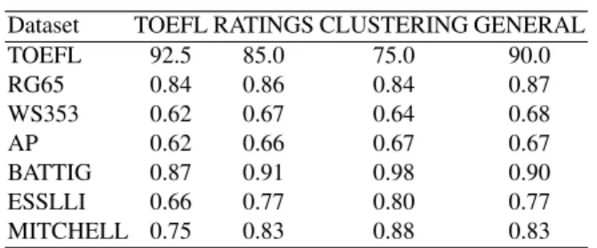
achieves good performance in all three tasks. Eval-uation results for these settings on each dataset are reported in table 7. In most cases, the general model is close to the performance of the task- and dataset-specific settings. Our robust evaluation methodol-ogy has enabled us to find a good trade-off between portability and performance.
Task corpus win c.dim score tr metric r.ind red.dim d.sk TOEFL ukwac 2 10k s-ll log cos rank 900 100 Rating wacky 4 50k s-ll log cos rank 300 50 Clustering wacky 4 50k s-ll log cos rank 500 0 General wacky 4 50k s-ll log cos rank 500 50
Table 6: General Best Settings
Dataset TOEFL RATINGS CLUSTERING GENERAL
TOEFL 92.5 85.0 75.0 90.0 RG65 0.84 0.86 0.84 0.87 WS353 0.62 0.67 0.64 0.68 AP 0.62 0.66 0.67 0.67 BATTIG 0.87 0.91 0.98 0.90 ESSLLI 0.66 0.77 0.80 0.77 MITCHELL 0.75 0.83 0.88 0.83
Table 7: General best Settings – Performance 6 Conclusion
In this paper, we reported the results of a large-scale evaluation of window-based Distributional Semantic Models, involving a wide range of parameters and tasks. Our model selection methodology is robust to overfitting and sensitive to parameter interactions.
18The ACL wiki lists the hybrid model of Yih and Qazvinian
(2012) as the best model on RG65 withρ=0.89, but does not specify its Pearson correlationr. In our comparison table, we show the best Pearson correlation, achieved by Hassan and Mi-halcea (2011), which is also the best corpus-based model.
19Halawi et al. (2012) report Spearman’sρ. Theρ values
for our best setting are: RG65: 0.85, WS353: 0.70; best setting for the ratings task: RG65: 0.82, WS353: 0.67; best general setting: RG65: 0.87, WS353: 0.70.
20http://wordspace.collocations.de/
It allowed us to identify parameter configurations that perform well across different datasets within the same task, and even across different tasks. We rec-ommend the setting highlighted in bold font in table 5 as a general-purpose DSM for future research. We believe that many applications of DSMs (e.g. vector compositon) will benefit from using such a param-eter combination that achieves robust performance in a variety of semantic tasks. Moreover, an exten-sive evaluation based on a robust methodology like the one presented here is the first necessary step for further comparisons of bag-of-words DSMs to dif-ferent techniques for modeling word meaning, such as neural embeddings (Mikolov et al., 2013). Let us now summarize our main findings.
• Our experiments show that a cluster of three pa-rameters, namely score, transformation and dis-tance metric, plays a consistently crucial role in determining DSM performance. These param-eters also show a homogeneous behavior across tasks and datasets with respect to best parameter values: simple-ll, log transformation andcosine distance. These tendencies confirm the results in Polajnar and Clark (2014) and Kiela and Clark (2014). In particular, the finding that sparse as-sociation measures (with negative values clamped to zero) achieve the best performance can be con-nected to the positive impact of context selection highlighted by Polajnar and Clark (2014): ongo-ing work targets a more specific analysis of their “thinning” effect on distributional vectors.
• Another group of parameters (corpus, window size, dimensionality reduction parameters) is also influential in all tasks, but shows more variation wrt. the best parameter values. Except for the TOEFL task, best results are obtained with the
WaCkypedia corpus, confirming the observation of Sridharan and Murphy (2012) that corpus
qual-ity compensates for size to some extent. Window size and dimensionality reduction show a more task-specific behavior, even though it is possible to find a good compromise in a4 word window, a reduced space of500 dimensionsandskipping of the first 50dimensions. The latter result confirms the findings of Bullinaria and Levy (2007; 2012) in their clustering experiments.
• Thenumber of context dimensionsturned out to be less crucial. While very high-dimensional spaces usually result in better performance, the increase beyond20000 or 50000 dimensionsis rarely suf-ficient to justify the increased processing cost.
• A novel contribution of our work is the systematic
evaluation of a parameter that has been given lit-tle attention in DSM research so far: theindex of distributional relatedness. Our results show that, even if the parameter is not among the most in-fluential ones,neighbor rank consistently outper-forms distance. Without SVD dimensionality re-duction, the difference is more pronounced: this result is particularly interesting for composition-ality tasks, where SVD has been reported to be detrimental (Baroni and Zamparelli, 2010). In such cases, the benefits of using neighbor rank
clearly outweigh the increased (but manageable) computational complexity.
Ongoing work focuses on the extension of the eval-uation setting to further parameters (e.g., new dis-tance metrics and association scores, Caron’s (2001) exponent p) and tasks (e.g., compositionality tasks, meaning in context), as well as the evaluation of dependency-based models. We are also working on a refined model selection methodology involv-ing a systematic analysis of three-way interactions and the exclusion of inferior parameter values (such as Manhattan distance, sigmoid transformation and Dice score), which may have a confounding effect on some of the effect displays.
Appendix A: Best models
This appendix reports the best runs for every dataset.21
21Some abbreviations are different from tables 5 and 6.
Pa-rameters:w= window;dir= direction;e= exclusion criterion for context selection; m= metric. Performance: acc= accu-racy;cor= correlation;pur= purity. Parameter values: dir= directed;undir= undirected;f= frequency;nz= non-zero.
corpus w dir e c.dim score tr m r.ind red.dim d.sk acc
ukwac 2 undir f 5000 MI none cos rank 900 100 98.75
ukwac 4 dir f 50000 t-score log cos rank 900 100 98.75 ukwac 4 undir f 50000 t-score root cos dist 900 100 98.75 ukwac 4 dir f 5000 simple-ll log cos dist 900 100 98.75
Table 8: TOEFL dataset – 23 models tied for best result (4 hand-picked examples shown)
corpus w dir e c.dim score tr m r.ind red.dim d.sk cor ukwac 16 undir nz 20000 MI none cos rank 700 100 0.89
ukwac 8 dir f 20000 MI none cos rank 700 100 0.89
wacky 4 dir nz 50000 simple-ll log cos rank 700 50 0.89 wacky 4 undir f 100000 z-score log cos rank 900 50 0.89
Table 9: Ratings, RG65 dataset – 19 models tied for best result (4 hand-picked examples shown)
corpus w dir e c.dim score tr m r.ind red.dim d.sk cor
wacky 16 dir f 5000 MI none man rank 900 50 0.73
wacky 16 undir f 5000 MI none man rank 900 50 0.72
wacky 16 undir f 5000 z-score log man rank 900 50 0.72 wacky 16 dir f 10000 z-score root man rank 900 50 0.72
Table 10: Ratings, WordSim353 dataset – best model (3 additional hand-picked models with sim-ilar performance are shown)
corpus w dir e c.dim score tr m r.ind red.dim d.sk pur ukwac 4 dir nz 10000 t-score log man rank 900 50 0.76 wacky 1 dir nz 10000 z-score log man rank 900 50 0.75 wacky 1 undir f 20000 simple-ll log man rank 900 50 0.75 wacky 2 dir f 100000 z-score log cos rank 500 0 0.75
Table 11: Clustering, Almuhareb-Poesio dataset – best model (plus 3 additional hand-picked models)
corpus w dir e c.dim score tr m r.ind red.dim d.sk pur ukwac 1 undir f 20000 Dice root man rank 300 100 0.99 ukwac 2 undir f 100000 freq log cos dist 300 50 0.99 wacky 16 undir f 50000 z-score log man dist 500 50 0.99 wacky 8 undir f 10000 Dice root man rank 500 0 0.99
Table 12: Clustering, Battig dataset – 1037 models tied for best result (4 hand-picked examples shown)
corpus w dir e c.dim score tr m r.ind red.dim d.sk pur wacky 16 dir nz 50000 z-score none man dist 900 0 0.98 ukwac 1 dir nz 100000 simple-ll log cos dist 100 50 0.95
ukwac 2 undir f 50000 tf.idf none man dist 700 0 0.95
wacky 8 undir f 100000 tf.idf root man rank 500 0 0.95
Table 13: Clustering, ESSLLI dataset – best model (plus 3 additional hand-picked models)
corpus w dir e c.dim score tr m r.ind red.dim d.sk pur bnc 2 undir nz 100000 simple-ll log cos rank 900 0 0.97 bnc 2 undir f 50000 simple-ll log cos rank 700 0 0.97 bnc 2 undir nz 50000 simple-ll log cos rank 900 0 0.97
Table 14: Clustering, Mitchell dataset – 3 models tied for best result
Acknowledgments
We are grateful to the editor and the anonymous re-viewers, whose comments helped us improve the paper. We would like to thank Sabine Schulte im Walde and the SemRel group at the IMS Stuttgart, the Corpus Linguistics group at the University of Erlangen-N¨urnberg and the Computational Linguis-tics group at the IKW Osnabr¨uck for their feedback on our work.
Gabriella Lapesa’s PhD research was funded by the DFG Collaborative Research Centre SFB 732 at IMS Stuttgart, where she conducted a large part of the work presented in this paper.
References
Abdulrahman Almuhareb. 2006. Attributes in Lexical Acquisition. Ph.D. thesis, University of Essex. Marco Baroni and Alessandro Lenci. 2010.
Distribu-tional memory: A general framework for corpus-based semantics.Computational Linguistics, 36(4):1–49. Marco Baroni and Roberto Zamparelli. 2010. Nouns
are vectors, adjectives are matrices: Representing adjective-noun constructions in semantic space. In
Proceedings of the 2010 Conference on Empiri-cal Methods in Natural Language Processing, pages 1183–1193, MIT, Massachusetts, USA.
Marco Baroni, Raffaella Bernardi, and Roberto Zampar-elli. 2014. Frege in space: A program for compo-sitional distributional semantics. Linguistic Issues in Language Technology (LiLT), 9(6):5–109.
John A. Bullinaria and Joseph P. Levy. 2007. Extract-ing semantic representations from word co-occurrence statistics: A computational study. Behavior Research Methods, 39:510–526.
John A. Bullinaria and Joseph P. Levy. 2012. Extract-ing semantic representations from word co-occurrence statistics: stop-lists, stemming and SVD. Behavior Research Methods, 44:890–907.
John A. Bullinaria and Joseph P. Levy. 2013. Limiting factors for mapping corpus-based semantic represen-tations to brain activity.PLoS ONE, 8(3):1–12. John Caron. 2001. Experiments with LSA scoring:
Optimal rank and basis. In Michael W. Berry, edi-tor,Computational Information Retrieval, pages 157– 169. Society for Industrial and Applied Mathematics, Philadelphia, PA, USA.
Stefan Evert. 2008. Corpora and collocations. In Anke L¨udeling and Merja Kyt¨o, editors,Corpus Linguistics. An International Handbook, chapter 58. Mouton de Gruyter, Berlin, New York.
Stefan Evert. 2014. Distributional semantics in R with the wordspace package. InProceedings of COLING 2014, the 25th International Conference on Compu-tational Linguistics: System Demonstrations, pages 110–114, Dublin, Ireland.
Lev Finkelstein, Evgeniy Gabrilovich, Yossi Matias, Ehud Rivlin, Zach Solan, Gadi Wolfman, and Eytan Ruppin. 2002. Placing search in context: The concept revisited. ACM Transactions on Information Systems, 20(1):116–131.
John Fox. 2003. Effect displays in R for generalised lin-ear models. Journal of Statistical Software, 8(15):1– 27.
Guy Halawi, Gideon Dror, Evgeniy Gabrilovich, and Yehuda Koren. 2012. Large-scale learning of word re-latedness with constraints. InProceedings of the 18th ACM SIGKDD international conference on Knowl-edge discovery and data mining, pages 1406–1414, New York, NY, USA.
Nathan Halko, Per-Gunnar Martinsson, and Joel A. Tropp. 2009. Finding structure with randomness: Stochastic algorithms for constructing approximate matrix decompositions. Technical Report 2009-05, ACM, California Institute of Technology.
Mary Hare, Michael Jones, Caroline Thomson, Sarah Kelly, and Ken McRae. 2009. Activating event knowl-edge. Cognition, 111(2):151–167.
Zelig Harris. 1954. Distributional structure. Word, 10(23):146–162.
Samer Hassan and Rada Mihalcea. 2011. Semantic relat-edness using salient semantic analysis. InProceedings of the Twenty-fifth AAAI Conference on Artificial Intel-ligence, pages 884 – 889, San Francisco, California. George Karypis. 2003. CLUTO: A clustering toolkit
(release 2.1.1). Technical Report 02-017, Minneapo-lis: University of Minnesota, Department of Computer Science.
Leonard Kaufman and Peter J. Rousseeuw. 1990. Find-ing groups in data: an introduction to cluster analysis. John Wiley and Sons.
Douwe Kiela and Stephen Clark. 2014. A systematic study of semantic vector space model parameters. In
Proceedings of EACL 2014, Workshop on Continu-ous Vector Space Models and their Compositionality (CVSC), pages 21–30, Gothenburg, Sweden.
Thomas K. Landauer and Susan T. Dumais. 1997. A so-lution to Plato’s problem: The latent semantic analysis theory of the acquisition, induction, and representation of knowledge. Psychological Review, 104:211–240. Gabriella Lapesa and Stefan Evert. 2013. Evaluating
neighbor rank and distance measures as predictors of semantic priming. InProceedings of the ACL Work-shop on Cognitive Modeling and Computational Lin-guistics (CMCL 2013), pages 66–74, Sofia, Bulgaria.
Gabriella Lapesa, Stefan Evert, and Sabine Schulte im Walde. 2014. Contrasting syntagmatic and paradig-matic relations: Insights from distributional semantic models. In Proceedings of the Third Joint Confer-ence on Lexical and Computational Semantics (*SEM 2014), pages 160–170, Dublin, Ireland.
Dekang Lin. 1998. Automatic retrieval and clustering of similar words. InProceedings of the 36th Annual Meeting of the Association for Computational Linguis-tics and 17th International Conference on Computa-tional Linguistics - Volume 2, pages 768–774, Mon-treal, Quebec, Canada.
Kevin Lund and Curt Burgess. 1996. Producing high-dimensional semantic spaces from lexical co-occurrence. Behavior Research Methods, Instrumen-tation and Computers, 28:203–208.
Tomas Mikolov, Kai Chen, Greg Corrado, and Jeffrey Dean. 2013. Efficient estimation of word represen-tations in vector space.CoRR.
Jeff Mitchell and Mirella Lapata. 2008. Vector-based models of semantic composition. In Proceedings of ACL-08: HLT, pages 236–244, Columbus, Ohio. Tom Mitchell, Svetlana V. Shinkareva, Andrew Carlson,
Kai-Min Chang, Vicente L. Malave, Robert A. Mason, and Marcel Adam Just. 2008. Predicting human brain activity associated with the meanings of nouns. Sci-ence, 320(5880):1191–1195.
Brian Murphy, Partha Talukdar, and Tom Mitchell. 2012. Selecting corpus-semantic models for neurolinguistic decoding. InProceedings of the First Joint Conference on Lexical and Computational Semantics - SemEval ’12, pages 114–123.
Sebastian Pad´o and Mirella Lapata. 2007. Dependency-based construction of semantic space models. Compu-tational Linguistics, 33(2):161–199.
Tamara Polajnar and Stephen Clark. 2014. Improving distributional semantic vectors through context selec-tion and normalisaselec-tion. In Proceedings of the 14th Conference of the European Chapter of the Asso-ciation for Computational Linguistics (EACL 2014), pages 230–238, Gothenburg, Sweden.
Klaus Rothenh¨ausler and Hinrich Sch¨utze. 2009. Un-supervised classification with dependency based word spaces. InProceedings of the EACL 2009 Workshop on GEMS: GEometical Models of Natural Language Semantics, pages 17–24, Athens, Greece.
Herbert Rubenstein and John B. Goodenough. 1965. Contextual correlates of synonymy. Communications of the ACM, 8(10):627—633.
Magnus Sahlgren. 2006. The Word-Space Model: Us-ing distributional analysis to represent syntagmatic and paradigmatic relations between words in high-dimensional vector spaces. Ph.D. thesis, University of Stockolm.
Gerard Salton, Andrew Wong, and ChungShu Yang. 1975. A vector space model for automatic indexing.
Communications of the ACM, 18(11):613–620. Hinrich Sch¨utze. 1998. Automatic word sense
discrimi-nation. Computational Linguistics, 27(1):97–123. Seshadri Sridharan and Brian Murphy. 2012.
Model-ing word meanModel-ing: Distributional semantics and the corpus quality-quantity trade-off. In Proceedings of the 3rd workshop on Cognitive Aspects of the Lexicon (CogAlex-III), pages 53–68, Mumbai, India.
Peter D. Turney and Patrick Pantel. 2010. From fre-quency to meaning: Vector space models of semantics.
Journal of Artificial Intelligence Research, 37:141– 188.
James Van Overschelde, Katherine Rawson, and John Dunlosky. 2004. Category norms: An updated and expanded version of the Battig and Montague (1969) norms. Journal of Memory and Language, 50:289– 335.
Wen-tau Yih and Vahed Qazvinian. 2012. Measur-ing word relatedness usMeasur-ing heterogeneous vector space models. In Proceedings of the 2012 Conference of the North American Chapter of the Association for Computational Linguistics: Human Language Tech-nologies (NAACL HLT ’12), pages 616–620, Montreal, Canada.
Britta Zeller, Sebastian Pad´o, and Jan ˇSnajder. 2014. To-wards semantic validation of a derivational lexicon. In
Proceedings of COLING 2014, the 25th International Conference on Computational Linguistics: Technical Papers, pages 1728–1739, Dublin, Ireland.