Efficient Parameterized Algorithms for Data Packing

Efficient Parameterized Algorithms for Data Packing

KRISHNENDU CHATTERJEE,

AMIR KAFSHDAR GOHARSHADY,

NASTARAN OKATI,

ANDREAS PAVLOGIANNIS,

There is a huge gap between the speeds of modern caches and main memories, and therefore cache misses account for a considerable loss of efficiency in programs. The predominant technique to address this issue has been Data Packing: data elements that are frequently accessed within time proximity are packed into the same cache block, thereby minimizing accesses to the main memory. We consider the algorithmic problem of Data Packing on a two-level memory system. Given a reference sequenceRof accesses to data elements, the task is to partition the elements into cache blocks such that the number of cache misses onRis minimized. The problem is notoriously difficult: it is NP-hard even when the cache has size 1, and is hard to approximate for any cache size larger than 4. Therefore, all existing techniques for Data Packing are based on heuristics and lack theoretical guarantees.

In this work, we present the first positive theoretical results for Data Packing, along with new and stronger negative results. We consider the problem under the lens of the underlyingaccess hypergraphs, which are hypergraphs of affinities between the data elements, where the order of an access hypergraph corresponds to the size of the affinity group. We study the problem parameterized by the treewidth of access hypergraphs, which is a standard notion in graph theory to measure the closeness of a graph to a tree. Our main results are as follows: we show there is a numberq∗depending on the cache parameters such that (a) if the access hypergraph of orderq∗has constant treewidth, then there is alinear-timealgorithm for Data Packing; (b) the Data Packing problem remains NP-hard even if the access hypergraph of orderq∗−1 has constant treewidth. Thus, we establish a fine-grained dichotomy depending on a single parameter, namely, the highest order among access hypegraphs that have constant treewidth; and establish the optimal valueq∗of this parameter. Finally, we present an experimental evaluation of a prototype implementation of our algorithm. Our results demonstrate that, in practice, access hypergraphs of many commonly-used algorithms have small treewidth. We compare our approach with several state-of-the-art heuristic-based algorithms and show that our algorithm leads to significantly fewer cache-misses.

Additional Key Words and Phrases: compilers, data packing, cache management, parameterized algorithms, data locality

1 INTRODUCTION

We consider the problem of Data Packing over a two-level memory system consisting of a small cache and a large main memory. Given a reference sequence of memory accesses to data elements, the goal is to organize the data elements into blocks in order to minimize cache misses. Intuitively, putting contemporaneously-accessed elements in the same block reduces the number of cache misses, but existing heuristic-based results do not present any theoretical guarantees. In this paper, we consider this problem from a theoretical perspective and establish its complexity by presenting exact algorithms and stronger hardness results. We also complement our theoretical results with an experimental evaluation.

Authors’ addresses: Krishnendu Chatterjee, IST Austria (Institute of Science and Technology Austria), Austria, krishnendu. [email protected]; Amir Kafshdar Goharshady, IST Austria (Institute of Science and Technology Austria), Austria, [email protected]; Nastaran Okati, Ferdowsi University of Mashhad, Iran, [email protected]; Andreas Pavlogiannis, École Polytechnique Fédérale de Lausanne (EPFL), Switzerland, [email protected].

2019. 2475-1421/2019/1-ART1 $15.00

Cache Management.Consider a memory system with an associative cache and a main memory. Data items are stored in the main memory and organized into sets of a small size, which are called

blocks (or pages). All data items have the same size and all blocks can hold the same number of data items. The cache has a small capacity and can hold a few blocks at any given time. Whenever a program needs to access a data element, its corresponding block must be present in the cache before the access can happen. Therefore, if the block is not already in the cache, it will be copied into the cache from the main memory, potentially by evicting another block. This copying process is called acache miss, and given the considerably slower speed of the main memory, cache misses are very

time-consuming and lead to significant overhead [Wulf and McKee 1995]. Therefore, the problem of

cache management, i.e., minimizing the number of cache misses, is of great importance in compilers

and operating systems. Cache management can naturally be divided in two parts [Calder et al.

1998]: (i) deciding on how to replace the blocks in the cache, i.e. which block to evict when the

cache is full and a miss occurs and (ii) deciding on the placement scheme of the data items inside

blocks. These problems are respectively calledPaging (or choosing a replacement policy)[Sleator

and Tarjan 1985] andData Packing[Lavaee 2016;Thabit 1982].

Paging (Replacement Policy).In paging, given a data placement scheme that divides the data

items into blocks and a so-calledreference sequenceof accesses to data elements, the problem is to

choose a block to be evicted each time a cache miss occurs. The goal is to do this in a way that

minimizes the total number of cache misses over the reference sequence [Panagiotou and Souza

2006]. An algorithm that chooses the block to be evicted is called areplacement policy. Common

replacement policies includeFIFO, which evicts the oldest block in the cache, andLRU, which evicts

the least recently used block [Borodin et al. 1995;Lavaee 2016]. Note that both FIFO and LRU can

also be applied in the online setting, i.e., when the algorithm does not know the entire sequence in advance and can only observe accesses as they are made. In the offline case, where the entire reference sequence is given in the beginning, the optimal replacement policy is to evict the block whose first use is furthest in the future [Borodin et al. 1995]. This is called theoptimal offline policy

(OOP). We primarily focus on LRU as the replacement policy, because it is the one that is most

commonly used in practice [Zhong et al. 2004].

Data Packing.The other aspect of cache management, which is the focus of this paper, is Data

Packing [Thabit 1982]. Consider a cache with a capacity ofmblocks, where each block can store

pdata items∗. Given a reference sequenceRof lengthN of accesses tondistinct data items and

a replacement policy, Data Packing asks for the optimal placement of data items into blocks in

order to minimize the number of cache misses. The parametersmandpare considered to be small

constants, and the complexity is studied wrtnandN which are large. Data Packing is an extremely

hard problem and is known to be hard to approximate within any non-trivial factor, i.e., any factor

significantly less thanN, unless P=NP [Lavaee 2016].

Relevance of Data Packing in Programming Languages.Data Packing is an important tech-nique for performance optimization during compilation and has been widely studied by the

pro-gramming languages community (See [Calder et al. 1998;Ding and Kennedy 1999;Lavaee 2016;

Petrank and Rawitz 2002;Zhang et al. 2006;Zhong et al. 2004]). The key relevance is two-fold:

• Limit studies:To test the performance of a compiler for data placement, various inputs can be generated as benchmarks, and the baseline comparison of the performance can be performed

against an optimal algorithm [Petrank and Rawitz 2002]. Hence, an optimal data packing

algorithm is necessary as the baseline.

∗

This necessarily means that there is a limit on the size of data items and a large item should be broken into smaller parts, each of which is considered a distinct data item.

• Profiling:Programs usually have similar memory-access behaviors over different inputs [

Pe-trank and Rawitz 2002]. Hence, an effective approximate approach for the online cache

management problem is to consider several representative inputs, then run an optimal offline algorithm for profiling, and then synthesize an answer to the online problem from optimal

offline solutions [Calder et al. 1998;Petrank and Rawitz 2002].

Previous theoretical results on data packing have all been negative (hardness) results.

Heuristics and Affinity.Given the hardness of cache management and Data Packing, the research in this area has been mostly focused on developing heuristics. The intuition behind many of these heuristics is to exploit the underlying affinities between data elements or blocks by trying to place elements that are commonly accessed together in the same block or evicting the block that is less

frequently accessed in conjunction with the rest of the blocks in the cache [Calder et al. 1998;

Ding and Kennedy 1999;Ding and Kandemir 2014;Han and Tseng 2006;Zhong et al. 2004]. Some

approaches, such as [Zhang et al. 2006], provide more sophisticated heuristics and construct a

hierarchy of affinities. However, none of the existing heuristics provide any theoretical guarantees.

Access Graphs.The concept of access graph [Borodin et al. 1995] has been introduced to model the affinities between data elements or blocks. An access graph is simply a graph in which there is a vertex corresponding to every data item and two vertices are connected by an edge if their respective items appear consecutively in the reference sequence. Access graphs might be weighted to model how many times every pair of elements have appeared consecutively. Similar structures

and extensions of access graphs to access hypergraphs have been introduced in [Lavaee 2016;

Thabit 1982] where they are called proximity (hyper)graphs. Moreover, most of the heuristic-based

approaches also consider variants of the notion of access graphs.

Cache Misses vs Cache Hits.We consider the Data Packing problem, which asks to minimize the cache misses. Its natural dual problem is to maximize cache hits. While the two problems are equivalent in case of exact algorithms, an approximation algorithm for maximum cache hits does

not necessarily lead to an approximation for minimum cache misses [Lavaee 2016]. For example, if in

an access sequence of lengthNwe haveN−

√

Ncache hits and

√

Ncache misses, an approximation

ofN−

√

Nhits can lead to an arbitrarily bad approximation of

√

Ncache misses. In practice, cache

misses occur much less frequently than cache hits, but contribute significantly to the overhead. Thus, approximation of cache misses is more important than approximation of cache hits, and the Data Packing problem is defined in terms of cache misses.

Previous Results on Cache Management.To the best of our knowledge, all theoretical results on minimizing cache misses are negative or hardness results. We summarize some of the main

results in this area. Given a reference sequenceRof lengthN and a cache with a capacity ofm

blocks, the following results have been shown:

(i) In [Petrank and Rawitz 2002], the authors considered the problem of Cache-conscious Data

Placement, which is a somewhat different formulation of cache-miss minimization and is intuitively similar and related to Data Packing. In Cache-conscious Data Placement, a cache

consists ofmlines, each capable of holding up topdata items at any given time. The problem

is to assign each data itemdto a cache linel_d. When the program wants to access the data

itemd, it should be present in cache linel_d, otherwise a cache miss occurs anddis copied to

ld, potentially by evicting another data item froml_d. Given an eviction strategy, the goal is to

assign data items to cache lines in a manner that minimizes cache misses. In [Petrank and

Rawitz 2002] it was shown that the problem is NP-hard and unless P=NP, it cannot even be

(ii) In the same paper, it was shown that any algorithm that does not process the entire sequence, but instead relies on pairwise affinity information on data items, such as the access graph,

cannot find a solution within a factor ofm−3 from the optimal, even with unbounded time.

(iii) In [Lavaee 2016], the author showed that Data Packing is NP-hard for any cache size and hard

to approximate within a factor ofO(N1−ϵ)unless P=NP.

Given these hardness results, Data Packing is usually handled by heuristic-based algorithms that do not provide any theoretical guarantee. The only positive theoretical result deals with approximating maximum cache hits:

(iv) In [Lavaee 2016] it was established that the dual problem of Data Packing with the goal of

maximizing cache hits, instead of minimizing cache misses, is approximable within a constant factor. However, this does not approximate the optimal number of cache misses.

Exploiting Structural Properties.Data Packing is a notoriously difficult computational problem. In dealing with this problem, a direction that has not been pursued is to exploit structural properties of the access graphs. In many cases, structural properties of graphs help in obtaining efficient parametrized algorithms for computationally-hard problems. Specifically, a well-studied structural property in graph theory, which is frequently applied to computationally-hard graph problems, is

the notion oftreewidth. We present this notion below.

Treewidth.Treewidth [Robertson and Seymour 1984] is a well-known and extensively-studied parameter in graph theory. The treewidth of a graph is a measure of how tree-like the graph is. Specifically, trees and forests are the only graphs with a treewidth of 1. The importance of treewidth in algorithm design stems from the fact that many NP-hard graph problems (e.g., Vertex Cover and Hamiltonian Cycle) can be solved in polynomial time if the input graphs have constant treewidth

and moreover, many other graph problems can be solved in a lower complexity [Abboud et al.

2016;Bodlaender 1997;Chatterjee et al. 2018;Cygan et al. 2015;Fomin et al. 2017;Robertson and

Seymour 1986]. The formal definition of treewidth is presented in the next section.

Treewidth in Program Analysis.Many important families of graphs that arise commonly in algorithm design are shown to have constant treewidth, e.g., series-parallel and outer-planar

graphs [Bodlaender 1998]. Perhaps the most important example in program analysis is that the

control-flow graphs of structured goto-free programs in many languages such as Pascal and C++

have constant treewidth [Thorup 1998]. The same result was also shown experimentally for most

Java programs [Gustedt et al. 2002]. This led to algorithmic advances in verification and program

analysis [Chatterjee et al. 2015a]. Moreover, treewidth has also been exploited to obtain faster

algorithms for static analysis of recursive state machines [Chatterjee et al. 2015b] and concurrent

systems [Chatterjee et al. 2016,2017].

Treewidth in Data Packing.In this work we show that Data Packing can be reduced to a graph problem. In many cases when a graph arises from a structured process, the treewidth of the graph

is not very large [Bodlaender 1998]. For Data Packing, the access graphs arise from structured

program accessing data from a well-defined data structure. Thus, it is natural to study the problem of Data Packing in terms of the treewidth property of the arising graphs, as we do in this work. Our Contributions.Our contributions include (a) polynomial algorithms for Data Packing in constant treewidth access (hyper)graphs, (b) stronger hardness results, and (c) experimental results demonstrating that our approach leads to considerably fewer cache misses in comparison with

previously-known heuristic-based approaches. Concretely, consider that the cache has sizem, every

block can holdpdata items and the reference sequence is of lengthN withndistinct items. We

consider the access hypergraph of orderq, where each vertex of the graph is a data item, and an

edge connects a set ofqdistinct data items if they appear contiguously in the reference sequence.

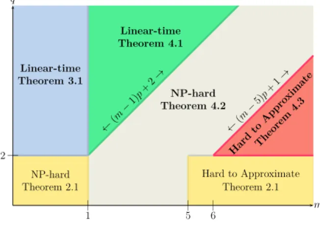
Hard toAppro ximate Theorem 4.3 ←( m− 5)p +1 → NP-hard Theorem 4.2 ←( m− 1)p +2 → Linear-time Theorem 4.1 Hard to Approximate Theorem 2.1 NP-hard Theorem 2.1 Linear-time Theorem 3.1 | 1 5| 6| | 2 m q

Fig. 1. The complexity of Data Packing forp≥3. Heremis the cache size andqis the highest order for which

the access hypergraph has constant treewidth. For a formal definition of order see Section2.1. Theorem2.1

was established in [Lavaee 2016]. The rest of the picture is filled by this paper. Our results are shown in bold.

access (hyper)graph and we study whether the constant treewidth property can be exploited for

polynomial-time algorithms. Our main results, assuming constantmandp, are as follows:

(1)Results on Access Graphs.We first considerq=2. Note that order-2 access hypergraphs are basically access graphs. We establish the following results:

• Linear-time algorithm.We present a linear-time algorithm for Data Packing when the

access graph is of constant treewidth andm=1 (Theorem3.1).

• Hardness of the exact problem.The Data Packing problem remains NP-hard form≥2 and

p ≥3 even if the underlying access graph is a tree (which has treewidth 1) (Theorem3.2).

• Hardness of approximation.Unless P=NP, for anym≥6,p ≥2 and any constantϵ >0,

the Data Packing problem is hard to approximate within a factor ofO(N1−ϵ)even if the

underlying access graph is a tree (Theorem3.2).

(2)Results on Access Hypergraphs.We define access hypergraphs of higher orders and consider

their treewidth. Letq∗=(m−1)p+2. Note thatq∗depends only on the cache parameters, and

not onnorN. We consider the access hypergraph of orderq∗. Intuitively, every edge of this

access hypergraph contains all the necessary historical cache data for determining whether a miss occurs at a corresponding memory access. Formally, we establish the following results:

• Linear-time algorithm.We present a linear-time algorithm for Data Packing when the

access hypergraph of orderq∗has constant treewidth (Theorem4.1).

• Hardness of the exact problem.Form≥2 andp ≥3, the Data Packing problem remains

NP-hard even if the access hypergraph of orderq∗−1 has constant treewidth (Theorem4.2).

• Hardness of approximation.Unless P=NP, form≥6 andp ≥2 and any constantϵ >0, the

Data Packing problem is hard to approximate within a factor ofO(N1−ϵ)even if the access

hypergraph of orderq∗−4p−1 has constant treewidth (Theorem4.3).

Note that while constant treewidth has been exploited to obtain polynomial-time algorithms for NP-complete graph problems such as Vertex Cover and Hamiltonian Cycle, we show that for Data Packing the constant treewidth property does not always help, and the problem

remains hard even when the access hypergraph of orderq∗−1 has constant treewidth.

Our hardness result and linear-time algorithm present a sharp boundary (or fine-grained dichotomy) that shows when the treewidth can be exploited. Concretely, the hardness of

the Data Packing problem can be captured by a single parameter, namely, the highest order

amongst access hypergraphs that have constant treewidth. We establish the optimal valueq∗

of this parameter which is the necessary and sufficient condition for existence of efficient parameterized algorithms that exploit treewidth.

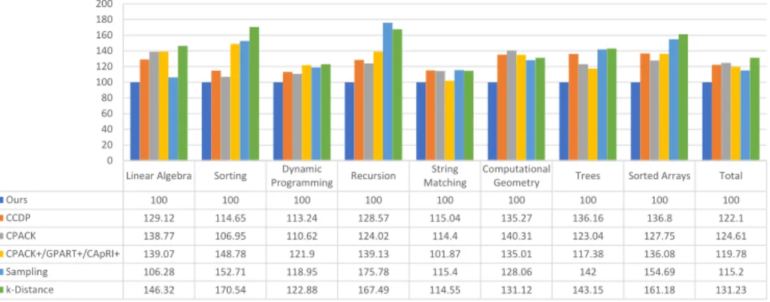
(3)Experimental results.We present an experimental evaluation of a prototype implementation of our algorithm on a variety of benchmarks from linear algebra, sorting algorithms, dy-namic programming, recursive algorithms, string matching, computational geometry and algorithms on tree data-structures. Our results show that the access hypergraphs of most of the benchmarks have small treewidth. We compare our approach with several state-of-the-art heuristic-based algorithms. The experimental results show that on average our optimal algorithms obtain 15-30% imporvement over the previous heuristic-based approaches. Novelty and Significance.In this paper, we define a novel and rich structural property of programs, i.e. access hypergraphs and their treewidth, and show that it can be exploited to obtain faster algorithms for Data Packing. We present the first positive theoretical results for Data Packing, i.e.,

for cache-miss minimization. We also enrich the complexity landscape as shown in Figure1. Only

the results of Theorem2.1were known before, and all other results (which are shown in bold) are

established in the present work.

2 PRELIMINARIES 2.1 Data Packing

In this section, we define the problem of data packing and fix our notation. We also present several

previously-known results. The problem was first studied in [Thabit 1982]. Here, we present an

adaptation of its definition as formalized in [Lavaee 2016].

Notation.We use_Zto denote the set of integers and_Nto denote the set of positive integers. Let

G =(V,E)be a (hyper)graph, andX ⊆V, then we denote byG[X], the induced subgraph ofG

overX, i.e.G[X]=(X,{e∈E|e ⊆X}). Given two (hyper)graphsG1=(V1,E1)andG2=(V2,E2),

we define their union and intersection in the natural way, i.e.G1∪G2 =(V1∪V2,E1∪E2)and

G1∩G2=(V1∩V2,E1∩E2). IfF is a family of sets, we write∪F (resp.∩F) to denote∪A∈ FA (resp.

∩_A∈ FA). Given two functions f,д :A→_Z, equality and summation are defined in a pointwise

manner, i.e.f ≡д ⇔ ∀a ∈A; f(a)=д(a)and for anya ∈A, we have(f +д)(a)= f(a)+д(a).

Given a functionf :A→Band a subsetA′⊆A, we usef_|A′to denote the restriction off toA′.

This restriction is a function of the formf_|A′:A′→Bthat agrees withf on every point inA′. For

a setX, we writeP(X)to denote the power set ofX, i.e., the set of all subsets ofX.

Data Placement Schemes.Given a setDof sizenof data items and a positive integerp, a data

placement schemeσis a partitioning ofDinto blocks of size at mostp. We callpthepacking factor.

It is often useful to think ofσas an equivalence relation onDwhose equivalence classes are the

blocks. Hence, following the usual notation, we writexσyto denote thatxandyare in the same

block,[x]_σ to denote the block ofσthat contains the data elementxandD/σ to denote the set of

blocks or equivalence classes ofσ.

Replacement Policies.Given a setDofndata items, a cache of sizem, a data placement scheme

σ, and a sequenceR ∈DN of accesses to data items, a replacement policy is a function that decides

which block must be evicted from the cache at each time. Formally, a replacement policy is a functionπ:{0,1,2, . . . ,N} →P(D/σ)that assigns to each time pointi, the set of blocks that are

present in the cache right after the accessR[i]. Any such policy must satisfy the following:

• π(0)=∅, i.e. the cache must be empty at the beginning;

• For all 1≤i≤N,|π(i) \π(i−1)| ≤1 and|π(i−1) \π(i)| ≤1, i.e. at most one block can be added to the cache and at most one block can be evicted at each step;

• For all 1≤i ≤N,R[i] ∈ ∪π(i), i.e. the block containing an accessR[i]must be in the cache right after that access.

Remark 2.1. Note that the replacement policy only matters when the cache has a size of at least2.

When the cache has unit size, there is always a unique choice for the block that must be evicted.

Cache Misses.Given a data placement schemeσand a replacement policyπas above, the number

of cache misses caused byσ andπoverRis defined as the number of times a new block is loaded

into the cache. Formally, misses(σ,π)=| {i |1≤i ≤N,π(i) \π(i−1)_,∅} |.

The LRU Policy.Due to its popularity, we assume throughout this paper that the replacement policy is LRU, i.e. the Least-Recently-Used block is always evicted from the cache. However, most of our results carry over to First-In-First-Out (FIFO) and the Optimal Offline Policy (OOP), as well. Recall that FIFO evicts the oldest block in the cache and OOP evicts the block that is going to be used furthest in the future.

The Data Packing Optimization Problem.Consider a memory subsystem that consists ofn

distinct data elements and a fully-associative cache with a capacity ofmblocks and a packing factor

ofp. Given a sequenceRof lengthN of references to data elements, the Data Packing problem

asks for a data placement schemeσthat minimizes the number of cache misses incurred by the

reference sequenceR, using LRU as the replacement policy. We denote an instance of the Data

Packing problem byI =(n,m,p,R).

Parameters.In the sequel, we consider the parametersmandpto be small constants and try to

find polynomial algorithms in terms ofN andn.

We now define the concepts of access graph and access hypergraph. Various similar notions have been defined in the past, and are sometimes called affinity graphs or proximity graphs. These hypergraphs will later serve as a basis for reducing the Data Packing problem to a graph problem. Access Graph.Given a sequenceR of length N of accesses to data elements from a setD of

sizen, the access graph ofRis a simple graphG_R=(V,E)in whichV consists ofnvertices, each

corresponding to one of the data elements inD, and there is an edge between two distinct vertices iff

their corresponding data elements appear consecutively somewhere inR. More formally,{u,v} ∈E

iffu_,vand there exists an indexi, such that{R[i],R[i+1]}={u,v}.

Intuitively, one can think of the graphG_Ras the structure on data elements that is respected by

the access sequenceR, in the sense thatRcan only go from a vertex inG_Rto one of its neighbors.

Moreover,G_Ris the sparsest graph over whichRis a (non-simple) path.

Example 2.1. Consider the access sequenceR=<a,b,c,a,b,b,d,b,d,e,c,b,f >. There are 6 data

elements in this sequence and its access graphGRis shown in Figure2. Note thatRis a path on this

graph and every edge appears somewhere alongR, hence no subgraph ofGRhas the same property.

a b c d e f

We now extend the concept of access graphs to higher order affinity relations between data items, resulting in access hypergraphs.

Hypergraphs and Ordered Hypergraphs.A hypergraphG =(V,E)consists of a setVof vertices

and a multisetEof hyperedges. Each hyperedgee∈Eis in turn asubsetof the vertices ofG. An

ordered hypergraphG=(V,E)consists of a setV of vertices and a setEof ordered hyperedges.

Each ordered hyperedgee∈Eis asequenceof distinct vertices ofG, i.e. a hyperedge together with

an order on its vertices. Intuitively, hypergraphs are natural extensions of graphs, where each edge

can connect more than two vertices. Given a hypergraphG, its primal graphGpis a graph on

the same setV of vertices, where two verticesuandvare connected by an edge iff there exists a

hyperedgee ∈Econtaining bothuandv. We shall simply refer to hypergraphs and hyperedges as

graphs and edges when there is no fear of confusion.

Access Hypergraph.Given a natural numberqand an access sequenceR as above, the access

hypergraphGq

R=(V,E)is a hypergraph defined as follows:

• There arenvertices inV, each corresponding to one data element;

• For each data accessR[i], there is a corresponding hyperedgee_i inE. The hyperedgee_i

consists ofR[i]and theq−1 distinct data elements that are accessed right beforeR[i]. If

there are less thanq−1 such elements,e_i will include all of them. Concretely,e_i is defined as

follows:e_i :={R[j] |j≤i∧ |{R[j],R[j+1], . . . ,R[i]}| ≤q}.

We callqtheorderof the access hypergraph. It is easy to verify that removing repeated edges from

the access hypergraphG2_Rleads to the access graphG_R.

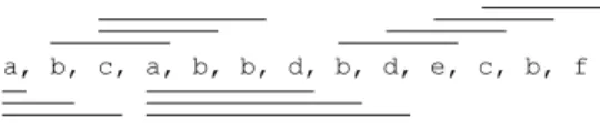
Example 2.2. Consider the access sequenceR =<a,b,c,a,b,b,d,b,d,e,c,b,f >. Lettingq =3,

the corresponding access hypergraphG3

Rof order3consists of the following hyperedges (sometimes

there are multiple copies of the same hyperedge, as shown below. We consider these to be distinct hyperedges):{a},{a,b},{a,b,c} ×4,{a,b,d} ×3,{b,d,e},{c,d,e},{b,c,e},{b,c,f}.Figure3shows

the segments of the sequence that correspond to edges inG3 R.

a, b, c, a, b, b, d, b, d, e, c, b, f

Fig. 3. Segments ofRcorresponding to edges in the hypergraphG3

R

Ordered Access Hypergraphs.Given an access sequenceRas above, the ordered access hyper-graphGˆq

R is defined similarly toGq

R, except that each hyperedge is ordered in the natural way,

i.e. in the order of appearance of its corresponding data elements inR. Formally, for every access

R[i], there is a corresponding ordered hyperedgee_i inGˆq_R. The ordered hyperedgee_i is a sequence

< v1,v2, . . . ,vl >of vertices ofGˆ q

R such thatv_l = R[i],v_l−1 is the first distinct data element

accessed beforeR[i],v_l−2is the second distinct element, etc. Moreover,lis the maximum between

qand the number of distinct elements accessed up untilR[i].

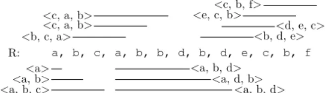
Example 2.3. Consider the access sequenceR =< a,b,c,a,b,b,d,b,d,e,c,b,f >. The access

hypergraphG3

Rwas shown in Example2.2. We now construct the ordered hyperedges ofGˆR3. Intuitively,

we start from any accessR[i]inRand go back until we see3different data elements. These data

elements will form the ordered hyperedgeei corresponding toR[i]. This is illustrated in Figure4. Note that the elements in an ordered hyperedgeei are ordered by their last access time before or atR[i], e.g. see the hyeperedge<a,d,b>in Figure4.

a, b, c, a, b, b, d, b, d, e, c, b, f <a> <a, b> <a, b, c> <b, c, a><c, a, b> <c, a, b> <a, b, d> <a, d, b> <a, b, d> <b, d, e><d, e, c> <e, c, b><c, b, f> R:

Fig. 4. Ordered Hyperedges ofGand the segments inRto which they correspond

2.2 Tree Decompositions and Treewidth

In parameterized complexity, treewidth is one of the most widely-used parameters for graph problems. It is a measure of how “tree-like” a given graph is. In this section, we provide a quick

overview of tree decompositions and treewidth. For an in-depth treatment see [Cygan et al. 2015].

Tree Decomposition. Given a (hyper)graphG = (V,E), a tree decomposition ofG is a pair

(T,{X_t |t ∈T})whereT is a tree and each nodetofT is associated with a subsetX_t ⊆V of

vertices ofG, such that the following conditions are met:

(i) Every vertex appears in someX_t, i.e.∪_t∈TX_t =V;

(ii) Every (hyper)edge appears in someX_t, i.e.∀e∈E ∃X_t e⊆X_t;

(iii) For every vertexv ∈V, the setT_v={t ∈T|v∈X_t}of all nodes of the treeT that containvin

their correspondingX_t, forms a connected subtree ofT.

It is evident from the definition that(T,{X_t})is a tree decomposition of a hypergraphGiff it is

a tree decomposition of its primal graphGp. To avoid confusion, we reserve the word “vertex” for

vertices ofGand use the word “node” for vertices ofT. Moreover, we call eachX_t a “bag”.

Treewidth.The width of a tree decomposition (T,{X_t})is the size of its largest bag minus 1,

i.e. min_t∈T |X_t|- 1. The treewidth of a graphGis the smallest width among all tree decompositions

ofGand is denotedtw(G).

Example 2.4. Figure5shows the graphG_R(as in Figure2) and a tree decomposition ofG_R. This tree

decomposition has a width of 2 and is an optimal tree decomposition. Hence, the treewidth ofGRis 2. a b c d e f {a,b,c} {b,c,d} {b,f} {c,d,e}

Fig. 5. A graphGR(left) and one of its optimal tree decompositions(T,{X_t})(right).

To simplify the algorithms that exploit tree decompositions, we now define the notions of labeling and nice tree decomposition.

Nice Tree Decompositions.A nice tree decomposition [Cygan et al. 2015] of a (hyper)graphGis

a tree decomposition(T,{X_t})in which a specific node is designated as the root and every node

t ∈T is “labeled” by a subgraphG_t ofG, such that the following rules are obeyed:

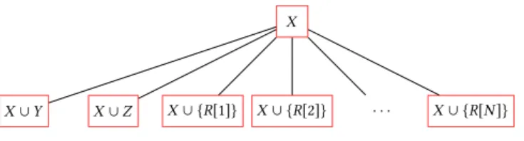
(1) Iftis a leaf inT, thenX_t =∅andG_t =(∅,∅).

(2) Otherwise,tsatisfies one of the following cases:

• Introduce Vertex Node.The nodethas a single childt1andXt =Xt1∪ {v}for some vertex v<Xt1. In this case, we say thattintroducesv. Moreover,Gt =Gt1∪ {v}, i.e.Gtis defined

as the graph resulting from addingvas an isolated vertex toG_t

1.

• Introduce Edge Node.Similar to the previous case,thas a single childt1. This time,Xt =Xt1,

butG_tis defined as the graph resulting from adding a new edgeetoG_t

1. All vertices ofe

must be present inX_t. We say thattintroducese.

• Forget Vertex Node.The nodethas a single childt1andXt =Xt1\ {v}for some vertex v ∈Xt1. We say thattforgetsv. Moreover,Gt =Gt1.

(3) Each edge is introduced exactly once.

Intuitively, the label graphG_tis the subgraph ofGconsisting of all the vertices and edges that are

introduced in the subtree ofT rooted att.

Remark 2.2. Note that in our (ordered) hypergraphs in this paper, we might have multiple copies

of the same (ordered) hyperedge. We treat these as distinct edges and require that each of them be introduced separately in nice tree decompositions.

Remark 2.3. The notion of label graphsG_t is solely defined for theoretical purposes and used in our

proofs of correctness. In practice, our implementation avoids the overhead of constructingGt’s.

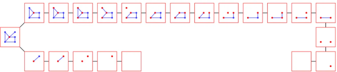
Example 2.5. Figure6shows a nice tree decomposition of the graphGof Figure2. In each nodetof

the tree, its label subgraphGt is illustrated and the vertices of the bagXt are shown in red. Intuitively, a nice tree decomposition constructs the graph in small increments and the bagXtcontains the vertices

that can participate in the incremental change.

Fig. 6. A nice tree decomposition of the graph in Figure2. The leftmost node is the root. The graphGtis

illustrated in each nodet. The vertices of the bagsXt are shown in red.

2.3 Existing Results

We now formally present known results regarding Data Packing and Tree Decompositions that will be used in the sequel.

The Hardness of Data Packing.Note that we are considering the problem of minimizing cache misses, not that of maximizing cache hits. While the two problems are equivalent in terms of exact algorithms, approximating the minimal number of cache misses is much harder than approximating the maximal number of cache hits. The latter problem admits a polynomial-time constant-factor

approximation [Lavaee 2016]. In contrast, the following theorem shows that the former problem is

hard to even approximate.

Theorem 2.1 ([Lavaee 2016]). Assuming either LRU, FIFO or OOP as the replacement policy, we

have the following hardness results:

• For anymand anyp≥3, Data Packing is NP-hard.

• Unless P=NP, for anym≥5,p ≥2and any constantϵ >0, there is no polynomial algorithm

that can approximate the Data Packing problem within a factor ofO(N1−ϵ

We now turn to tree decompositions. What makes tree decompositions a very useful tool is the fact that one can perform bottom-up dynamic programming on them in a manner similar to trees. This is due to an property of tree decompositions, called the separation lemma.

Separators.Given a (hyper)graphG=(V,E), and two sets of verticesA,B ⊆V, we say that the

pair(A,B)is a separation ofGifA∪B=V and no (hyper)edge inEcontains vertices of bothA\B

andB\A. We callA∩Bthe separator corresponding to the separation(A,B)and the order of the

separation(A,B)is the size of its separator|A∩B|.

Lemma 2.1 (Separation Lemma, [Bodlaender 1988;Cygan et al. 2015]). Let(T,{X_t})be a tree

decomposition ofG, whereGis a graph or a hypergraph, and let{a,b}be an edge ofT. By removing the edge{a,b},T breaks into two connected componentsTaandTb, respectively containingaandb.

LetA=Ð

t∈TaXtandB= Ð

t∈TbXt. Then(A,B)is a separation ofGwith separatorXa∩Xb.

In our algorithms in the rest of this paper, we assume that whenever a (hyper)graphG of

constant treewidth appears as an input to an algorithm, the input also contains an optimal nice

tree decomposition(T,{X_t})ofG. This is justified by the following two lemmas that show one can

obtain(T,{X_t})fromGin linear time.

Lemma 2.2 ([Bodlaender 1996] ). There is an algorithm that given a (hyper)graphG=(V,E)

and a constantk, decides in linear time whetherGhas treewidth at mostkand if so, produces a tree decomposition ofGwith optimal width andO(k· |V|)nodes.

Lemma 2.3 ([Cygan et al. 2015]). There is a linear-time algorithm that given a graphG=(V,E)

and a tree decomposition (T,{Xt}) ofG of widthk with O(k · |V|)nodes, produces a nicetree

decomposition(T′,{Xt′})ofGwith the same widthkandO(k· |V|)nodes. This algorithm can also be applied ifGis a hypergraph, in which case the output tree decomposition(T′,{Xt′})will have widthk andO(k· |V|+|E|)nodes.

3 DATA PACKING ON CONSTANT-TREEWIDTH ACCESS GRAPHS

We now consider the problem of Data Packing when parameterized by the treewidth of the

underlying access graph. In Section3.1, we provide a linear-time algorithm whenm=1 and the

access graph has constant treewidth. Note that this problem is NP-hard for general access graphs,

as demonstrated by Theorem2.1. Then, in Section3.2we show that form≥2 the problem remains

NP-hard and hard-to-approximate even when the access graph is a tree, i.e. has treewidth 1.

3.1 Algorithm form=1and Constant-treewidth Access Graph

We are given a Data Packing instanceI =(n,1,p,R), its access graphG_Rand a nice tree

decomposi-tion(T,X_t)of the access graph with widthkandO(n·k)nodes. We first reduce the problem of

Data Packing to a graph problem overG_Rand then provide a linear-time fixed-parameter algorithm

for solving the graph problem. We start by defining the minimum-weightp-partitioning problem.

p-partitionings.Given an integerp > 0 and a graphG = (V,E), ap-partitioning ofG is a

partitioningψof the setV of vertices such that each partition set has a size of at mostp. In other

words, ap-partitioning ofG is a data placement scheme where the vertices ofG are the data

elements andpis the packing factor.

Cross Edges.Given ap-partitioningψ of the graphG=(V,E), an edgee ={u,v} ∈Eis called a cross edge if its two endpoints are in different partition sets, i.e. if[u]_{ψ ,}[v]_ψ.

Minimum-weightp-partitioning.Given a simple graphG=(V,E), a weight functionw :E→_N

and a positive integerp, the minimum-weightp-partitioning problem asks for ap-partitioning ofG

a b c d e f 2 1 3 1 1 2 1

Fig. 7. An optimal2-partitioning

Reduction of Data Packing to Minimum-weightp-partitioning.We now reduce the Data

Packing problem to minimum-weightp-partitioning. Given an instanceI =(n,1,p,R)of Data

Packing, we consider the access graphG_R=(V,E)and define the weight functionw_R:E→_Nas

wR({u,v}):=|{i| {R[i],R[i+1]}={u,v}}|.Informally, the weight of an edge is the number of

times its two endpoints have appeared consecutively inR. The reduction is now complete.

Lemma 3.1. The optimal number of cache misses in a Data Packing instanceI =(n,1,p,R)is 1 plus

the total weight of cross edges in a minimum-weightp-partitioning ofGRwith weight functionwR.

Proof. Everyp-partitioningψ ofG_Ris a data placement scheme forI and vice versa. Given

thatm=1, the replacement policy does not matter (Remark2.1) and a cache miss occurs each

timeRaccesses a new block. If we considerRas a path onG_R, a cache miss occurs at the very

beginning and then each time this path goes from one equivalence class ofψ to another. Therefore,

the number of cache misses ofψis 1 plus the total weight of cross edges inψ. □

Example 3.1. Consider the access sequenceR =<a,b,c,a,b,b,d,b,d,e,c,b,f >of Example2.1

and the Data Packing instanceI =(6,1,2,R), i.e. each block can store up to 2 data elements. Figure7

shows the graphGRin which every edge is weighted by the number of times it is traversed inR. An

optimal2-partitioning ofG_Ris shown in which vertices of the same color are in the same partition.

The total weight of cross edges in this partitioning is 7. The corresponding data placement scheme is {{a,c},{b,d},{e},{f}}which leads to 8 cache misses onR. The cache misses are underlined.

We will provide an algorithm for solving the Minimum-weightp-partitioning problem on a graph

Gusing an optimal nice tree decomposition ofG. Our algorithm employs a bottom-up dynamic

programming technique. We first need several basic concepts to define the algorithm.

States over a Set of Vertices.Given a graphG=(V,E), a natural numberpand a subsetA⊆V

of vertices, a state overAis a pairs=(φ,sz)such that (i)φis a partitioning ofAin which every

equivalence class has a size of at mostp, and (ii)szis a size enlargement functionsz :A/φ →

{0, . . . ,p −1} that maps each equivalence class[v]_φ to a number which is at mostp − |[v]_φ|.

Intuitively, the idea is to takeAto be one of the bags in the tree decomposition and later extend a

state overAto ap-partitioning ofGby adding the vertices inV\A. So, a state overApartitions the

vertices ofAinto sets of size at mostpand for each partition[v]_φ fixes the exact numbersz([v]_φ)

of vertices fromV \Athat should be added to[v]_φ. We denote the set of all states overAbyS_A,p

or simplyS_Awhenpis clear from the context.

Realization.We say that ap-partitioningψrealizes the states=(φ,sz)overA, if (i) the restriction ofψtoAis equal toφ, i.e.ψ_|A=φand (ii) for all verticesv ∈A,sz([v]_φ)=|[v]_ψ| − |[v]_φ|. Intuitively,

ψrealizessif (i)ψpartitions the vertices inAin the same manner asφand (ii) if a partition[v]_ψ of

ψintersectsA, then[v]_ψ contains as many vertices from outside ofAas fixed bysz.

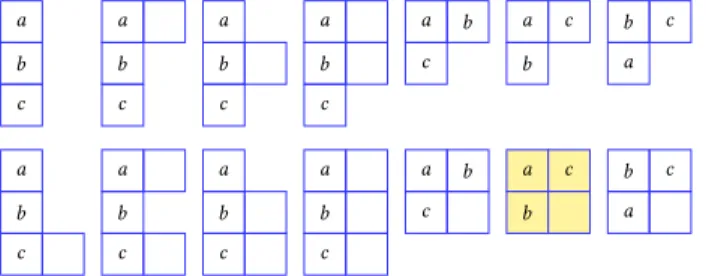
Example 3.2. Figure8shows all 14 possible states over the setA={a,b,c}of vertices withp=2.

In each case, each row denotes one partition set and hence the order of rows and the order of squares in a row does not matter. Empty squares correspond to the possibility of extension of the set, as defined

a b c a b c a b c a b c a b c a b c a b c a b c a b c a b c a c b a c b b c a b c a

Fig. 8. All possible states overA={a,b,c}withp=2

a c b d e f

→

Fig. 9. Two compatible states overA={a,b,c}andA′={d,e,f}

bysz. The optimal2-partitioningψ presented in Figure7realizes the highlighted state in Figure8,

becauseψputsaandcin the same partition and putsbin a partition of size2, whose other member,d,

comes from outside the set{a,b,c}.

Compatibility.We say that two statessands′, respectively over the setsAandA′, are compatible

if there exists ap-partitioning that realizes both of them. We writes ⇆s′to show compatibility.

Example 3.3. Intuitively, two states are compatible if they can fit into each other. Figure9shows

the states realized by the2-partitioning of Figure7above over the setsA={a,b,c}andA′={d,e,f}

and how they can be fitted together to create the entire2-partitioning.

Algorithm1.We are now ready to describe our algorithm in detail. Given a graphG, a weight

functionwand an optimal nice tree decompositionT ofG, our algorithm performs a bottom-up

dynamic programming onT. This is broken into three steps.

Step 0: Initialization.We define several variables at each node of our treeT. These variables are

meant to be computed in a bottom-up manner. Concretely, for everyt ∈T and every statesover

the bagX_t, we define a variabledp[t,s]and initialize it to+∞.

Invariant.Formally, our algorithm satisfies the following invariant for everydpvariable right after the end of its computation:

dp[t,s]= The minimum total weight of cross edges over allp-partitionings ofG_t that realizes.

Intuitively, we are considering the states over the bagX_t and extending them by adding vertices

that were introduced in the subtree oftinT.

Step 1: Computation ofdp.The algorithm starts from the bottom of the treeT and computes the

dpvariables bottom up, i.e. with an order such that for every nodet ∈T thedpvariables at its

children are computed before thedpvariables oft. For every nodet ∈T and states=(φ,sz) ∈S_X

t,

we show howdp[t,s]is computed based on the type of the nodet:

(1.1) iftis a Leaf:dp[t,s]=0;

(1.2) iftis a Join node with childrent1andt2: dp[t,s]= min

sz1+sz2≡sz

Note that the summation and equality above are pointwise.

(1.3) iftis an Introduce Vertex node, introducingv, with a single childt1:

dp[t,s]=dp[t1,(φ|X_t

1,sz|Xt1)]

;

(1.4) iftis an Introduce Edge node, introducinge, with a single childt1:

dp[t,s]=dp[t1,s]+w(e,φ),

wherew(e,φ)is equal tow(e)ifeis a cross edge inφand zero otherwise; (1.5) iftis a Forget Vertex node, forgettingv, with a single childt1:

dp[t,s]= min s′_∈S

Xt1

∧s′_⇆sdp[t1,s

′_].

Recall that⇆denotes compatibility.

Step 2: Computing the Output.The algorithm computes the output, i.e. the optimal weight of a

p-partitioning, using the values stored atdpvariables. Ifris the root node ofT, then the algorithm

outputs the following value: min_s∈S

Xr dp[r,s].

This concludes Algorithm1. We now prove the correctness of our algorithm.

Lemma 3.2. Algorithm1correctly computes the total weight of cross edges in a minimum-weight

p-partitioning.

Proof. We prove this lemma in two steps. First, we show that the invariant defined above

holds after computingdp[t,s]assuming that it was satisfied for alldpvariables in the children oft

(Correctness of Step 1). Then, assuming that the invariant holds fordpvariables at the root, we

show that the output is the total weight of an optimalp-partitioning (Correctness of Step 2).

Intuitively, the invariant says that if we only consider the graphG_t, i.e. the part ofGthat was

introduced in the subtree ofT rooted att, and thosep-partitionings ofG_t that realize the states,

thendp[t,s]holds the minimum total weight of cross edges among thesep-partitionings.

Correctness of Step 1.As in the algorithm, we break this part into several cases:

(1.1) Computations at Leaves.The nodetis a leaf inT, henceG_tis the empty graph andX_t is the

empty set. Therefore,S_X

t contains a single trivial states∅and we havedp[t,s∅]=0 because

the total weight of cross edges in an empty graph is zero.

(1.2) Computations at Join Nodes.The nodet is a join node with childrent1andt2. We want to

computedp[t,s]wheres =(φ,sz). Therefore, we only consider thosep-partitionings that

realizes. Given thatX_t =X_t

1 =Xt2,φimposes itself on bothXt1 andXt2. However, each

partition inφmust be extended by a number of vertices as defined bysz. These vertices

must come from eitherG_t

1orGt2and must not already be present inXt. According to the

separation lemma (Lemma2.1), the only vertices that are in bothG_t

1andGt2are precisely those

ofX_t. Hence, each new vertex comes either fromG_t

1orGt2but not from both. Therefore, we

should minimize our total cross edge weights wrtdpvariables of the formdp[t1,(φ,sz1)]and dp[t2,(φ,sz2)]wheresz1+sz2≡sz. The functionsz1defines the number of vertices that should

be added fromG_t

1−Xtto each partition ofφandsz2does the same forGt2−Xt. Formally, if

we letw(φ)be the total weight of cross edges caused byφinG_t

1∩Gt2 =Gt1[Xt] ∩Gt2[Xt],

then we should let:

dp[t,s]=dp[t,(φ,sz)]= min sz1+sz2≡sz

dp[t1,(φ,sz1)]+dp[t2,(φ,sz2)] −w(φ).

The reason we are subtractingw(φ)at the end is that the weights of its corresponding edges

We now show it is always the case thatw(φ)=0. If an edge contributes tow(φ), then it must

be present in bothG_t

1andGt2. However, by property (3) of a nice tree-decomposition, each

edge is introduced exactly once. Hence,G_t

1 andGt2 do not share any edges andw(φ)=0.

Therefore, by settingdp[t,s]=dp[t,(φ,sz)]=min_sz

1+sz2≡szdp[t1,(φ,sz1)]+dp[t2,(φ,sz2)],

we satisfy the invariant.

t

t1 t2

Fig. 10. In a join nodet,Gt1andGt2do not share any edges and their shared vertices are inXt.

(1.3) Computations at Introduce Vertex Nodes.The nodetis an introduce vertex node. So, it has

a single childt1andXt =Xt1∪ {v}for somev <Xt1. We know that the vertexv cannot

possibly appear inG_t

1because every vertex appears in a connected subtree ofT andv<Xt1.

Hence,G_t is obtained by addingvas an isolated vertex toG_t

1. Again, we want to compute

dp[t,s]and should hence only consider thep-partitionings that realizes. Given thatX_t

1 ⊂Xt,

simposes a unique compatible state onX_t

1. Moreover,Gthas no new edges in comparison

withG_t

1, so the total weight of cross edges should only be computed inGt1. Hence, we let

dp[t,s]=dp[t,(φ,sz)]=dp[t1,(φ|X_t

1,sz|Xt1)].

Intuitively, this is equivalent to removingvfrom its partition and then computing thedpint1.

t t1

Fig. 11. In an introduce vertex nodet, the newly introduced vertex is isolated and there are no new edges.

(1.4) Computations at Introduce Edge Nodes.The nodethas a single childt1andXt =Xt1. Moreover,

the only difference betweenG_t andG_t

1 is in a single edgee. When computingdp[t,s], the

statesforces itself onX_t

1 =Xt. Hence we should letdp[t,s]=dp[t1,s]+w(e,s), wherew(e,s)

is the contribution of the edgeeto the total weight of cross edges ins. It is zero if the two

sides ofeare put in the same partition set bysand is equal tow(e)otherwise.

t t1

Fig. 12. A new edge is introduced in the nodet. The states are only dependent on vertices and hence are the

same overXt andXt1. However, we have to account for the weight of the new edge.

(1.5) Computations at Forget Vertex Nodes.In this case the nodethas a single childt1andXt =

to take the minimum among the values ofdp variables of all statess′overX_t

1 that are

compatible withs. More precisely, we letdp[t,s]=min_s′_∈S Xt1

∧s′_⇆sdp[t1,s ′_].

t t1

Fig. 13. When a vertexvis forgotten byt, we haveGt=Gt1, butXt =Xt1\ {v}.

Correctness of Step 2.Given thatr is the root node ofT, we haveG_r = G. Since everyp

-partitioning ofGrealizes some state overX_r, it follows that the optimal weight of ap-partitioning

is min_s∈S

Xr dp[r,s]. This concludes the proof.

□

Remark 3.1. Algorithm 1 computes the total weight of cross edges in a minimum-weightp

-partitioning. As is common with dynamic programming algorithms, an optimalp-partitioning itself can be obtained by keeping track of the choices made during the computation ofdpvariables, i.e. keeping track of the cases that led to the minimal values in each computation.

We now establish the complexity of our approach and present the main theorem of this section. Number of States.For a fixedp, letCp

k denote the number of different possible states over a set of

sizek, i.e.Cp

k :=|S_{1,2, ...,k}|. We writeCkinstead ofC p

k whenpcan be inferred from the context.

AppendixAestablishes bounds on the value ofC_k. Note that this value only depends onpandk.

Theorem 3.1. Given a Data Packing instanceI =(n,1,p,R)as input, wherenis the number of

distinct data elements,pis the packing factor,Ris the reference sequence with a length ofN and the cache has unit size, the Data Packing problem, i.e. finding the minimal number of cache misses, can be solved in linear time, i.e. in timeO(N+n·k2

·C_k ·pk), when the underlying access graphGR has treewidthk−1.

Proof. Given a Data Packing instanceI =(n,1,p,R), we first apply the reduction of Lemma3.1

which takesO(N). We then use Algorithm1to solve the resulting minimum-weightp-partitioning

problem. The correctness of this algorithm was established in Lemma3.2. The only remaining

part is to find the runtime of Algorithm1. Note that the time spent for computing a nice tree

decomposition, as in Lemmas2.2and2.3are linear and dominated by the rest of our runtime.

The algorithm needs values ofdpvariables for all nodes of the tree decomposition which are at

mostO(n·k). We obtain upper-bounds for the runtime of our algorithm on each type of node:

• Leaves.There is a single state at each leaf and itsdpis zero. Hence we spendO(1)at each leaf.

• Join Nodes.At a join nodet, there are at mostC_kstates and for each states =(φ,sz)we have

to look into the states corresponding to every possible size enlargement functionsz1≤sz. As

in the proof of LemmaA.2, there are at mostpksuch functions. Creating each corresponding

state takesO(k). Hence, we spendO(k·C_k·pk)at each join node.

• Introduce Vertex Nodes.At a nodet, there areC_kstates and we spendO(k)computing the

unique corresponding state overX_t

1. Thus, each introduce vertex node takesO(k·Ck). • Introduce Edge Nodes.This case is similar to the previous one and takesO(k·C_k).

• Forget Vertex Nodes.At a nodet, there areC_kstates and for each of them we have to look into all its compatible states overX_t

1. Note that such compatible states can be obtained either by

by adding it to the partition set of another vertex inX_t. Hence, there are at mostp+ksuch states and the total processing time of a forget vertex node isO(k· (p+k) ·C_k).

Note that the runtime for join nodes dominates the rest. Given that there areO(n·k)nodes in

total, the whole computation takesO(n·k2·C_k·pk)time. Finally, the algorithm spendsO(C_k)time

computing the final result using thedpvalues at the root. □

Remark 3.2. By exploiting treewidth, we provided alinear-timealgorithm for finding the exact

solution to the Data Packing problem whenm=1. Note that in the general case, i.e. without considering

parameterization by treewidth, this problem is NP-hard as mentioned in Theorem2.1.

Remark 3.3. We assumed LRU as the replacement policy. However, given that the replacement

policy does not matter when the cache has unit size (Remark2.1), our algorithm is applicable to any replacement policy, including FIFO and OOP.

3.2 Hardness of Data Packing on Trees

In this section, we provide a reduction from the general problem of Data Packing to the special case where the access graph is a tree, i.e. has treewidth 1. This reduction leads to hardness results

that enhance those of [Lavaee 2016] by showing that the problem remains hard even on trees. This

indicates that although considering constant treewidth access graphs led to efficient algorithms for

the case ofm=1, constant treewidth access graphs alone are not sufficient form≥2.

Theorem 3.2 (Hardness of Data Packing on Trees). Given a Data Packing instanceI =

(n,m,p,R), we have the following hardness results:

• Hardness of the Exact Problem.For anym≥2and anyp≥3, Data Packing is NP-hard even if

the underlying access graphGRis a tree.

• Hardness of Approximation.Unless P=NP, for anym≥6,p ≥2and any constantϵ >0, there

is no polynomial approximation algorithm for the Data Packing problem with an approximation factor ofO(N1−ϵ)even if the access graphGRis a tree.

Proof. We provide a linear-time reduction that transforms a Data Packing instance I =

(n,m,p,R)to another instanceI′ = (n+(m+1)p,m+1,p,R′)such that the access graphG_R′

is a tree. Both hardness results can then be obtained by applying this reduction to the hardness results of Section2.1. GivenI, we introduce(m+1)pnew data elementsd1,d2, . . . ,d(m+1)p. LetX be the sequenced1,d2, . . . ,d(m+1)p,d(m+1)p−1, . . . ,d1.We form the sequenceR

′_{as follows:}

d1,R[1],d1,R[2],d1, . . . ,d1,R[N],d1,X,X, . . . ,X

| {z }

2N+m+2 times

,

i.e. we takeR and addd1 at its beginning, end and between every two elements of it, then we

concatenate the result with 2N +m+2 copies ofX. We letI′=(n+(m+1)p,m+1,p,R′). Note

that the cache inI′has one spot more than the cache ofI.

By construction,G_R′is a tree, because it consists of a pathd1, . . . ,d(m+1)pand every other vertex

of the graph is only connected tod1. We now show that the optimal number of cache misses inI

′ is

exactlym+1 plus the optimal number of cache misses inI.

Letσbe an optimal data placement scheme forI′, thenσmust necessarily put thed_i’s in exactly

m+1 blocks, otherwise eachX in the sequenceR′will lead to at least one cache miss for a total of

at least 2N+m+2. On the other hand, putting thed_i’s inm+1 blocks leads to at most 2N+m+1

cache misses, even if all accesses before theX’s are missed. In particular,σdoes not put any element

ofRin the same block asd1. Therefore,σ first leads to a cache miss on the first access tod1, then

keepsd1in the cache forever. Hence,σfills one spot of the cache with the block ofd1and hasm

Hence, the number of cache misses caused byσis 1 (for the firstd1) plus the optimal number of

misses inI plusm(for theX’s). □

Remark 3.4. As mentioned before, we are considering the LRU replacement policy in this paper.

However, the reduction above works for the OOP replacement policy as well. Hence, the hardness results are established for both policies.

4 DATA PACKING ON CONSTANT-TREEWIDTH ACCESS HYPERGRAPHS

In this section, we exploit constant treewidth of higher-order access hypergraphs for solving Data

Packing. Section4.1extends our linear-time algorithm to everym, when the access hypergraph of

orderq∗:=(m−1)p+2 has constant treewidth. As indicated by Theorem2.1, this problem is hard

to even approximate in the general case. In Section4.2we argue thatq∗is the optimal order for

exploiting treewidth in the sense that the problem remains NP-hard even if the access hypergraph

of orderq∗−1 has constant treewidth. This also leads to a new hardness-of-approximation result.

4.1 Algorithm for Constant-treewidth Access Hypergraph

In this section we extend the algorithm of Section3.1to any cache sizem, provided that the

hypergraphGq

∗

R is of constant treewidth, whereq∗=(m−1)p+2. Note that Theorem3.2implies

such an extension cannot be made if we only consider constant-treewidthG_R.

Intuition on Cache Misses.The main intuition behind our algorithm is the following: given an

instanceI =(n,m,p,R)and a data placement schemeσ forI, we can deduce whether an access

R[i]leads to a cache miss by looking at only the(m−1)p+1=q∗−1 previous accesses todistinct data elements. We now formalize this intuition.

Previous Access of a Block.Consider a Data Packing instanceI =(n,m,p,R), a data placement schemeσ forI and an accessR[i]. LetB :=[R[i]]_σ be the block ofσcontainingR[i]. We define

prev_σ(i)as the index of the previous access toB or 0 if no such access exists, i.e.prev_σ(i) :=

max{j<i |j=0∨ [R[j]]_σ =[R[i]]_σ}.

Lemma 4.1. Given a data placement schemeσ forI, an accessR[i]leads to a cache miss if and

only ifprev_σ(i)=0or there are at leastmdistinct blocks ofσwhose elements appear in the range

R[prev_σ(i)+1]. . .R[i−1].

Proof. We are assuming LRU as the replacement policy and the cache starts empty. Ifprev_σ(i)=

0, thenR[i]is the first access to its block and will definitely lead to a cache miss. We now consider

the case whereprev_σ(i)_,0. Letj:=prev_σ(i)and assume thatB:=[R[i]]_σ =[R[j]]_σ is the block containingR[i]andR[j]. By definition, none of the elementsR[j+1], . . . ,R[i−1]belong toB. If

there are at mostm−1 blocks betweenR[j+1]andR[i−1], thenR[i]cannot lead to a cache

miss. This is because right after the accessR[j], the blockBis present in the cache and is the most

recently used block of the cache. Hence, in order for it to be evicted, at leastmother blocks must

be accessed. On the other hand, if there are at leastmblocks betweenR[j+1]andR[i−1], then

all of these blocks will be loaded into the cache and henceBwill be evicted before the accessR[i]

leading to an eventual cache miss onR[i]. □

Corollary 4.1. Given a data placement schemeσ, an accessR[i]and theq∗−1distinct elements

that were accessed beforeR[i](or all of the previous distinct elements if there is less thanq∗−1of

them) in the order of their last access time, one can deduce whetherR[i]leads to a cache miss.

Proof. IfR[prev_σ(i)]is one of these previous elements, then we can simply check whether at

leastmdifferent blocks appear betweenR[prev_σ(i)]andR[i]. Otherwise, eitherR[i]is the first access to its block or all theq∗−1 elements are appearing betweenR[prev_σ(i)]andR[i]. In the

first caseR[i]leads to a cache miss. In the second case, by pigeonhole principle, there are at leastm blocks between the two elementsR[prev_σ(i)]andR[i]and hence there is a cache miss atR[i]. □

Remark 4.1. Note that the previous access to the block containingR[i]might be an access toR[i]

itself. Hence,R[i]might itself appear in theq∗−1distinct elements that were accessed beforeR[i].

As in Section3.1, we are going to reduce Data Packing to a graph problem and then exploit

treewidth to obtain a linear-time algorithm. Corollary4.1suggests that in order to detect cache

misses, one only needs to consider the ordered access hypergraph of orderq∗ =(m−1)p+2,

i.e.Gˆq

∗

R . However, in order to address the corner case mentioned in Remark4.1, we define an ordered

hypergraphGby a slight change to the edges ofGˆq

∗

R and then reduce Data Packing to a graph

problem overG.

The Ordered HypergraphG.We define the ordered hypergraphGas having the same vertices

and edges as the ordered access hypergraphGˆq

∗

R, except in the following case:

• Given an accessR[i]to a data elementd, letR[j]be the last access beforeR[i]to the same data elementd. If there are at mostq∗distinct data elements accessed in the rangeR[j+1]. . .R[i−1], then the edgee_i corresponding toR[i], will also containR[j](in its natural position according to the order of vertices ine_i).

Example 4.1. Consider the access sequenceR=<d,c,a,b,c >and letm=p=2. Hence, we have

q∗_{=(m−1)p+2=4. In the graph}Gˆq

∗

R the edge corresponding to the secondcise5=<d,a,b,c >.

However, there are less thanq∗_{distinct data elements appearing between the two accesses toc, i.e. there}

are only two such elements, namely,aandb. Hence, inG, the previous access tocappears in this edge as well. Therefore, inG, the edgee5is of the forme5=<d,c,a,b,c>.

The intuition behind the wayGis defined comes from Corollary4.1and Remark4.1. The idea is

to have the edgee_i contain all the data necessary to decide whether a cache-miss will happen at

the accessR[i]. We now formalize this concept.

Missed Edges.Given an ordered hyperedgee_i ofGand a data placement schemeσ, we can deduce

whether a cache miss happens atR[i]using Corollary4.1, because the edgee_i contains an ordered

list of at least(m−1)p+1=q∗−1 distinct data elements that were accessed right beforeR[i]. We

say that an ordered hyperedgee_i is missed inσ, if the correspondingR[i]is a cache miss.

Identifying Missed Edges.Consider the data placement schemeσas ap-partitioning of vertices ofG. Based on Lemma4.1and Corollary4.1, an ordered hyperedgee_i =<v1, . . . ,vl >is missed iff the sequence of vertices<v_l,v_l−1, . . . ,v1 >inGvisits at leastmdistinct partitions before getting

back to the partition[v_l]_σ or if it never comes back. Note that this determination can be done in

O(m·p)and only depends on thep-partitioning of{v1, . . . ,vl}. We now define our graph problem as follows:

Minimum-missp-partitioning.Given a hypergraphG=(V,E)with ordered hyperedges,

parti-tionV into sets of size at mostpin a manner that minimizes the number of missed edges.

As a direct result of the previous discussion, we have the following lemma:

Lemma 4.2. The optimal number of cache misses in a Data Packing instanceI =(n,m,p,R)is equal

to the optimal number of missed edges in ap-partitioning ofG.

Proof. Any data placement schemeσ forI is also ap-partitioning ofG. As shown above,σ

misses an edgee_i inGiff it causes a cache miss atR[i]inI. Hence, the number of cache misses

States over a Set of Vertices.We define states in the exact same manner as in Section3.1, i.e. a

state over a setAof vertices is a pairs =(φ,sz)consisting of an equivalence relationφand a size

enlargement functionsz. The concepts of realization and compatibility are also defined similarly.

Algorithm2.We now provide a linear-time algorithm for solving the Minimum-Missp-partitioning

problem, assuming that the hypergraphGhas constant treewidth. The algorithm is an extension

of the one provided in Section3.1. In the following, we let(T,{X_t|t∈T})be an optimal nice tree

decomposition ofG. Our algorithm performs a bottom-up dynamic programming onT.

Step 0: Initialization.We define several variables at each node of the treeT. Concretely, for every nodet∈T and every statesoverX_t, we define a variabledp[s,t], initially holding a value of+∞. Invariant.The most different aspect of our algorithm compared to Section3.1is the invariant.

Formally, we require our algorithm to satisfy the following invariant for everydpvariable right

after the end of its computation:

dp[t,s]:= The minimum number of missed edges over allp-partitionings ofG_tthat realizes.

Step 1: Computation ofdp.Thedpvariables are computed in a bottom-up manner. Given a node

t ∈T and a states =(φ,sz) ∈S_X

t, we show howdp[s,t]is computed in terms of thedpvariables

at the children oft. This computation depends on the type of the nodet.

(1.1) iftis a Leaf:dp[t,s]=0;

(1.2) iftis a Join node with childrent1andt2: dp[t,s]= min

sz1+sz2≡sz

dp[t1,(φ,sz1)]+dp[t2,(φ,sz2)]; (1.3) iftis an Introduce Vertex node, introducingv, with a single childt1:

dp[t,s]=dp[t1,(φ|X_t

1,sz|Xt1)]

;

(1.4) iftis an Introduce Edge node, introducinge, with a single childt1: dp[t,s]=dp[t1,s]+

1 missed_edge(e,φ)

0 otherwise

;

(1.5) iftis a Forget Vertex node, forgettingv, with a single childt1: dp[t,s]= min

s1∈S_Xt 1∧s1⇆s

dp[t1,s1].

Recall that⇆denotes compatibility of states.

Step 2: Computing the Output.The algorithm computes the output, i.e. the minimum number

of missed edges in ap-partitioning ofG, using the values ofdpvariables at the root noder ofT.

Formally, the output is min_s∈S

Xrdp[r,s].

This concludes Algorithm2. While most of the computations are similar to Algorithm1, the

argument for correctness of Algorithm2and its runtime are rather different. We first prove the

correctness of our approach and then establish its time complexity.

Lemma 4.3. Algorithm2correctly computes the total number of missed edges in a Minimum-Miss

p-partitioning.

Proof. Our proof heavily depends on the invariant defined above. Intuitively, the invariant says

thatdp[t,s]must be filled with the minimum number of edges that are missed in ap-partitiong

realizings, over the subgraphG_t ofG, which consists of all the vertices and hyperedges that are

introduced belowtinT. We prove the lemma in two steps. First, we prove that the invariant is