Using convolutional neural networks for classification of malware represented as images

http://hdl.handle.net/10459.1/67672

The final publication is available at:

Copyright

(will be inserted by the editor)

Using Convolutional Neural Networks for Classification of

Malware represented as Images

Daniel Gibert · Carles Mateu · Jordi Planes · Ramon Vicens

Received: date / Accepted: date

Abstract Malware authors introduced obfuscation tech-niques to existing malware in order to evade detection and hide its purposes. As a result, the number of ma-licious programs has grown in both volume and so-phistication. Thus, effective categorization of malware based on its characteristics and behavior is required. In this paper, malicious software is visualized as gray scale images since its ability to capture minor changes while retaining the global structure helps to detect vari-ations. Motivated by the visual similarity between mal-ware samples of the same family, we propose a file ag-nostic deep learning approach for malware categoriza-tion to efficiently group malicious software into fami-lies based on a set of discriminant patterns extracted from their visualization as images. The suitability of our approach is evaluated against two benchmarks: the MalImg dataset and the BigData Innovators Gather-ing. Experimental comparison demonstrates its supe-rior performance with respect to state-of-the-art tech-niques.

Keywords Malware Visualization, Malware Classifi-cation, Convolutional Neural Network, Deep Learning

Corresponding author: D. Gibert Blueliv, Leap in Value, Barcelona, Spain Tel.: +34 654 252 008

E-mail: [email protected] C. Mateu

University of Lleida, Lleida, Spain E-mail: [email protected] J. Planes

University of Lleida, Lleida, Spain E-mail: [email protected] R. Vicens

Blueliv, Leap in Value, Barcelona, Spain E-mail: [email protected]

1 Introduction

Malware, short for malicious software, refers to software programs designed to perform any kind of unwanted or harmful action on a computer system. Malware can be divided into the following categories, not mutually exclusive, depending on their purpose:

– Adware. It is designed to automatically render ad-vertisements. Advertising-supported software often comes bundled with software and applications and serves as a revenue tool.

– Spyware. It spies and gathers user information with-out their knowledge and permission. Spyware pro-grams are used to record keystrokes, to harvest fi-nancial data or monitoring user activity.

– Virus. It is capable of reproducing itself and spread-ing to other computer systems.

– Worm. It exploits vulnerabilities of the operation system to spread. The major difference between worms and viruses is the ability of worms to independently self-replicate and spread while viruses depend on hu-man activity.

– Trojan. It disguises itself as a benign program to deceive users.

– Rootkit. It is designed to enable remotely access to a computer or its software without permission.

– Backdoor. It is designed to bypass system’s security mechanisms.

– Ransomware. It essentially restricts user access to the computer by encrypting the files or locking down the system while demanding a ransom.

– Bot. They are created to automatically perform spe-cific operations such as DDoS attacks or malware distribution.

Moreover, malicious software can be grouped to-gether into families depending on their behavior and capabilities and, consequently, these shared character-istics between samples belonging to the same family might be used for detection and classification of unseen programs.

According to McAfee [15] more than 600 million types of malware were detected during the first quarter of 2017. The proliferation of malicious software has in-creased quickly thanks to the utilization of polymorphic and metamorphic techniques used to evade detection and hide its malicious purpose. On the one hand, poly-morphic malware uses a polypoly-morphic engine to mutate the code while keeping the original functionality intact. Packing and encryption are the two most common ways to hide code. On the other hand, metamorphic mal-ware rewrites its code every time it is propagated to an equivalent one. Traditionally, antivirus solutions relied on signature-based and heuristic-based methods. A sig-nature is an algorithm or hash that uniquely identifies a specific malware. Heuristics is a set of rules determined by experts after analyzing the behavior of malware. The main drawback of both approaches is that the malware has to be analyzed prior to the creation of these rules and heuristics. Broadly speaking, there are two kind of approaches: static analysis and dynamic analysis.

Static analysis consists of examining the code or structure of a program without executing it. This kind of analysis can confirm whether a file is malicious, pro-vide information about its functionality and can also be used to produce a simple set of signatures. The most common static analysis approaches are:

– Finding sequences of characters or strings. Search-ing through the strSearch-ings of a program is the most sim-ple way to obtain hints about its functionality. For instance, you can find strings related to printed mes-sages, URLs to which the program accesses, the lo-cation of files modified by the executable and names of common Windows dynamic link libraries (DLLs).

– Analysis of the Portable Executable File Format. The Portable Executable(PE) file format is used by Windows executables, object code and DLLs. Among the information it includes, the most use-ful pieces of information are the linked libraries and functions as well as the metadata about the file in-cluded in the headers.

– Searching for packed/encrypted code. Malware writ-ers usually use packing and encryption to make their files more difficult to analyze. Software programs that have been packed or encrypted usually contain very few strings and higher entropy compared to legitimate programs.

– Disassembling the program, i.e. recovering the sym-bolic representation from the machine code instruc-tions.

Dynamic analysis involves executing the program and monitoring its behavior on the system. Unlike static analysis, dynamic analysis allows to observe the actual actions executed by the a program. It is typically per-formed when static analysis has reached a dead end, either due to obfuscation and packing, or by having exhausted the available static analysis techniques. A survey on automated dynamic analysis techniques and tools is found in M. Egele et al [6]. Some techniques are:

– Function Call Monitoring. The behavior of the pro-gram is analyzed by using the traces containing the sequence of functions invoked by the executable un-der analysis.

– Function Parameter Analysis. Consists of tracking the values of parameters and function return values.

– Information Flow Tracking. Analyze how a program processes data and how data is propagated through the system.

– Instruction Trace. Analysis of the complete sequence of machine instructions executed by the program. However, both static and dynamic analysis tech-niques have their own drawbacks. Static analysis is faster but suffers from code obfuscation, techniques used by malware authors to conceal the malicious purpose of the program. Dynamic analysis does not need to unpack or decrypt the executable but is more resource-consuming. Additionally, both approaches require past detection of the malware to generate signatures. Unfortunately, such systems fail to predict new unseen malware and it is unfeasible to analyze manually every sample received. Thus, techniques to automatically categorize malware are required.

Recently, machine learning techniques have been em-ployed as a solution against malware. The success of these approaches has increased thanks to: (1) the rise of commercial feeds of malware; (2) the reduction in cost of computing power; and (3) the advances made in the machine learning field. Several methods have been ap-plied based on features extracted from both static and dynamic analysis. A review of the most common fea-tures used by machine learning techniques is presented in Section 2.

Based on the work of Nataraj et al. [19], in this paper we present a file agnostic deep learning system to classify malware into families based on the repre-sentation of their binary content as gray-scale images. Our work is based on the observation that samples of the same family appear to be visually similar while dis-tinct from samples of other families. To demonstrate

the suitability of our novel approach we make use of two publicly available datasets, one containing 9458 samples of 25 different malware families and a second contain-ing 10868 samples of 9 different families. Experiments show that our method is capable of classifying samples from both datasets with 98.48% and 97.49% of accu-racy, respectively, outperforming state-of-the-art meth-ods in the literature.

The rest of the paper is organized as follows: Section 2 discusses the related research. Section 3 describes the insights from representing malicious software as gray scale images. Section 4 introduces our deep learning approach for malware classification. Section 5 evaluates the performance of our method. Finally, Section 6 con-cludes with our remarks and future work suggestions.

2 Related Work

The use of machine learning algorithms to address the problem of malicious software detection and classifica-tion has increased during the last decade. An overview is provided in [22, 7]. Instead of directly digesting raw malware, machine learning solutions first extract fea-tures that provide an abstract view of the software pro-gram. Then the features extracted are used to train the model. The type of features can be broadly divided into two groups just like the types of malware analysis.

Static features are those extracted from the binary of the malware without executing it. One of the most common types of features is byte n-grams. An n-gram is a contiguous sequence of n items from a given sequence of text. In the work of Tesauro et al. [28] they extracted a list of byte-sequence trigrams and used an artificial neural network to classify malware. Similar to byte-sequence n-grams, approaches in the literature have used opcodes n-grams [24, 4]. An opcode (abbreviated from operation code) is the portion of machine language instruction that specifies the operation to be performed. In particular, D. Yuxin et al. [29] used deep belief net-works as a feature extractor to generate deep features to represent executables from their opcodes sequences. Features can also be extracted from the Portable Exe-cutable (PE) Header. The PE Header contains informa-tion about the files themselves such as the associated dynamically linked libraries and the sections of the pro-gram and their sizes. For instance, Ravi and Manoharan et al. [5] proposed a malware detection system based on Windows API call sequences. In addition, entropy has proven to be an effective feature to detect malware. The entropy of a program, refers to the amount of disorder (uncertainty) or its statistical variation. Entropy has commonly been used to detect encrypted and packed executables because these programs often have higher

entropy. For example, in the dataset studied by Lydia et al. [16], native executables had an average entropy of 5.099 while packed and encrypted executables had an average entropy of 6.801, 7.175, respectively. Moreover, Bat-Erdene et al. [3] used entropy analysis to classify packing algorithms of given unknown packed executa-bles.

Furthermore, dynamic features are those extracted by executing and observing the behavior of malware. Malware API calls have been used to model the be-havior of malware. In [23], Z. Salehi et al. constructed dynamic features based on the name of API calls and each argument and return value recorded in a controlled environment during runtime. M. Ghiasi et al. [8] pre-sented a framework for malware detection based on the changes in register contents. In [27], C.Storlie et al. presented a spine logistic regression model for mal-ware detection, trained on the instruction traces ex-tracted dynamically from computer programs. Addi-tionally, B.Anderson [2] constructed graphs from the instruction traces of executables and applied graph ker-nels to create and compare similarity matrices of differ-ent computer programs.

Besides, several visualization techniques have been proposed in the literature to help malware analysis. Nataraj et al. [19] used image processing techniques to classify malware according to its visualization as grayscale images. Their method represented a binary file as a grayscale image by converting each bit value into an image pixel. Han et al. [9] converted the images into entropy graphs. Their system used the bitmap im-age to calculate the entropy value of each line and gen-erate an entropy graph. Lastly, Sorokin et al. [25] visual-ized a given executable using its structural entropy, ob-tained by dividing a binary into non-overlapping chunks and computing the entropy for each chunk.

3 Malware Visualization

Our approach is motivated by the results of the exper-iments of Nataraj et al.[19]. Their work is based on the observation that images of malware samples from the same family appear to be similar while distinct from samples belonging to different families.

3.1 Visualizing Malware as an Image

To visualize a malware sample as an image, every byte has to be interpreted as one pixel in an image. Then, the resulting array has to be organized as a 2-D array and visualized as a gray scale image. In our work, we tried to keep an aspect ratio of 3:2. Note that the resulting

gray-scale images will have distinct widths and heights because the size of each sample is different. Values are in the range [0,255] (0:black, 255:white).

Fig. 1 shows the representation of samples of mal-ware belonging to nine different families as gray-scale images. It can be observed that images of software ex-ecutables from a given family are similar visually while distinct from those belonging to a different family. The main benefit of visualizing a malicious executable as an image is that the different sections of a binary can be easily differentiated. In addition, malware authors only used to change a small part of the code to produce new variants. Thus, if old malware is re-used to create new binaries the resulting ones would be very similar. Additionally, by representing malware as an image it is possible to detect the small changes while retaining the global structure of samples belonging to the same family.

Fig. 1: Gray-scale images of malicious software belong-ing to various families. Note that the images of malware belonging to the same family are similar while distinct from the images of malware from the rest of families.

In most cases, when observed in detail, one can notice several sections in the program, which usually have distinct feature patterns. Furthermore, the im-ages stored in the resources section (.rsrc) of the PE file are also displayed (See Fig. 2). In addition, with this kind of representation you can detect where zero-padding has been applied. Zero-zero-padding is mainly used for block alignment but malware authors also use it to reduce the overall entropy of an executable.

Fig. 2: Gray-scale image representation of a malware sample containing a logo on their resources section

3.2 Texture Analysis and Feature Extraction

Traditional recognition approaches are composed of two stages: (1) feature extraction, transforming an observed signal into a robust representation, and (2) classifica-tion to model decision-making. Consequently, their per-formance relies heavily on the discriminative power of the features extracted. Image-based hand-designed fea-ture extractors in the literafea-ture [19, 1, 18] gather rele-vant information about an input and eliminate irrele-vant variabilities. In summary, Nataraj et al. [19] and Narayanan et al. [18] extracted GIST and PCA fea-tures, respectively, and Ahmadi et al. [1] extracted both Haralick and local binary pattern features. Below is a brief description of the aforesaid methods.

GISTdescriptors [21]. Given an image, the process to compute a GIST descriptor is as follows. First, the image is convolved with 32 Gabor filters with 8 orienta-tions and 4 scales. Second, each feature map is divided into 16 regions of 4x4 values, and then the feature values are averaged within each region. Last, the 16 averaged values of all feature maps are concatenated.

PCA [11] features. Principal Component Analysis is a statistical procedure used for dimensionality reduc-tion. It uses an orthogonal transformation to convert a set of observations ofn possible correlated variables into a set of values with m linearly uncorrelated vari-ables named principal components, wheren≤m.

Haralick[10] features. Haralick features have been used for image classification for years. The features are

calculated by constructing a co-occurrence matrix. Then, they are computed by using the equations defined by Haralick such as the angular second-moment, contrast, correlation, etc.

Local binary pattern[20] features. The local bi-nary pattern (LBP) feature of a given pixel is computed as follows. First, an 8 bit binary array is initialized as 0. Then, each pixel is compared with its neighboring pixels in clockwise direction. If the value of the neigh-boring pixel is greater or equal 1 is assigned to its corre-sponding position. This gives an 8 bit binary array with zeros and ones. The 8-bit binary pattern is converted to a decimal number and is stored in the corresponding pixel location in the LBP mask. This process is applied to all pixels in an image. Once all LBP values have been calculated, the mask is normalized, resulting in 256 features.

Following recent advances in the machine learning community, we propose a system that automatically ex-tracts local and invariant features with convolutional neural networks. Experiments in Section 5 demonstrate its superior performance in comparison to the afore-mentioned methods.

4 Convolutional Neural Networks for Malware Classification

Convolutional neural networks (CNNs) [14] are a type of artificial neural network biologically inspired by the mammals visual cortex [12], whose receptive field com-prises sub-regions layered over each other to cover the entire visual field. This type of networks has long been used in visual recognition tasks such as image classi-fication or object detection due to its ability to auto-matically extract discriminant and local features from images.

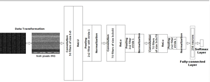
The core of a convolutional neural network consists of one or more convolutional layers and one or more fully connected layers. In particular, convolutional lay-ers act as detection filtlay-ers for the presence of specific features or patterns present in the data. The first layers detect lower level features whereas later layers detect increasingly high level features. On the contrary, fully connected layers are used at the end of a CNN to com-bine all the specific features detected by the previous layers and determine a specific target output. Figure 3 presents an overview of our CNN architecture.

The input of the network is an executable repre-sented as a grayscale imagexw,h,d, wherewandhare the width and the height of the image, respectively, and d is the depth (d = 1). Following the input layer are three 4-stage feature extractors which learn

hierar-chical features through convolution, activation, pooling and normalization layers.

1. Convolution. Convolution is a mathematical op-eration that takes an input signal of size w×h×d and a filter of size k×k×d, where k≤ w, h, and produces one output signal. The kernel slides over each value of the input signal, multiplies the corre-sponding entries of the input signal and the kernel and adds them up. Figure 4 presents three of the filters learned in the first convolutional layer. It can be observed that the features these kernels detect are high changes in the pixels intensities. In partic-ular, the convolutional layers are composed of 50, 70 and 70 filters of size 5x5x1, 3x3x50 and 3x3x70 for the first, second and third convolutional layers, respectively.

2. Activation function. The activation function is used to signal distinct identification of likely fea-tures. Specifically, we used the ReLU [17] non-linear functiony(x) =max(x,0) in all activation layers. 3. Pooling. The pooling operation reduces the spatial

size of the features and provides some sort of ro-bustness against noise and distortion. We applied max-pooling with filters of size 2x2x1 with stride 1, which reduces the input signal by half, i.e. if the input signal’s size is 128x128x1, the output of apply-ing max-poolapply-ing is an output signal of size 64x64x1. 4. Normalization. The input values for different neu-rons in the layer are normalized using local response normalization [13] to inhibit and boost the neurons with relatively larger activations.

At the end of the extractor, the feature maps are flat-tened and combined to be used as input of the follow-ing feed-forward layer composed of 256 neurons. Lastly, the output of the aforementioned layer passes to a soft-max layer to classify the binary program into its corre-sponding family. In addition to normalization, to pre-vent overfitting we employed dropout [26], a regular-ization mechanism which randomly drops a proportion of p units during forward propagation and prevents the co-adaptation between neurons.

5 Evaluation

This section presents an empirical evaluation of the re-sults obtained by our method in two datasets: (1) the MalImg dataset [19]; (2) the dataset provided by Mi-crosoft for the Big Data Innovators Gathering Anti-Malware Prediction Challenge.

Fig. 3: Convolutional neural network for classification of malware represented as gray-scale images. It is composed by 3 convolutional layers followed by one fully-connected layer. The input of the network is a malicious program represented as a gray-scale image. The output of the network is the predicted class of the malware sample.

Fig. 4: Images of 3 filters randomly selected from the first convolutional layer

5.1 Experimental Setup

The experiments were run on a single computer with the following hardware specifications:

– CPU: Intel i7-7700K

– Memory: 32 GB RAM

– GPU: Nvidia GTX 1080 Ti

To estimate the generalization performance of our ap-proach we used K-fold cross validation. The dataset is divided into K equal size folds. Of the K subsamples, a single subsample is retained as the validation data for testing the model and the remaining subsamples are used as training data. This procedure is repeated as many times as there are folds, with each of the K folds used exactly once as the validation data.

Furthermore, to select the best model, additional evaluation metrics have been used: precision, recall and F1 score. This is because accuracy can be a mislead-ing measure. Sometimes it may be desirable to select a model with a lower accuracy but with a greater pre-dictive power on the problem (aka. accuracy paradox). This occurs when there is as large class imbalance, where

a model can predict the value of the value of the major-ity class for all predictions and achieve a high classifi-cation accuracy while making mistakes on the minority or critical classes.

Precision (P) is defined as the number of true pos-itives (Tp) over the number of true positives plus the

number of false positives (Fp).

P = Tp Tp+Fp

Recall (R) is defined as the number of true positives (Tp) over the number of true positives plus the number

of false negatives (Fn).

P = Tp Tp+Fn

The F1 score is the weighted average of precision, de-fined as following:

F1= 2· P·R P+R

Since our target task is a multi-class classification prob-lem, we used an adapted version of the score named macro-averaged F1 score, defined as the average of the individual F1 scores obtained for each class.

macro F1= 1 q q X i=1 F1i

whereqis the number of classes in the dataset andF₁i is the F1 score of class i. Macroaveraging gives equal weight to each class. Thus, large classes will not domi-nate over small classes.

5.2 MalImg dataset

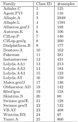
The MalImg dataset was provided by Nataraj et al. [19] and consists of 9342 gray scale images of 25 mal-ware families. It contains samples of malicious soft-ware packed with UPX from different families such as Yuner.A, VB.AT, Malex.gen!J, Autorun.K and Rbot!gen. Additionally, there are images of family variants like the C2Lop.p and the C2Lop.gen!g or the Swizzor.gen!I and the Swizzor.gen!E. For more details, see Table 1.

Table 1: MalImg: Distribution of Samples

Family Class ID #samples

Adialer.C 1 125 Agent.FYI 2 116 Allaple.A 3 2949 Allaple.L 4 1591 Allueron.gen!J 5 198 Autorun.K 6 106 C2Lop.P 7 146 C2Lop.gen!g 8 200 Dialplatform.B 9 177 Dontovo.A 10 162 Fakerean 11 381 Instantaccess 12 431 Lolyda.AA1 13 213 Lolyda.AA2 14 184 Lolyda.AA3 15 123 Lolyda.AT 16 159 Malex.gen!J 17 136 Obfuscator.AD 18 142 Rbot!gen 19 158 Skintrim.N 20 80 Swizzor.gen!E 21 128 Swizzor.gen!I 22 132 VB.AT 23 408 Wintrim.BX 24 97 Yuner.A 25 800 5.2.1 Results

In order to train the network we downsampled the im-ages to a fixed size. The width and height of the new images were set to 256. A lower value did not retain all the important information (i.e. lost discriminative formation about a family) while higher values only in-creased the computational time without increasing the overall accuracy. For instance, if images were downsam-pled to 28x28 pixels, samples from the Yuner.A and the Autorun.K families became indistinguishable from one another and the model failed to classify correctly any sample belonging to the Autorun.K family. On the contrary, if images were downsampled to 128x128 pix-els, the model classified correctly 42.45% of samples belonging to the Autorun.K family. Finally, if images are downsampled to 256x256 pixels, the percentage of

(a) Autorun.K (b) Yuner.A

Fig. 5: Autorun.K and Yuner.A samples downsampled to 256x256 pixels. The left image corresponds to the gray-scale visualization of a malware sample belonging to the Autorun.K family while the image in the right belongs to the Yuner.A family. Notice that both images are indistinguishable by the human eye.

correctly classified samples belonging to the Autorun.K family increased to 80.02%. In consequence, the macro-averaged F1 score increased from 0.948 to 0.958. See Table 2 and Table 3 for more information.

The overall classification accuracy achieved by our method for the 25 malware families is higher than the approach of Nataraj et al., 0.9848 and 0.9718, respec-tively. As can be observed in Table 3, there were two major sources of misclassifications. On the one hand, the model classified incorrectly 21 samples of the Au-torun.K family as belonging to the Yuner. That is be-cause both families are compressed with UPX and their corresponding executables visualized as gray scale im-ages only differ in the .rsrc section. As can be seen in Fig. 5, samples from the Autorun.K and Yuner.A fam-ilies are indistinguishable to the human eye. On the other hand, the model had problems classifying samples belonging to variants of the same family, such as Swiz-zer.gen!E and Swizzer.gen!I. In particular, it only clas-sified correctly 71% and 62% of their samples. If family variants are combined as one, the overall accuracy and F1 score is increased to 0.993 and 0.984, respectively. Specifically, the following families were grouped in one.

– Allaple.A and Allaple.L as Allaple.

– C2Lop.P and C2Lop.gen!g as C2Lop.

– Lolyda.AA1, Lolyda.AA2, Lolyda.AA3 and Lolyda.AT as Lolyda.

– Swizzor.gen!E and Swizzor.gen!I as Swizzor. As observed in Table 4, by grouping the samples of family variants into a single family, the number of sam-ples incorrectly classified was reduced. In particular, the samples misclassified belonging to variants of the Swizzor family was reduced from 87 to 26.

Table 2: MalIMG dataset confusion matrix for 10-fold cross validation using images of 128x128 pixels Family 1 2 3 4 5 6 7 8 9 10 11 12 13 14 15 16 17 18 19 20 21 22 23 24 25 Precision Recall F1 Score 1 122 0 0 0 0 0 0 0 0 0 0 0 0 0 0 0 0 0 0 0 0 0 0 0 0 1.0 1.0 1.0 2 0 116 0 0 0 0 0 0 0 0 0 0 0 0 0 0 0 0 0 0 0 0 0 0 0 1.0 1.0 1.0 3 0 0 2949 0 0 0 0 0 0 0 0 0 0 0 0 0 0 0 0 0 0 0 0 0 0 1.0 0.99 0.99 4 0 0 0 1591 0 0 0 0 0 0 0 0 0 0 0 0 0 0 0 0 0 0 0 0 0 1.0 1.0 1.0 5 0 0 0 0 198 0 0 0 0 0 0 0 0 0 0 0 0 0 0 0 0 0 0 0 0 1.0 0.99 0.99 6 0 0 0 0 0 45 0 0 0 0 0 0 0 0 0 0 0 0 0 0 0 0 0 0 61 0.42 1.0 0.59 7 0 0 0 0 0 0 131 8 0 0 0 0 0 0 0 0 0 0 0 0 1 6 0 0 0 0.94 0.90 0.92 8 0 0 0 0 0 0 4 191 0 0 0 0 0 0 0 0 0 0 0 0 4 1 0 0 0 0.96 0.93 0.95 9 0 0 0 0 0 0 0 0 177 0 0 0 0 0 0 0 0 0 0 0 0 0 0 0 0 1.0 1.0 1.0 10 0 0 0 0 0 0 0 0 0 162 0 0 0 0 0 0 0 0 0 0 0 0 0 0 0 1.0 1.0 1.0 11 0 0 0 0 0 0 0 0 0 0 380 0 0 0 0 0 0 0 0 0 0 0 0 0 0 1.0 1.0 1.0 12 0 0 0 0 0 0 0 0 0 0 0 431 0 0 0 0 0 0 0 0 0 0 0 0 0 1.0 1.0 1.0 13 0 0 0 0 0 0 0 0 0 0 0 0 213 0 0 0 0 0 0 0 0 0 0 0 0 1.0 0.99 0.99 14 0 0 0 0 0 0 0 0 0 0 0 0 3 181 0 0 0 0 0 0 0 0 0 0 0 0.98 0.99 0.99 15 0 0 0 0 1 0 0 0 0 0 0 0 0 0 120 0 0 0 0 0 0 0 2 0 0 0.98 1.0 0.99 16 0 0 0 0 0 0 0 0 0 0 0 0 0 0 0 158 0 0 0 0 0 0 1 0 0 0.99 1.0 0.99 17 0 0 1 0 0 0 0 0 0 0 0 0 0 1 0 0 134 0 0 0 0 0 0 0 0 0.99 0.99 0.99 18 0 0 0 0 0 0 0 0 0 0 0 0 0 0 0 0 0 142 0 0 0 0 0 0 0 1.0 1.0 1.0 19 0 0 0 0 0 0 0 0 0 0 0 0 0 0 0 0 0 0 156 0 1 0 0 0 1 0.99 1.0 0.99 20 0 0 0 0 0 0 0 0 0 0 0 0 0 0 0 0 0 0 0 80 0 0 0 0 0 1.0 1.0 1.0 21 0 0 0 0 0 0 0 4 0 0 0 0 0 0 0 0 0 0 0 0 86 38 0 0 0 0.67 0.72 0.69 22 0 0 0 0 0 0 11 2 0 0 0 0 0 0 0 0 0 0 0 0 27 92 0 0 0 0.69 0.67 0.68 23 0 0 1 0 0 0 0 0 0 0 0 0 0 0 0 0 1 0 0 0 0 1 405 0 0 0.99 0.99 0.99 24 0 0 0 0 0 0 0 0 0 0 0 0 0 0 0 0 0 0 0 0 0 0 0 97 0 1.0 1.0 1.0 25 0 0 0 0 0 0 0 0 0 0 0 0 0 0 0 0 0 0 0 0 0 0 0 0 800 1.0 0.93 0.96 Macro-averaged F1 Score = 0,948

Table 3: MalIMG dataset confusion matrix for 10-fold cross validation using images of 256x256 pixels Family 1 2 3 4 5 6 7 8 9 10 11 12 13 14 15 16 17 18 19 20 21 22 23 24 25 Precision Recall F1 Score 1 122 0 0 0 0 0 0 0 0 0 0 0 0 0 0 0 0 0 0 0 0 0 0 0 0 1.0 1.0 1.0 2 0 116 0 0 0 0 0 0 0 0 0 0 0 0 0 0 0 0 0 0 0 0 0 0 0 1.0 1.0 1.0 3 0 0 2949 0 0 0 0 0 0 0 0 0 0 0 0 0 0 0 0 0 0 0 0 0 0 1.0 0.99 0.99 4 0 0 0 1591 0 0 0 0 0 0 0 0 0 0 0 0 0 0 0 0 0 0 0 0 0 1.0 1.0 1.0 5 0 0 0 0 198 0 0 0 0 0 0 0 0 0 0 0 0 0 0 0 0 0 0 0 0 1.0 0.99 0.99 6 0 0 0 0 0 85 0 0 0 0 0 0 0 0 0 0 0 0 0 0 0 0 0 0 21 0.80 1.0 0.89 7 0 0 0 0 0 0 138 6 0 0 0 0 0 0 0 0 0 0 0 0 1 1 0 0 0 0.95 0.87 0.88 8 0 0 0 0 0 0 5 192 0 0 0 0 0 0 0 0 0 0 0 0 2 0 0 0 0 0.96 0.94 0.95 9 0 0 0 0 0 0 0 0 177 0 0 0 0 0 0 0 0 0 0 0 0 0 0 0 0 1.0 1.0 1.0 10 0 0 0 0 0 0 0 0 0 162 0 0 0 0 0 0 0 0 0 0 0 0 0 0 0 1.0 1.0 1.0 11 0 0 3 0 0 0 1 0 0 0 376 0 0 0 0 0 0 0 0 0 1 0 0 0 0 0.99 1.0 0.99 12 0 0 0 0 0 0 0 0 0 0 0 431 0 0 0 0 0 0 0 0 0 0 0 0 0 1.0 1.0 1.0 13 0 0 0 0 0 0 0 0 0 0 0 0 213 0 0 0 0 0 0 0 0 0 0 0 0 1.0 0.99 0.99 14 0 0 0 0 0 0 0 0 0 0 0 0 3 181 0 0 0 0 0 0 0 0 0 0 0 0.98 0.99 0.98 15 0 0 0 0 1 0 0 0 0 0 0 0 0 0 121 0 0 0 0 0 0 0 1 0 0 0.98 1.0 0.99 16 0 0 0 0 0 0 0 0 0 0 0 0 0 1 0 157 0 0 0 0 0 0 0 0 0 0.99 1.0 0.99 17 0 0 1 0 0 0 0 0 0 0 0 0 0 1 0 0 134 0 0 0 0 0 0 0 0 0.99 0.99 0.99 18 0 0 0 0 0 0 0 0 0 0 0 0 0 0 0 0 0 142 0 0 0 0 0 0 0 1.0 1.0 1.0 19 0 0 0 0 0 0 0 0 0 0 0 0 0 0 0 0 0 0 157 0 1 0 0 0 0 0.99 1.0 0.99 20 0 0 0 0 0 0 0 0 0 0 0 0 0 0 0 0 0 0 0 80 0 0 0 0 0 1.0 1.0 1.0 21 0 0 0 0 0 0 1 5 0 0 0 0 0 0 0 0 0 0 0 0 91 31 0 0 0 0.71 0.71 0.71 22 0 0 0 0 0 0 14 2 0 0 0 0 0 0 0 0 0 0 0 0 32 82 1 0 1 0.62 0.71 0.66 23 0 0 0 0 0 0 0 0 0 0 0 0 0 0 0 0 1 0 0 0 0 1 406 0 0 0.99 0.99 0.99 24 0 0 0 0 0 0 0 0 0 0 0 0 0 0 0 0 0 0 0 0 0 0 0 97 0 1.0 1.0 1.0 25 0 0 0 0 0 0 0 0 0 0 0 0 0 0 0 0 0 0 0 0 0 0 0 0 800 1.0 0.97 0.98 Macro-averaged F1 Score = 0.958

Table 4: MalIMG dataset confusion matrix for 10-fold cross validation using images of 256x256 pixels with family variants grouped into a single family. 1:Adialer.C; 2:Agent.FYI, 3:Allaple.A, Allaple.L; 4:Allueron.gen!J; 5:Au-torun.K; 6:C2Lop.P, C2Lop.gen!g; 7:Dialplatform.B; 8:Dontovo.A; 9:Fakerean; 10:Instantaccess; 11:Lolyda,AA1; Lolyda.AA2; Lolyda.AA3, Lolyda.AT, 12:Malex.gen!J; 13:Obfuscator.AD; 14:Rbot!gen; 15:Skintrim.N; 16:Swiz-zor.gen!E, Swizzor.gen!I; 17:VB.AT; 18:Wintrim.BX; 19:Yuner.A

Family 1 2 3 4 5 6 7 8 9 10 11 12 13 14 15 16 17 18 19 Precision Recall F1 Score

1 122 0 0 0 0 0 0 0 0 0 0 0 0 0 0 0 0 0 0 1.0 1.0 1.0 2 0 116 0 0 0 0 0 0 0 0 0 0 0 0 0 0 0 0 0 1.0 0.99 0.99 3 0 0 4540 0 0 0 0 0 0 0 0 0 0 0 0 0 0 0 0 1.0 0.99 0.99 4 0 0 0 198 0 0 0 0 0 0 0 0 0 0 0 0 0 0 0 1.0 0.99 0.99 5 0 0 0 0 98 0 0 0 0 0 0 0 0 0 0 0 0 0 8 0,92 1.0 0.96 6 0 0 0 0 0 330 0 0 0 0 0 0 0 0 0 0 16 0 0 0.95 0.92 0.93 7 0 0 0 0 0 0 177 0 0 0 0 0 0 0 0 0 0 0 0 1.0 1.0 1.0 8 0 0 0 0 0 0 0 162 0 0 0 0 0 0 0 0 0 0 0 1.0 0.99 0.99 9 0 0 1 0 0 2 0 0 377 0 0 0 0 0 0 0 1 0 0 0.99 1.0 0.99 10 0 0 0 0 0 0 0 0 0 431 0 0 0 0 0 0 0 0 0 1.0 1.0 1.0 11 0 1 0 1 0 0 0 1 0 0 676 0 0 0 0 0 0 0 0 0.99 0.99 0.99 12 0 0 2 0 0 0 0 0 0 0 1 133 0 0 0 0 0 0 0 0.98 0.99 0.98 13 0 0 0 0 0 0 0 0 0 0 0 0 142 0 0 0 0 0 0 1.0 1.0 1.0 14 0 0 0 0 0 0 0 0 0 0 0 0 0 158 0 0 0 0 0 1.0 1.0 1.0 15 0 0 0 0 0 0 0 0 0 0 0 0 0 0 80 0 0 0 0 1.0 1.0 1.0 16 0 0 0 0 0 25 0 0 0 0 0 0 0 0 0 234 1 0 0 0.90 0.99 0.94 17 0 0 0 0 0 0 0 0 0 0 0 1 0 0 0 2 405 0 0 0.99 0.96 0.97 18 0 0 0 0 0 0 0 0 0 0 0 0 0 0 0 0 0 97 0 1.0 1.0 1.0 19 0 0 0 0 0 0 0 0 0 0 0 0 0 0 0 0 0 0 800 1.0 0.99 0.99 Macro-averaged F1 Score = 0.984

The main advantage of our approach with respect to the method of Ahmadi et al. is two fold. First, our classification time is not constrained by the size of the training set, as it is the k-nearest neighbor algorithm; i.e. k-nn has to compute the distance from the sample to be predicted and all training data at each prediction. Second, as GIST extracts features based on the global structure of an image if an adversary knows the tech-nique it could avoid detection by reallocating different parts of the code. On the contrary, our approach is re-silient to this technique because convolutional networks extract local and invariant features from an image and thus, it would be able to find the patterns indepen-dently of their position.

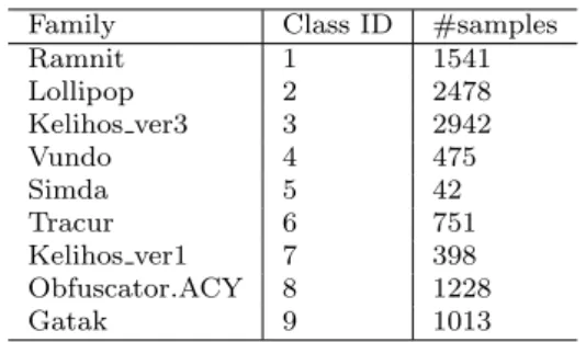
5.3 Microsoft Malware Classification Challenge Microsoft provided a dataset composed of 21741 sam-ples for the Big Data Innovators Gathering (BIG 2015) Anti-Malware Prediction Challenge, 10868 for training and 10873 for testing. Every program in the dataset has a file containing the hexadecimal representation of the malware’s binary content and its corresponding as-sembly file. However, only the label for the samples belonging to the training dataset is provided. Table 5 shows the distribution of malware programs present in the training dataset.

Table 5: BIG 2015: Distribution of Samples

Family Class ID #samples

Ramnit 1 1541 Lollipop 2 2478 Kelihos ver3 3 2942 Vundo 4 475 Simda 5 42 Tracur 6 751 Kelihos ver1 7 398 Obfuscator.ACY 8 1228 Gatak 9 1013 5.3.1 Results

Similar to the MalImg dataset, we downsampled the gray scale images. In particular, images of the BIG dataset were downsampled to 128x128 pixels because greater width and height did not improve the perfor-mance of the classifier. In addition, we performed 5-fold and 10-fold cross validation to evaluate our model. Ta-ble 6 and TaTa-ble 7 show the confusion matrices obtained for 5-fold cross validation and 10-fold cross validation.

Table 6: BIG 2015 dataset confusion matrix for 5-fold validation using images of 128x128 pixels

Family 1 2 3 4 5 6 7 8 9 Accuracy 1 1492 7 0 2 2 11 3 19 5 0.968 2 6 2424 0 1 3 10 0 3 31 0.978 3 1 0 2937 0 0 0 4 0 0 0.998 4 2 1 2 461 2 2 1 2 2 0.971 5 3 3 0 4 25 1 0 6 0 0.595 6 10 5 1 3 1 701 1 18 11 0.933 7 2 0 1 0 0 0 392 0 3 0.985 8 36 4 1 13 2 19 5 1144 4 0.932 9 2 6 0 1 0 2 2 2 998 0.985

Table 7: BIG 2015 dataset confusion matrix for 10-fold validation using images of 128x128 pixels

Family 1 2 3 4 5 6 7 8 9 Accuracy 1 1490 4 2 2 2 9 1 28 3 0.967 2 6 2440 0 0 1 7 0 8 16 0.985 3 0 1 2938 1 0 0 2 0 0 0.999 4 3 0 2 461 2 1 1 3 2 0.971 5 3 2 0 1 29 2 0 5 0 0.690 6 8 6 1 2 0 713 2 10 9 0.948 7 1 0 5 1 0 0 391 0 0 0.982 8 44 4 2 8 2 17 5 1138 8 0.923 9 2 2 0 0 0 6 2 5 996 0.983

Table 8: Performance comparison of various methods for classification of BIG 2015 training dataset. 1-nearest neighbor (1-NN). Support vector machines (SVM). Static feed-forward network (SFN1 & SFN2). Dynamic feed-forward network (DFN)

Method 5-fold accuracy Macro-averaged

F1 Score Haralick features + XGBoost 0.955

-LBP features + XGBoost 0.951 -CNN 0.973 0.927 10-fold accuracy 12 PCA features + 1-NN 0.966 0.910 10 PCA features + SVM 0.946 0.864 52 PCA features + SFN1 0.956 0.884 52 PCA features + SFN2 0.942 0.849 52 PCA features + DFN 0.955 0.889 CNN 0.975 0.940

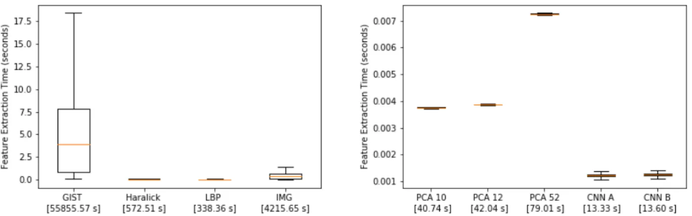
Table 8 presents the results obtained by state-of-the-art approaches in the literature that had extracted image-based features to classify malware from the BIG dataset. To sum up, Narayanan et al. [18] used PCA to extract the first 10, 12 and 52 principal components and classify malware using different machine learning classification algorithms. Moreover, Ahmadi et al. [1] extracted Haralick and local binary pattern features from images and trained an ensemble of trees for classi-fication. Their approaches were evaluated using 5-fold and 10-fold cross validation, respectively. As can be ob-served, our method outperformed the rest of approaches in the literature, achieving 0.973 and 0.975 accuracy, for 5-fold and 10-fold cross validation, respectively. Fur-thermore, the average classification time of our approach is 0,001 seconds. Fig. 6 shows the computational time of every feature extraction method evaluated. The im-provement of our method is equal to 99.98%, 98.47%

Fig. 6: The required time of feature extraction from the grayscale representation for each program. The time in brackets shows the total time of extraction for all training samples. LBP stands for local binary patterns. IMG denotes how much time it takes to transform a binary executable into a gray-scale image. PCA 10, PCA 12 and PCA 52 refer to the number of principal components used. CNN A refers to the time needed to extract the features by the convolutional network and CNN B refers to the time the networks needs to extract features and classify a sample.

and 96.06% with respect to the computational time needed to extract GIST, Haralick and local binary pat-tern features. Additionally, our method is 67.35%, 68.29% and 83.13% faster than the calculation of the 10, 12 and 52 principal components.

6 Conclusions

This paper presents a novel file agnostic deep learn-ing system for classification of malware based on its visualization as gray-scale images. As far as we know, it is the first approach to apply deep learning to find patterns from malware’s binary content represented as images. The proposed solution has a number of advan-tages that allow malicious programs to be detected in a real-time environment. Firstly, it is file agnostic and is based solely on the binary code of an executable. Sec-ondly, the transformation of an executable into a gray-scale image is inexpensive. Thirdly, the prediction time is minimal. Fourthly, it obtained greater classification accuracy than all previous methods in the literature that were based on the representation of malware as gray-scale images.

6.1 Limitations and Future Work

Despite the fact that our approach was able to outper-form state-of-the-art methods in terms of accuracy and classification time, it has some issues that are directly

related to the visualization of malware as grayscale im-ages. Even though it can be seen that the visualiza-tion of malware programs belonging to the same family has similar patterns, this approach has problems with some samples that have been compressed or encrypted, which may have a completely different overall structure. For instance, the visualization of samples from the Au-torun.K and Yuner.A families are almost equal. To deal with such cases, we suggest combining the features ex-tracted by the convolutional neural network with hand-designed features as input of a machine learning model based on distinct types of file features [1].

Acknowledgements We would like to thank the Blueliv Labs team, especially Daniel Sol´ıs, and `Angel Puigvent´os for their support and the feedback provided during the develop-ment of this work. This work has been partially funded by the Spanish MICINN Projects TIN2014-53234-C2-2-R, TIN2015-71799-C2-2-P and by AGAUR DI-2016-091.

Conflict of Interest: The authors declare that they have no conflict of interest.

References

1. Ahmadi, M., Giacinto, G., Ulyanov, D., Semenov, S., Trofimov, M.: Novel feature extraction, selection and fu-sion for effective malware family classification. CoRR

abs/1511.04317(2015)

2. Anderson, B., Quist, D., Neil, J., Storlie, C., Lane, T.: Graph-based malware detection using dynamic analysis. J. Comput. Virol. 7(4), 247– 258 (2011). DOI 10.1007/s11416-011-0152-x. URL http://dx.doi.org/10.1007/s11416-011-0152-x

3. Bat-Erdene, M., Park, H., Li, H., Lee, H., Choi, M.S.: En-tropy analysis to classify unknown packing algorithms for malware detection. International Journal of Information Security16(3), 227–248 (2017)

4. Billar, D.: Opcodes as predictor for malware. Interna-tional Journal of Electronic Security and Digital Foren-sics1, 156––168 (2007)

5. Chandrasekar Ravi, R.M.: Malware detection using win-dows api sequence and machine learning. International Journal of Computer Applications43(2012)

6. Egele, M., Scholte, T., Kirda, E., Kruegel, C.: A survey on automated dynamic malware-analysis tech-niques and tools. ACM Comput. Surv. 44(2), 6:1– 6:42 (2008). DOI 10.1145/2089125.2089126. URL http://doi.acm.org/10.1145/2089125.2089126

7. Gandotra, E., Bansal, D., Sofat, S.: Malware analysis and classification: A survey. Journal of Information Security pp. 56–64 (2014)

8. Ghiasi, M., Sami, A., Salehi, Z.: Dynamic vsa: a frame-work for malware detection based on register contents. Engineering Applications of Artificial Intelligence 44, 111–122 (2015)

9. Han, K.S., Lim, J.H., Kang, B., Im, E.G.: Malware anal-ysis using visualized images and entropy graphs. Interna-tional Journal of Information Security14(1), 1–14 (2015) 10. Haralick, R.M., Shanmugam, K., Dinstein, I.: Textural Features for Image Classification. IEEE Transactions on Systems, Man, and CyberneticsSMC-3(6), 610–621 (1973)

11. Hotelling, H.: Analysis of a complex of statistical vari-ables into principal components. J. Educ. Psych. 24

(1933)

12. Hubel, D.H., Wiesel, T.N.: Receptive fields and func-tional architecture of monkey striate cortex. Journal of Physiology (London)195, 215–243 (1968)

13. Krizhevsky, A., Sutskever, I., Hinton, G.E.: Imagenet classification with deep convolutional neural networks. In: Proceedings of the 25th International Conference on Neural Information Processing Systems, NIPS’12, pp. 1097–1105. Curran Associates Inc., USA (2012)

14. Lecun, Y., Bottou, L., Bengio, Y., Haffner, P.: Gradient-based learning applied to document recognition. In: Pro-ceedings of the IEEE, pp. 2278–2324 (1998)

15. LLC, M.: Mcafee labs threats report (2017)

16. Lyda, R., Hamrock, J.: Using entropy analysis to find en-crypted and packed malware. IEEE Security and Analy-sis5, 40–45 (2007)

17. Nair, V., Hinton, G.E.: Rectified linear units improve re-stricted boltzmann machines. In: Proceedings of the 27th International Conference on International Conference on Machine Learning, ICML’10, pp. 807–814. Omnipress, USA (2010)

18. Narayanan, B.N., Djaneye-Boundjou, O., Kebede, T.M.: Performance analysis of machine learning and pattern recognition algorithms for malware classification. In: Aerospace and Electronics Conference (NAECON) and Ohio Innovation Summit (OIS), 2016 IEEE National, pp. 338–342. IEEE (2016)

19. Nataraj, L., Karthikeyan, S., Jacob, G., Manjunath, B.S.: Malware images: Visualization and automatic classifica-tion. In: Proceedings of the 8th International Symposium on Visualization for Cyber Security, VizSec ’11, pp. 4:1– 4:7. ACM, New York, NY, USA (2011)

20. Ojala, T., Pietikainen, M., Harwood, D.: Performance evaluation of texture measures with classification based on Kullback discrimination of distributions. In: Pattern

Recognition, 1994. Vol. 1 - Conference A: Computer Vi-sion amp; Image Processing., Proceedings of the 12th IAPR International Conference on, vol. 1 (1994) 21. Oliva, A., Torralba, A.: Modeling the shape of the scene:

A holistic representation of the spatial envelope. Int. J. Comput. Vision42(3), 145–175 (2001)

22. Ranvee, S., Hiray, S.: Comparative analysis of feature extraction methods of malware detection. International Journal of Computer Applications120(2015)

23. Salehi, Z., Sami, A., Ghiasi, M.: Maar: Robust features to detect malicious activity based on api calls, their ar-guments and return values. Engineering Applications of Artificial Intelligence59, 93–102 (2017)

24. Shabtai, A., Moskovitch, R., Feher, C., Dolev, S., Elovici, Y.: Detecting unknown malicious code by applying clas-sification techniques on opcode patterns. In: Security Informatics. Springer (2012)

25. Sorokin, I.: Comparing files using structural entropy. Journal in Computer Virology7(4), 259 (2011)

26. Srivastava, N., Hinton, G., Krizhevsky, A., Sutskever, I., Salakhutdinov, R.: Dropout: A simple way to prevent neural networks from overfitting. Journal of Machine Learning Research15, 1929–1958 (2014)

27. Storlie, C., Anderson, B., Vander Wiel, S., Quist, D., Hash, C., Brown, N.: Stochastic identification of malware with dynamic traces. Ann. Appl. Stat.

8(1), 1–18 (2014). DOI 10.1214/13-AOAS703. URL https://doi.org/10.1214/13-AOAS703

28. Tesauro, G., Kephart, J., Sorkin, G.B.: Neural networks for computer virus recognition. IEEE International Conference on Intelligence and Security Informatics11

(1996)

29. Yuxin, D., Siyi, Z.: Malware detection based on deep learning algorithm. Neural Computing and Applications (2017)