San Jose State University
SJSU ScholarWorks
Master's Projects Master's Theses and Graduate Research
Fall 2013
Hidden Markov Models for Malware Classification
Chinmayee Annachhatre
San Jose State UniversityFollow this and additional works at:https://scholarworks.sjsu.edu/etd_projects Part of theComputer Sciences Commons
This Master's Project is brought to you for free and open access by the Master's Theses and Graduate Research at SJSU ScholarWorks. It has been accepted for inclusion in Master's Projects by an authorized administrator of SJSU ScholarWorks. For more information, please contact
Recommended Citation
Annachhatre, Chinmayee, "Hidden Markov Models for Malware Classification" (2013).Master's Projects. 328. DOI: https://doi.org/10.31979/etd.t5hr-x8s9
Hidden Markov Models for Malware Classification
A Project Presented to
The Faculty of the Department of Computer Science San Jose State University
In Partial Fulfillment
of the Requirements for the Degree Master of Science
by
Chinmayee Annachhatre December 2013
c
2013
Chinmayee Annachhatre ALL RIGHTS RESERVED
The Designated Project Committee Approves the Project Titled
Hidden Markov Models for Malware Classification
by
Chinmayee Annachhatre
APPROVED FOR THE DEPARTMENTS OF COMPUTER SCIENCE
SAN JOSE STATE UNIVERSITY
December 2013
Dr. Mark Stamp Department of Computer Science Dr. Chris Pollett Department of Computer Science Dr. Tom Austin Department of Computer Science
ABSTRACT
Hidden Markov Models for Malware Classification by Chinmayee Annachhatre
Malware is a software which is developed for malicious intent. Malware is a rapidly evolving threat to the computing community. Although many techniques for malware classification have been proposed, there is still the lack of a comprehensible and useful taxonomy to classify malware samples.
Previous research has shown that hidden Markov model (HMM) analysis is useful for detecting certain types of malware. In this research, we consider the related problem of malware classification based on HMMs. We train HMMs for a variety of malware generators and a variety of compilers. More than 9000 malware samples are then scored against each of these models and the malware samples are separated into clusters based on the resulting scores. We analyze the clusters and show that they correspond to certain characteristics of malware. These results indicate that HMMs are an effective tool for the challenging task of automatically classifying malware.
ACKNOWLEDGMENTS
I would like to express my gratitude to my project advisor, Dr. Mark Stamp for his encouragement, guidance and support throughout my graduate studies. He has always been patient in listening to the little issues and roadblocks that came up while working on the project. He was of great help in requesting the dataset from the Malicia project group, without which the project’s successful completion was not possible.
I would also like to thank my committee member Dr. Chris Pollett for his time and guidance.
A very special thanks to my committee member, Dr. Tom Austin for his valu-able inputs and also the dataset that he provided for the assembly generated by the compilers and the hand-written assembly.
Finally, I would also like to thank my husband, Mr. Vivek Rane for his persistent support and guidance throughout my Masters.
TABLE OF CONTENTS
CHAPTER
1 Introduction . . . 1
2 Malware and Detection Techniques . . . 4
2.1 Malware . . . 4
2.1.1 Virus . . . 5
2.1.2 Worm . . . 7
2.1.3 Trojan . . . 7
2.1.4 Trapdoor/Backdoor . . . 8
2.2 Malware Detection Techniques . . . 8
2.2.1 Signature Based Detection . . . 8
2.2.2 Anomaly Based Detection . . . 9
2.2.3 Hidden Markov Model Based Detection . . . 9
3 Related Work . . . 15
3.1 Classification of Malware using Structured Control Flow . . . 15
3.2 Behavioral Malware Classification . . . 15
3.3 Malware Classification using the data mining methods . . . 17
3.3.1 Instance-based Learner . . . 17
3.3.2 Support Vector Machines (SVM) . . . 18
3.3.3 Na¨ıve Bayes . . . 18
3.3.4 Decision Trees . . . 18
3.4 VILO: A Rapid Learning Nearest-Neighbor Classifier for Malware
Classification . . . 19
4 Clustering Algorithms . . . 21
4.1 k-means Clustering Algorithm . . . 22
4.1.1 Advantages of the k-means clustering algorithm . . . 24
4.1.2 Disadvantages of the k-means clustering algorithm . . . 24
5 Implementation . . . 25
5.1 Training HMMs . . . 25
5.2 Collection of the dataset . . . 25
5.3 Scoring the dataset . . . 26
5.4 k-means Clustering Algorithm . . . 27
5.4.1 Example - Distance Calculation . . . 29
6 Experiments . . . 32
6.1 Setup . . . 32
6.2 Discussion on Results . . . 33
6.2.1 Classification and Clustering . . . 33
6.2.2 Why is clustering important? . . . 36
7 Conclusion and Future Work . . . 38
APPENDIX Graphs fork-means Clustering Algorithm for Malware Classification 44 A.1 k = 2 (Number of Clusters=2) . . . 44
A.2 k = 3 (Number of Clusters=3) . . . 45
A.4 k = 5 (Number of Clusters=5) . . . 46
A.5 k = 6 (Number of Clusters=6) . . . 46
A.6 k = 7 (Number of Clusters=7) . . . 47
A.7 k = 8 (Number of Clusters=8) . . . 47
A.8 k = 9 (Number of Clusters=9) . . . 48
A.9 k = 10 (Number of Clusters=10) . . . 48
A.10k = 2 (Number of Clusters=2) . . . 49
A.11k = 3 (Number of Clusters=3) . . . 50
A.12k = 4 (Number of Clusters=4) . . . 50
A.13k = 5 (Number of Clusters=5) . . . 51
A.14k = 6 (Number of Clusters=6) . . . 51
A.15k = 7 (Number of Clusters=7) . . . 52
A.16k = 8 (Number of Clusters=8) . . . 52
A.17k = 9 (Number of Clusters=9) . . . 53
A.18k = 10 (Number of Clusters=10) . . . 53
A.19k = 11 (Number of Clusters=11) . . . 54
A.20k = 12 (Number of Clusters=12) . . . 54
A.21k = 13 (Number of Clusters=13) . . . 55
A.22k = 14 (Number of Clusters=14) . . . 55
LIST OF TABLES
1 Count of samples used for the training of HMM . . . 26
2 Malware Samples in the dataset . . . 27
3 7-tuple of a centroid . . . 28
4 Sample record in the dataset . . . 28
5 Example of a malware sample . . . 29
6 Initial centroids . . . 30
LIST OF FIGURES 1 Malware Growth [33] . . . 4 2 Simple Virus [13] . . . 5 3 Encrypted Virus [13] . . . 6 4 Polymorphic Virus [13] . . . 6 5 Metamorphic Virus [13] . . . 7
6 A Hidden Markov Model [38] . . . 11
7 Stacked Column Chart for 9 Clusters . . . 34
CHAPTER 1 Introduction
Malicious software is called malware. Malware can steal sensitive data from a computer or it can infect files one after the other one file, then another, and spread the infection throughout the computer. Malware needs to be caught and removed from the infected computer in time to avoid the leakage of sensitive data or any other malicious activity in the computer. In recent years smartphones have started to become more popular and are one of the preferred devices for most consumers across the world. The widespread use of smartphones along with continuous internet connectivity and the “always on” paradigm makes them a lucrative target for malware attacks. Malware includes all families of viruses, computer worms, Trojans, backdoor, spyware, adware, etc. See Chapter 2 for more details. According to [43], “malware or malicious code is a rapidly evolving threat to the computing community. Zero-day malware are exploiting vulnerabilities very soon after being discovered and are spreading quickly. However, anti-virus tools, which are the most widely used countering mechanism, are unable to cope with this. They are based on signatures which need to be computed for new malware strains. After a new malware strikes and before the signature is found, there is a sufficient time for the malware to perform its damage.” Hackers fine-tune their malware against antivirus software and make their code harder to detect. Various alternative malware detection techniques are also available. These are elaborated in Chapter 2. By far, there are many techniques proposed for malware classification. However, there is still the lack of a comprehensible and useful taxonomy to classify malware samples. We have dealt with the problem of malware classification in this project.
Malware authors and distributors have been taking advantage of exploit kits in order to spread malware rapidly. By far, blackhole is the most significant and the leading exploit kit [16]. The Blackhole Exploit Kit is one of the most popular attack tools used to infect Web users with malware. Its purpose is to deliver a malicious payload to a victim’s computer. The users are redirected from compromised websites to Blackhole landing pages hosted on malicious servers to install malware on computers with vulnerable software [16].
One of the world’s most sophisticated malware worm, Stuxnet, was discovered in June 2010 targeting industrial control systems. It was created to attack Iran’s nuclear facilities. It initially spreads through Microsoft Windows and targets Siemens industrial control systems. Its main aim was to reprogram the industrial control systems in a stealthy way in order to cause damage. It utilized zero-day exploits, a Windows and a programmable logic controller (PLC) rootkit, antivirus evasion, process injection and hooking techniques, network spreading, updates using P2P and a command and control interface [45].
Koobface is a multi-platform computer worm that originally targets users of so-cial networking websites like Facebook, Skype, Twitter, hi5 etc. It gathers login information for such sites [5]. It does not collect any sensitive financial data [44]. The Koobface threat comprises several component malware files that work together to form and maintain the Koobface botnet. This threat model enables Koobface to update its existing components on an affected system, add new ones or stop updat-ing nonworkupdat-ing modules [5]. Koobface cleverly uses social networkupdat-ing sites’ internet cookies to identify what sites an affected user is a member of in order to access the user’s social network account and to send Koobface-related messages on the affected social-networking site [5].
This shows that malware is a very serious threat that is expanding rapidly day-by-day. However, there is still a lack of comprehensible and useful taxonomy to classify malware. Malware taxonomy is useful in several ways. Firstly, it can allow faster response to new threats – If the new malware can fit in the existing classification, the anti-malware detection and removal are already known. Hence, the new malware can be removed with the known techniques. If it does not fit into the existing classification, the known techniques of malware detection and removal will not work. Hence, the new techniques need to be found out [2]. Secondly, malware taxonomy helps in better understanding of malware activities. It might help us in knowing the functionality of the malware and their relationship with other malware. In this research, we attempt to resolve the problem of malware classification based on HMMs. Our technique is inspired by the approach followed in [3]. We train HMMs for a variety of malware generators and a variety of compilers. More than 9000 malware samples are then scored against each of these models and the malware samples are separated into clusters based on the resulting scores. We analyze the clusters and show that they correspond to certain characteristics of malware. These results indicate that HMMs are an effective tool for the challenging task of automatically classifying malware.
This paper is organized as follows: Chapter 2 includes definitions and information on the types of malware and different malware detection strategies. Chapter 3 gives an overview of the previous work on the malware classification. Chapter 4 explains thek-means clustering algorithm and other alternatives available. Chapter 5 includes the implementation of k-means clustering algorithm used for malware classification in detail. Chapter 6 includes the experiments and results, and the benefits of the clustering method. Chapter 7 ends with the conclusion and suggests future work.
CHAPTER 2
Malware and Detection Techniques 2.1 Malware
As mentioned in Chapter 1, malware is a software program developed to perform malicious activities on a computer. There can be any reasons for writing malware varying from simple pranks to serious organized internet crimes. The early infectious programs (also the first Internet Worm, Morris Worm) were written as pranks [30]. Now-a-days, malware is widely used to steal confidential personal, financial, business information. Figure 1 shows how the malware is rapidly increasing in volume day-by-day. The x-axis in Figure 1 indicates the year and the y-axis indicates the number of malware samples generated in the specified year on the x-axis.
Figure 1: Malware Growth [33]
As mentioned in Chapter 1, malware includes all families of viruses, computer worms, Trojans, backdoor, spyware, adware etc. A brief overview of different types of malware is given below:
2.1.1 Virus
A virus is a type of malware that replicates itself by inserting copies or modified copies of itself into other programs. They can live anywhere. It can live on the boot sector. If it lives on the boot sector, it can take control before anything else [26]. As mentioned in [4], “it establishes itself before any antivirus software starts or operating system security is enabled.” It can also live in the memory. It can enter the computer via email, internet or different types of external storage media like flash drives, floppy disks. As pointed out in [32], “They have the ability to reproduce infecting other files and programs. When they are run, they are able to carry out a range of annoying or damaging actions in your computer.” Virus writers constantly modify their software to evade the detection techniques. The prominent methods to evade the detection techniques are encryption, polymorphism and metamorphism. These are described in Figure 2.
Figure 2: Simple Virus [13]
2.1.1.1 Encrypted Virus
Antivirus software searches for a signature (a specific bit string) for virus detec-tion. The simplest method to hide the virus body (signature) is to encrypt it with different encryption keys. As a result of this, the detection of a virus becomes a difficult task. The idea of an encrypted virus is to encrypt the signature in order to evade signature detection. However, it is still possible to search for an encrypted signature too. Thus, the encrypted virus is not a reliable way of evading signature
detection. The only part that is constant in the encrypted virus is the decryptor loop. Antivirus software will exploit this fact for detection, so the next logical development is to change the decryptor loop’s code with each infection [4]. The figure 3 shows graphical representation for the encrypted virus.
Figure 3: Encrypted Virus [13]
2.1.1.2 Polymorphic Virus
The above problem of non-decrypted decryptor loop is solved in polymorphism. The decryptor loop is morphed in each generation. According to [4], “A polymorphic virus has, for all practical purposes, an infinite number of decryptor loop variations. Tremor, for example, has almost six billion possible decryptor loops! Polymorphic viruses clearly can’t be detected by listing all the possible combinations.” The tech-niques such as emulation can be used for polymorphic virus detection. Figure 4 shows graphical representation for the polymorphic virus.
Figure 4: Polymorphic Virus [13]
2.1.1.3 Metamorphic Virus
Virus writers modified the malware furthermore to avoid emulation detection. The metamorphic virus is also called as body polymorphic virus. The appearance of the virus changes before infecting any system. The detection of a metamorphic virus is very challenging. The morphed virus has the same functionality but a different
structure. Hence the detection of metamorphic virus is difficult. Figure 5 shows graphical representation for the polymorphic virus.
Figure 5: Metamorphic Virus [13]
2.1.2 Worm
A computer worm is a standalone malware computer program that replicates itself in order to spread to other computers [14]. As pointed out in [40], “worms are programs that replicate themselves from system to system without the use of a host file. This is in contrast to viruses, which requires the spreading of an infected host file.” Worms replicate themselves damaging files, but can reproduce rapidly, saturating a network and causing it to collapse. Some of the examples of the notorious worms sent via email are: Navidad, Pretty Park, Happy99, ExploreZip [32].
2.1.3 Trojan
A Trojan is a non-self-replicating type of malware which appears to perform a desirable function but instead drops a malicious payload [40]. An important difference between Trojan and a virus is that the Trojan does not replicate itself [40]. They pose as legitimate programs that users may recognize and want to use [41]. When these are executed, they install other programs on the computer which can be harmful [32]. The Trojans have the capacity of deleting files, destroying information on the hard drive, or open a backdoor to the security systems [32]. Some examples of Trojans are Backdoor, Crack2000, KillCMOS and BetBus [32].
2.1.4 Trapdoor/Backdoor
A trapdoor/backdoor is a program which bypasses the security check [4]. This allows a malicious user to carry out actions on the affected computer that can com-promise user confidentiality or impede the operations carried out [32]. The actions that backdoor allow malicious users to carry out can be extremely damaging. They could allow them to delete files or destroy all the information on the hard disk, cap-ture confidential data and send it out to an external address or open communications ports, allowing remote control of the computer. Some examples of backdoor are: Orifice2K.sfx, Bionet.318, Antilam y Subseven.213 [32].
We have not used these families as the target categories for our classification of malware. The reason for this is that if an unknown malware is classified into these families, the detection and removal strategies for that particular malware will be not known, since this classification is too generalized. Even if there are detection and removal strategies for these families, there is no way of determining this information. Instead, we used the information for malware family types provided in the dataset.
2.2 Malware Detection Techniques
As malware writers fine-tune their software by making it better to evade signa-ture detection, the anitivirus companies are improving their detection techniques as well. The following sections describe the signature based detection, anomaly based detection and hidden Markov model based detection strategies.
2.2.1 Signature Based Detection
Signature based detection is a simple and most commonly used technique in antivirus software. They are popular because of accurate detection, simplicity and
speed [37]. In signature based detection, the scanner scans each executable and looks for specific string or pattern of bits (signatures). Antivirus software has a database of signatures for different viruses. By comparing the signature, it detects the virus. The disadvantage is that only the known malware can be detected. If the signature is not unknown, malware cannot be detected. The signature file must be kept up to date. By using simple code obfuscation techniques, malware can easily evade the signature based detection [34].
2.2.2 Anomaly Based Detection
The problem of detecting new malwares in signature based detection can be overcome using anomaly based detection. Heuristic methods are implemented to detect anomalous behavior. This technique comprises of two phases - the training phase and the detection phase. In the training phase, the model is trained with the normal behavior. Anything other than the normal behavior is considered as malicious behavior [17]. However, there can be more false positives in this technique [37].
2.2.3 Hidden Markov Model Based Detection
Hidden Markov models (HMMs) are generally used for statistical pattern anal-ysis. They can be used in speech recognition, malware detection [35] and biological sequence analysis [24]. The following sections give an overview of the introduction to HMM and its usage in detection of malware.
2.2.3.1 Introduction to HMM
A statistical model that has states and known probabilities of the state transitions is called a Markov model [38]. In such a Markov model, the states are visible to
the observer. In contrast, a hidden Markov model (HMM) has states that are not directly observable [35]. HMM is a machine learning technique. HMM acts as a state machine. Every state is associated with a probability distribution for observing a set of observation symbols. The transition between the states have fixed probabilities. We can train an HMM using the observation sequences to represent a set of data [38]. We can match an observation sequence against a trained HMM to determine the probability of seeing such a sequence. If the probability is high, the observation sequence is similar to the training sequences. HMMs are used in protein modeling [24]. HMM can also be used to detect certain types of software piracy detection [22]. As mentioned in [38], the following table shows the notations used in the hidden Markov models:
T = length of the observation sequence
N = number of states in the model
M = number of distinct observation symbols
Q= distinct states of the Markov Model
V = set of possible observations
A= state transition probability matrix
B = observation probability matrix
π = initial state distribution
O = observation sequence
A hidden Markov model is defined by the matrices A, B and π. An HMM is denoted as λ = (A, B, π). Figure 6 represents a generic view of a hidden Markov model.
Markov process: X0 A - X1 A - X2 A - · · · A - XT−1 ? B ? B ? B ? B Observations: O0 O1 O2 · · · OT−1 Figure 6: A Hidden Markov Model [38]
Problem 1: Given a model λ = (A, B, π) and an observation sequence O, we need to findP(O|λ). That is, an observation sequence that can be scored to see how well it fits a given model [38].
Problem 2: Given a model λ = (A, B, π) and an observation sequence O, we can determine an optimal state sequence for the Markov model. That is, the most likely hidden state sequence can be uncovered [38].
Problem 3: GivenO,N, M, we can find a modelλ that maximizes probability ofO. This is the training of a model in order to best fit an observation sequence [38]. In this project, the algorithms for Problems 1 and 3 are used. First we train an HMM to represent a set of data, which is in the form of observation sequences. We have trained the models using a variety of compilers and malware generators. This is equivalent to using the algorithm for Problem 3. Then the resulting HMM can be used to score the malware samples against the model. This is equivalent to using the algorithm for Problem 1. These three problems can be efficiently solved by the following three algorithms:
• The Forward algorithm.
• The Baum-Welch reestimation algorithm.
The forward-backward algorithm is for calculating the probability of being in a state
qi at time t given an observation sequenceO [38]. The forward algorithm, or α pass,
determines P(O|λ) [38]. The algorithm can be stated as follows.
1. For t = 0,1, . . . , T −1 andi= 0,1, . . . , N −1 2. αt(i) = P(O0,O1, . . . ,Ot, xt=qi|λ)
The probability of the partial observation sequence up to time t is αt(i). Using the
forward algorithm, P(O|λ) can be computed as follows [38].
1. Let α0(i) = πibi(O0), fori= 0,1, . . . , N −1
2. For t = 1,2, . . . , T −1 andi= 0,1, . . . , N −1 compute
αt(i) = N−1 X j=1 αt−1(j)aij)bi(Ot) 3. Then P(O|λ) = (PN−1 i=0 αT−1(i)
The backward algorithm helps to find a most likely optimal state sequence. This algorithm can be stated as follows [38].
1. For t = 0,1, . . . , T −1 andi= 0,1, . . . , N −1 define 2. βt(i) =P(Ot+1,Ot+2, . . . ,OT−1, xt=qi, λ)
Then βt(i) can be calculated in following steps [38]:
2. For t =T −2, T −3, . . . ,0 and i= 0,1, . . . , N −1, compute βt(i) = N−1 X j=0 aijbj(Ot+1)βt+1(j)
Fort = 0,1, . . . , T −2 andi= 0,1, . . . , N −1 define
γt(i) =P(xt=qi|O, λ)
The relevant probability up to time t is given by [38],
γt(i) =
αt(i)βt(i)
P(O|λ)
The most likely state at any time t is the state for which γt(i) is maximum. The
Baum-Welch algorithm helps in iteratively re-estimating the parametersA,B,π [38]. It provides efficient way to best fit the observations. The number of states N and number of unique observation symbols M are constant. However, other parameters like A, B and π are changeable with row stochastic condition. This process of re-estimating the model is explained as follows [38]:
1. Initialize λ= (A, B, π) with an appropriate guess or random values. For exam-ple π = 1/N, Aij = 1/N, Bij = 1/M.
2. Compute αt(i), βt(i), γt(i) and γt(i, j) where γt(i, j) is a gamma. The
di-gammas can be defined as:
γt(i) =
αt(i)aijbj(Ot+1)βt+1(j)
P(O|λ)
γt(i) and γt(i, j) are related by:
γt(i) = N−1 X
j=0
3. Re-estimate model parameters as: For i= 0,1, . . . , N −1 let
πi =γ0(i)
Fori= 0,1, . . . , N −1 andj = 0,1, . . . , N −1, compute
aij = T−2 P t=0 γt(i, j) T−2 P t=0 γt(i)
Forj = 0,1, . . . , N −1 and k= 0,1, . . . , M −1, compute
bj(k) = P t0,1,...,T−1,Ot=k γt(j) T−2 P t=0 γt(j) 4. If P(O|λ) increases go to step 3.
2.2.3.2 HMM For Malware Detection
When an HMM is trained, it can be used to distinguish between a malware and a benign file [38, 47]. There is a lot of previous work done on the use of HMM for malware detection. The dataset is tested against the trained models. There is a range of values of scores for which the scores of the malware and the benign files do not overlap [36]. This is known as threshold. Using this threshold, the malware can be distinguished from the benign files [47].
CHAPTER 3 Related Work
A lot of previous work is done on detection and classification of malware. This chapter discusses some attempts made for malware classification, which include usage of structured control workflow and some other data mining methods.
3.1 Classification of Malware using Structured Control Flow
Control flow represents the execution path a program may take. Control flow information appears in two main forms. The call graph represents the inter-procedural control flow. The intra-procedural control flow is represented as a set of control flow graphs with one graph per procedure [9]. In [9], the research has shown that malware can be effectively be characterized by its control flow. The authors have proposed a malware classification system using approximate matching of control flow graphs. The string edit distances can be calculated between the control flow signatures and the structured graphs of the malware in the database. The threshold is decided. If the edit distance exceeds a particular threshold, then the binary can be classified as a malicious binary, else it is a benign binary. Control flow is more invariant among polymorphic and metamorphic malware. The research shows that the proposed method could successfully identify variants of malware [9].
3.2 Behavioral Malware Classification
Classification systems generally fall into one of two categories: Those that rely on features extracted from static files, or those that execute malware and use behav-ioral features to classify malware. Static approaches sometimes use low-level features
such as calls to external libraries, strings, and byte sequences for classification [23]. Other static approaches extract more detailed information from binaries, including sequences of API calls, the graphical representations of control flow [9]. Although the many variants in a malware family have different static signatures, they share char-acteristic behavioral patterns resulting from their common function and heritage [8]. The authors in [8] have described a automatic classification system that can be trained to accurately identify new variants within known malware families, using observed similarities in behavioral features extracted from sensors monitoring live computer hosts. In the feature selection used in [8], the authors have selected a set of observ-able features that are easily extracted from live computer hosts, and whose values can be used to infer whether a detected malware sample belongs to particular category or family. The authors have considered the following features: the data collected from performance monitors that report resource usage, the frequency of calls to specific kernel functions, and the frequency of calls to specific sequences of kernel functions. The system proposed by authors uses decision trees for classification, which label each newly detected malware sample as one of the existing labels learned during training. If a new malware sample does not belong to one of the existing labels, the decision trees simply label it (incorrectly) with one of the existing labels. To address the issue of new malware samples that are not well-described by an existing label, the authors have used other types of classifiers. They have explored the use of the nearest centroid algorithm [49], which can be used to establish a notion of distance from the centroids that define the labels. If the malware whose distance to the closest centroid exceeded a threshold, it might be considered new malware that required further analysis. The authors used k-means clustering algorithm [7] to deal with the behavioral diversity of malware having a particular label to establish multiple centroids for characterizing each malware label and also exploring the use of subfamily labels for classification.
The presented results indicate that the behavioral classifier can correctly identify new malware variants within certain families of malware.
3.3 Malware Classification using the data mining methods
In [23], the authors have extracted the byte sequences from the executables, converting these into n-grams, and constructed several classifiers: instance-based learner, Na¨ıve Bayes, decision trees, support vector machines and boosting. They viewed each n-grams as a Boolean attribute that is either present in (i.e., T) or absent from (i.e., F) the executable. They have shown that the boosted decision trees outperformed the other methods. The following section shows the methods used in their research.
3.3.1 Instance-based Learner
One of the simplest learning methods is the instance-based (IB) learner [1]. Its concept description is a collection of training examples or instances. Learning, there-fore, is the addition of new examples to the collection. An example is found in the collection that is most similar to the unknown and the examples class label is returned as its prediction for the unknown. The authors have used the number of values the two instances have in common as the measure of similarity. In the variation of this method, such as IBk, the k most similar instances are found and the majority vote of their class labels is returned as the prediction. Values for k are typically odd to prevent ties [23]. These are also called as nearest neighbor and k-nearest neighbors.
3.3.2 Support Vector Machines (SVM)
Support Vector Machines [12] are supervised learning models with associated learning algorithms that analyze data and recognize patterns, used for classification. In [23], the authors produce a linear classifier, so its concept description is a vector of weights, w~ and a threshold, b. SVMs use a kernel function to map training data into a higher-dimensioned space so that the problem is linearly separable. In a high-dimensional space, a hyperplane is built and used for classification. The method predicts the positive class ifw.~~ x−b >0 and predicts the negative class otherwise [23]. ~x
is the set of points on the hyperplane. Thus, given a set of training examples belonging to one of the two categories, an SVM assigns new examples into one category or the other.
3.3.3 Na¨ıve Bayes
Na¨ıve Bayes is a probabilistic method that has a long history in information retrieval and text classification [29]. It stores as its concept description the prior probability of each class, P(Ci), and the conditional probability of each attribute
value given the class,P(vj|Ci). These quantities are estimated by counting in training
data the frequency of occurrence of the classes and the attribute values for each class. The Bayes rule is used to compute the posterior probability of each class given an unknown instance, returning as its prediction the class with highest such value [23].
3.3.4 Decision Trees
The decision trees are built based on the training data. The internal nodes of a decision tree correspond to attributes and leaf nodes correspond to class labels. The performance element uses the attributes and their values of an instance to traverse the
tree from the root to a leaf. It predicts the class label of the leaf node [23]. It creates a node, branches, and children for the attribute and its values, removes the attribute from further consideration, and distributes the examples to the appropriate child node. This process repeats recursively until a node contains examples of the same class, at which point, it stores the class label [23]. In an effort to reduce over training, most implementations also prune induced decision trees by removing subtrees that are likely to perform poorly on test data [23]. The malware classification based on the decision trees is very fast and also accurate. The disadvantage of the decision trees is that an error in higher level of the tree may cause an error in the lower part of the tree [48].
3.3.5 Boosted Classifiers
Boosting [15] is a method for combining multiple classifiers. A set of weighted models are produced by iteratively learning a model from a weighted dataset. The generated model is then evaluated. The dataset is reweighted based upon the model’s performance [23]. The authors have provided a method of detecting unknown mali-cious code in executables using machine learning. They have extracted byte sequences from the executables, converted these into n-grams, and constructed several classi-fiers: na¨ıve Bayes, boosted SVMs and boosted decision trees. The results of their experiments have shown that the boosted decision trees outperformed other methods and achieved a true-positive rate of 0.98 and a false-positive rate of 0.05.
3.4 VILO: A Rapid Learning Nearest-Neighbor Classifier for Malware Classification
There are two different types of malware classification possible: binary and famil-ial: In the binary malware classification problem, an unknown executable is classified
as either being malicious or benign. Conversely, in the familial malware classification problem, a malicious executable is classified as belonging to a particular group of mal-ware [25]. In [25], the work is based upon the familial malmal-ware classification. VILO makes use of three components: N-perm feature vectors, Term Frequency X Inverse Document Frequency (TFIDF) weighting of features [20], and the nearest-neighbor algorithm. N-perms are obtained by sliding a window of sizen over bytes, opcodes of
n-grams. They are robust against some code obfuscations such as instruction reorder-ing [11]. VILO implements a nearest neighbor algorithm with similarities computed over TFIDF weighted opcode mnemonic permutation features (N-perms). The results in [25] showed that VILO is a quick and efficacious learner of real-world malware. TFIDF weighting of features ensures that features that are common across many types of executables are not overly emphasized [25]. This is suitable for constantly changing malware population. Nearest neighbor search does not require construction of a classification model and hence is very simple and effective [25]. The authors have also stated that VILO is not suitable for binary malware classification.
CHAPTER 4 Clustering Algorithms
Clustering is the process of classifying objects into subsets based on similarity in the context of a particular problem. The objects are thereby organized into a representation that characterizes the collection being sampled. The following section discusses the different methods of clustering [19].
• Exclusive versus non-exclusive: An exclusive classification is a partition of the set of objects. Each object belongs to exactly one subset, or cluster. Non-exclusive classification, also called overlapping classification, is the alternative in which an object can be assigned to several clusters [19].
• Intrinsic versus extrinsic: Depending on whether category labels are present on the objects being classified, there are two types (intrinsic and extrinsic clas-sification). Intrinsic classification only uses a proximity matrix to perform the classification. Intrinsic classification is called “unsupervised learning” because no labels are used for classifying the object [19]. Extrinsic classification uti-lizes category labels on the object [19]. Extrinsic classification is also called “supervised learning.”
• Hierarchical versus Partitional: Hierarchical clustering algorithms break up the data into a hierarchy of clusters, whereas partitional algorithms divide the data set into mutually disjoint partitions [18]. Hierarchical clustering algo-rithms produce a hierarchy of clusters called as a dendrogram either by merging smaller clusters into larger ones or dividing larger clusters to smaller ones [18]. Hierarchical clustering algorithms are further divided into following two types:
– Agglomerative: Initially, each point is considered as a cluster in itself. The two “nearest” clusters clusters are combined into one cluster repeatedly until all the clusters are merged into a single cluster . This is a “bottom up” approach.
– Divisive: All observations start in one cluster, and splits are performed re-cursively as one moves down the hierarchy. This is a “top down” approach. Partitional clustering algorithms generate various partitions and then evaluate them by some criterion [18]. They are also called non-hierarchical as each data point is placed in exactly one of k mutually exclusive clusters. One of the most popular partitional clustering algorithms is the k-means clustering algorithm. The number of clusterskis pre-determined. The algorithm initializes the centroids for k partitions, and then assigns each member to a cluster based on its distance from each of the centroids. It then recalculates the centroids based on newly the formed clusters. The process is repeated until the difference between the initial and the recalculated centroids is negligible.
There are key differences between hierarchical and partitional clustering [18]: 1. Partitional clustering is faster than hierarchical clustering.
2. Hierarchical clustering requires only a similarity measure, whereas the par-titional clustering requires the initial centroids/centers and the number of clusters as well.
4.1 k-means Clustering Algorithm
In this project, the k-means clustering algorithm is used for malware classifica-tion. This algorithm is one of the simplest unsupervised learning algorithms that
solves the clustering problem [27]. It classifies the dataset into a certain number of clusters (say, k), which is pre-determined. k centroids are defined at initialization, one for each cluster. These centroids may be placed as far as possible from each other. Once this initialization is complete, each data point in the dataset is associated with the centroid “nearest” to it and placed in the corresponding cluster. In the next step, the centroids for each cluster are recalculated depending on the data points that have been assigned to it. These two steps are repeated until the centroids no longer change, or until the distance between the initial centroids and the recalculated centroids is negligible. The Euclidean distance formula is used for the distances calculation. The algorithm used for this project can be described in 7 steps as shown below. Steps 1 and 2 comprise of the pre-work. Step 3 is the initialization step. Steps 4, 5 and 6 are the looping steps. Step 6 is the analysis step.
1. Collect the malware dataset.
2. Identify the number of clusters (k).
3. Initialize thek centroids (k-means) for the data, say, c1,c2, . . . , ck. This can be
done in several ways, such as random or uniform distribution on each dimension of the centroid or by simply selecting one of the data points as a centroid. 4. Determine the distance of each malware from each centroid using Euclidean
distance, and assign each malware to the cluster with the centroid closest to it. 5. Recalculate the centroids for each cluster.
6. Repeat the steps 4 and 5 until there is no (or negligible) change in cluster centroids.
7. If the formed clusters do not look reasonable, repeat steps 1-6 for different number of clusters (differentk).
4.1.1 Advantages of the k-means clustering algorithm
The k-means clustering algorithm is simple to implement. Since the distance of a point from a centroid does not depend on the distance of any other point from any centroid, these calculations can be done in parallel, thus increasing the overall speed of execution. Following are the other advantages of k-means clustering algorithm:
1. It is a simple and intuitive clustering algorithm. 2. This algorithm works well for globular clusters.
4.1.2 Disadvantages of the k-means clustering algorithm
Although k-means clustering algorithm is simple and fast and produces tighter clusters than hierarchical clustering, it has some limitations. Following are the limi-tations of k-means clustering algorithm:
1. The number of clusters k is required to be specified at the beginning. If thisk
is incorrectly guessed, the clusters may not reflect the natural classification of the data at hand.
2. Different initial values of centroids may produce different clusters. It may there-fore be necessary to try clustering with different random initializations for clus-ter centroids.
CHAPTER 5 Implementation
This chapter comprises of all the implementation details of the project. The first section gives information on training HMMs. The second section contains a brief overview of how the data was collected. The third section gives details about scoring the dataset. The fifth section is about the implementation of k-means clustering algorithm in this project.
5.1 Training HMMs
The hidden Markov models were created for four different compilers (GCC, MinGW, TurboC, Clang), hand-written assembly (TASM), virus construction kit (NGVCK) and for metamorphic code (MWOR). For each of these models, the whole dataset was divided into 5 subsets. As mentioned in [36], 4 datasets are used for training and the fifth subset is used to test the trained HMM model. This process is repeated varying the number of states from 2 to 6. The training is done for 800 iterations and models are built. This method is known as five-fold cross-validation. The number of assembly files used in each case is as shown in Table 1.
5.2 Collection of the dataset
Malware datasets are not easily available and this project requires a very sub-stantial number of malware samples. The dataset was requested from the Malicia project website [31]. It comprises of 11000+ malware binaries collected from 500 drive-by download servers over a period of 11-months [31]. We have used 9442 mal-ware samples from this dataset for malmal-ware classification. The malmal-ware samples are
Table 1: Count of samples used for the training of HMM Type Count GCC 75 Clang 72 TurboC 64 MinGW 72 MWOR 100 NGVCK 50 TASM 56
of EXE or DLL format. These are disassembled using the objdump command. Af-ter disassembling, these files are used for scoring against the HMMs implemented in 5.1. In addition to the malware binaries, the data that we received also contained a MySQL database with metadata that included information on when the malware was collected, where the malware was collected from and the classification of the malware. This database helped us realize that the clusters (after classification of the dataset into clusters using k-means clustering algorithm) actually correspond to certain characteristics of the malware.
5.3 Scoring the dataset
After training, a model should assign high probabilities to files similar to the training dataset and low probabilities to all other files. We computed the log likelihood of the malware samples. Log likelihood is strongly length dependent, since it is a sum of log transition probabilities and log observation probabilities. A longer sequence will naturally have more transitions and more observations and thus a greater log likelihood, independent of how similar it is to the training sequences. Because the sequences in the dataset may have different lengths, we divided the log likelihood of a sequence by the sequence length (which is the number of opcodes) to obtain the log
likelihood per opcode (LLPO), which adjusts for the length difference. This LLPO is the score of the sequence [47]. Since we used five-fold cross validation during the training phase, we have 25 models each for the 4 compilers (GCC, MINGW, CLANG and TURBOC), the hand-written assembly code (TASM), the metamorphic worm (MWOR) and the virus construction kit (NGVCK). Each malware sample is scored against each of the 25 models in every case and then the average score of all the 25 models is taken as the final score for that particular case.
5.4 k-means Clustering Algorithm
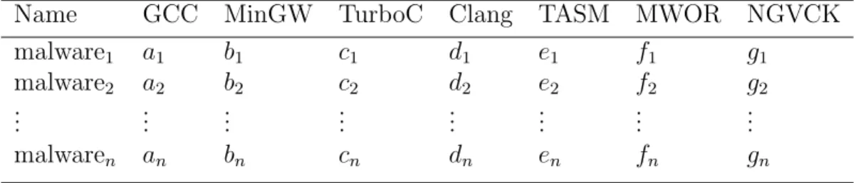
Each malware sample is represented as a 7-tuple, where each dimension represents its score generated by the specific HMM. Suppose the dataset contains n malware samples, say malware1, malware2,. . .,malwaren. The corresponding 7-tuples for these
malware samples can be shown as in Table 2.
Table 2: Malware Samples in the dataset
Name GCC MinGW TurboC Clang TASM MWOR NGVCK malware1 a1 b1 c1 d1 e1 f1 g1
malware2 a2 b2 c2 d2 e2 f2 g2
..
. ... ... ... ... ... ... ... malwaren an bn cn dn en fn gn
In Table 2,a1,a2,. . .,ancorrespond to the GCC scores,b1,b2,. . .,bncorrespond
to the MinGW scores, c1, c2, . . ., cn correspond to the TurboC scores, d1, d2, . . ., dn
are the Clang scores ofnmalware samples, e1,e2,. . .,en are the TASM scores,f1,f2,
. . .,fn are the MWOR scores and g1, g2,. . ., gn correspond to the NGVCK scores.
The range of each dimension of the dataset is divided into k parts. Since all the malware samples in a cluster are 7-tuples (7-dimensional), the centroid for each
cluster is also a 7-tuple. For every cluster, the mean is computed for each dimension. Table 3 represents the centroid, i.e., the 7-tuple with the mean values thus computed. The mean of scores in the first dimension of the first cluster is given by:
amean =
(a1 +a2+....+an/k)
n/k
Similarly, means for all the other dimensions are calculated. The resulting 7-tuple is considered the centroid for that corresponding cluster. The centroids for allkclusters are computed in this manner. These represent the initial centroids of the dataset.
In the next step, the distance of each malware sample with each of thekcentroids is calculated. Each malware sample is placed in the cluster for which its distance with the centroid of that cluster is minimum. After all the malware has been assigned to a cluster, the new mean values (7-tuple) for all k centroids are recalculated by computing the average of each dimension of all malware points in that cluster. This process continues till no point moves between clusters between 2 iterations, or the distance between the old centroids and the new centroids is negligible. One sample record in the dataset is shown in Table 4.
Table 3: 7-tuple of a centroid
Name GCC MinGW TurboC Clang TASM MWOR NGVCK centroid amean bmean cmean dmean emean fmean gmean
Table 4: Sample record in the dataset
Name GCC MinGW TurboC Clang TASM MWOR NGVCK Cluster Num -462.91 -384.06 -235.18 -444.97 -197.49 -708.39 -334.51 0
The Euclidean distance between points p and q is the length of the line segment connecting them. In Cartesian coordinates, if p = (p1, p2, . . . , pn) and
q = (q1, q2, . . . , qn) are two points in Euclidean n-space, then the distance from p
toq, or q to pis given by:
d(p, q) =px1(p1−q1)2+x2(p2−q2)2+· · ·+xn(pn−qn)2
wherex1, x2, ..., xn are all weight multipliers initialized to 1. These weight multipliers
are included since we may want to weigh some of the individual scores more than others. They are all left at their default values for now.
Thek-means clustering procedure is performed fork = 2 tok = 15. The stacked column charts are plotted for k = 2 to k= 10, and can be found in appendix A.
5.4.1 Example - Distance Calculation
In this section, we present an example of distance calculation between a malware sample and a centroid. In Table 5, we provide the data used for the example distance calculation presented in this section.
Table 5: Example of a malware sample
Name GCC MinGW TurboC Clang TASM MWOR NGVCK File 1 -430.145 -319.785 -205.8573 -423.8581 -150.8818 -708.3964 -285.6242
Suppose we set the number of clusters, k = 2. Every malware sample is rep-resented by a 7-tuple as shown in Table 2. The malware sample named “File 1” is represented by a tuple consisting of its scores from the 7 models – GCC, MinGW, TurboC, Clang, TASM, MWOR and NGVCK. Now, as per the algorithm fork-means clustering, we have to initialize k clusters by assigning a value to each dimension of the 7-tuple using one of several possible methods (random values for each dimension, all dimensions of a random malware sample, uniformly distributed centroids within
the range of each dimension, etc). We have two centroids in our example. Suppose the initial centroids computed by uniformly distributed centroids within the range of each dimension of the dataset are given in Table 6.
Table 6: Initial centroids
-468.7534 -382.7203 -372.674 -434.2221 -297.1747 -708.3964 -405.1523 -286.6685 -196.3716 -191.1312 -222.1586 -151.7624 -708.3964 -206.146
Once the centroids are initialized, we enter a loop where each malware is assigned to the cluster corresponding to the centroid closest to it, and then the centroids are recomputed by taking the mean of each dimension of the malware assigned to it. The distance between the malware sample in Table 5 and the first centroid in Table 6 is calculated using the Euclidean distance formula. It evaluates to the following:
d(centroid1,malware sample)
=px1((−430.145)−(−468.7534))2+· · ·+x7((−285.6242)−(−405.1523))2
where x1, x2, x3, x4, x5, x6, x7 are all 1. Similarly, the distance between the malware
sample in Table 5 and the second centroid in Table 6 is calculated using the Euclidean distance formula below:
d(centroid2,malware sample)
=px1((−430.145)−(−286.6685))2+· · ·+x7((−285.6242)−(−206.146))2
where x1, x2, x3, x4, x5, x6, x7 are 1.
The distances d(centroid1,malwaresample) and d(centroid2,malwaresample)
are compared. If the distance of the malware sample from the first centroid is less than its distance from the second centroid, it is placed in the first cluster (other-wise it is placed in the second cluster, i.e., the cluster with the closest centroid to
that malware sample). The distance between all malware samples and centroids is calculated and the malware samples are placed in the corresponding clusters in this manner. Following this, the centroids for each cluster are recalculated by computing the average of each dimension of the malware samples in that cluster. This process continues till no malware moves between centroids or until the distance between the old centroids and the new centroids is negligible.
CHAPTER 6 Experiments
This chapter comprises of the setup and the results of the experiments of the project. The setup section states the specifications of the host and the guest machines. The second section contains the discussion on the results of the project.
6.1 Setup
In this project, we have used a virtual machine container and we have taken the snapshots of the whole system for recovery purposes. We have used the Oracle VM VirtualBox to get score the malware samples. The following are the specifications of the host and the guest machine:
Host:
• Model: Sony Vaio T15
• Processor: Intel Corei5-3337U, [email protected]
• RAM: 4.00GB
• System type: 64-bit OS
• Operating System: Windows 8
Guest:
• Software: Oracle VirtualBox 4.2.18 VMs
• System type: 64bit OS
• Operating System: Linux Ubuntu 12.04.3 LTS
The training of HMMs is done using the host machine. The malware samples are scored on the guest machine. The k-means clustering is performed on the host ma-chine.
6.2 Discussion on Results
As mentioned in Chapter 5, in addition to the malware binaries, the data that we received also contained the MySQL database with all metadata including when the malware was collected, from where the malware was collected and the malware classification. We have taken into consideration the family type of the malware for our project. The stacked column charts are plotted for number of files of each family type versus clusters. Some of the malware samples in the dataset had its family type as a null value. We have filtered out these samples in order to get a better clustering.
6.2.1 Classification and Clustering
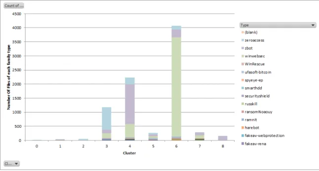
It can be seen that there are three dominant family types in the dataset: Win-websec, Zbot and Zeroaccess. These family types are distinctly seen in three different clusters in the stacked column chart. The family type Winwebsec dominates in Clus-ter 6. The family type Zbot dominates in ClusClus-ter 4. The family type Zeroaccess dominates in Cluster 3. Of all the stacked column charts drawn, though the family types are distinctly seen in the clusters for k = 9. Thus, as per the results, the dataset can be divided into three major clusters, as shown in Figure A.16. From the results in Figure A.16, we obtain the graphs in Figure 8. Clearly, the Winwebsec
Figure 7: Stacked Column Chart for 9 Clusters
Figure 8: Stacked Column Chart for 9 Clusters
family type has malware samples from Cluster 6, the Zbot family type has malware samples from Cluster 4 and the Zeroaccess family type has the malware samples from Cluster 3. The functionality and details of these three clusters corresponding to the malware family types in the decreasing order of their dominance in the dataset can
be explained as follows:
• Cluster 6: Most of the malware samples that fall in the cluster are of type Winwebsec. As described in [46], “Winwebsec is a category of malware that attacks the users of Windows operating system and produce fake claims as gen-uine anti-malware softwares. They show pop-ups that claim to scan for malware and displays fake warnings similar to 32 Virus and Trojans Detected on your computer. Click on Fix Now button to clean these threats. They then show a message to the user that they need to pay money to activate the software in order to remove these threats which actually doesn’t exist. These malware may display a dialog that looks similar to Windows Security Center or it may have names like Live Security Platinum or Security Shield. The GUI varies from variant to variant.” Winwebsec programs generate misleading alerts and false detections in order to convince users to purchase illegitimate security soft-ware [46]. They may also display logos or product names of some well known companies like Microsoft.
• Cluster 4: The second most dominant type in the dataset is Zbot. As described in [28], “Zbot is family of Trojans can steal your personal information and give a hacker access and control of your PC. They can also lower your internet browser security and turn off your firewall. They can be installed on your PC via spam emails and hacked websites, or packaged with other malware families.” It specifically targets system information, online credentials, and banking details, but can be customized through the toolkit to gather any sort of information. This is done by tailoring configuration files that are compiled into the Trojan installer by the attacker [39].
• Cluster 3: The third type which has its dominance in the dataset is Zeroaccess. As per [42], Trojan.Zeroaccess is a Trojan horse that uses an advanced rootkit to hide itself. It can also create a hidden file system, downloads more malware, and opens a back door on the compromised computer. The threat is also capable of downloading other threats on to the compromised computer, some of which may be misleading applications that display bogus information about threats found on the computer and scare the user into purchasing fake antivirus software to remove the bogus threats. It is also capable of downloading updates of itself to improve and/or fix functionality of the threat [42].
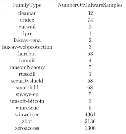
The other family types in the dataset are WinRescue, ufasoft-bitcoin, spyeye-ep, smarthdd, securityshield, russkill, ransom Noaouy, ramnit, harebot, fakeav-webprotection, fakeav-rena. The number of malware samples of these family types is very insignificant. In Table 7, we have tabulated the malware distribution in the dataset for quick reference.
The problem in k-means clustering is that the number of clusters k must be predetermined. We have performed the experiments fork = 2 tok = 15 and identified the best case. The clustering might be more accurate when k is more than 15.
6.2.2 Why is clustering important?
There are many benefits of clustering malware. Firstly, the clustering of malware can allow faster response to new threats – If the new malware can fit in one of the existing clusters, the anti-malware detection and removal are already known. Hence, the new malware can be removed with the known techniques. If it does not fit in one of the clusters, the known techniques of malware detection and removal will not work. Hence, the new techniques need to be found out [2]. Secondly, the clustering of
Table 7: Malware Distribution in the dataset FamilyType NumberOfMalwareSamples cleaman 32 cridex 74 cutwail 2 dprn 1 fakeav-rena 2 fakeav-webprotection 3 harebot 53 ramnit 4 ransomNoaouy 5 russkill 1 securityshield 58 smarthdd 68 spyeye-ep 5 ufasoft-bitcoin 3 winrescue 5 winwebsec 4361 zbot 2136 zeroaccess 1306
malware helps in better understanding of malware activities – The clustering might help us in knowing the functionality of the malware and their relationship with other malware.
CHAPTER 7
Conclusion and Future Work
In this project, we proposed and evaluated the k-means clustering algorithm for classifying over 9000 malware samples. We scored the malware samples using the hidden Markov models for variety of compilers and malware generators (GCC, MINGW, CLANG, TURBOC, TASM and MWOR). We used these scores as the input to thek-means clustering algorithm. Experiments were performed varying the number of clusters from k = 2 to k = 15. We drew the stacked column charts for all the cases. It was observed that the charts for the case k = 9 proved to be the best case. The distinction in the family types of the malware in this case was clearly seen in the clusters. Each cluster corresponds to a specific malware family. The functionality of the three dominating clusters: Winwebsec, Zbot, Zeroaccess was described in Chapter 6. The results showed that HMMs are an effective tool for the challenging task of automatically classifying malware.
In this project, the distances in k-means clustering algorithm are calculated using the Euclidean distance formula. Some other ways of finding the distance – the Hamming distance (also called city block and Manhattan distance), Minkowski distance or cosine distance can be explored in the future work.
The centroid selection of the dataset can be done in a number of ways. In this project, we have computed the cluster centroid by computing the mean for that clus-ter. The k initial means are computed within the data domain. The following varia-tion methods can be tried as a part of the future work: The centroids can be randomly generated within the data domain. k-medians clustering can be explored, wherein the
median in each dimension is calculated instead of the mean [10]. k-medoids cluster-ing can be tried out which calculates the medoid instead of the mean [21]. Fuzzy C-means Clustering, which is a soft version of k-means, where each data point has a fuzzy degree belonging to each cluster [6].
In this project, some of the malware samples are very different than the other malware samples. If we filter out these samples from the dataset, the clustering will be more accurately done. For this, we can calculate the standard deviation of the malware dataset and consider only those samples which fall within certain range (say, 95%) of the standard deviation. The clusters generated in this way must be more meaningful, since the outliers will not be considered.
In this project, we have considered the hidden Markov models for a variety of compilers and malware generators. For the future work, we can consider using only the HMMs for a variety of known malware. Going further, we can train the hidden Markov models for the dominant family types of the malware that exist in the dataset and see how the clusters are formed.
LIST OF REFERENCES
[1] D. Aha, D. Kibler, and M. Albert (1991). Instance-Based Learning Algorithms.
Machine Learning,6, 37–66.
[2] R. Amorim, B. Mirkin, and J. Gan (2012). Anomalous pattern based clustering of mental tasks with subject independent learning. Artificial Intelligence Research, 1(1).
[3] T. Austin, E. Filiol, S. Josse, and M. Stamp (2013). Exploring Hidden Markov Models for Virus Analysis: A Semantic Approach. System Sciences (HICSS), 2013 46th Hawaii International Conference, 5039–5048.
[4] J. Aycock (2006).Computer Viruses and Malware. Fairfax, VA: Springer-Verlag New York.
[5] J. Baltazar, J. Costoya, and R.Flores (n.d.). The Real Face of KOOBFACE: The Largest Web 2.0 Botnet Explained.
http://www.trendmicro.com/cloud-content/us/pdfs/security-intelligence/ white-papers/wp_the-real-face-of-koobface.pdf
[6] J. Bezdek, R. Ehrlich, and W. Full (1984). FCM: The Fuzzy c-Means Clustering Algorithm. Computers & Geosciences, 10(2-3), 191–203.
[7] C. Bishop. (2006).Pattern Recognition and Machine Learning. Springer.
[8] R. Canzanese, M. Kam, and S. Mancoridis (n.d.). Toward an Automatic, Online Behavioral Malware Classifiction System.
https://www.cs.drexel.edu/~spiros/papers/saso2013.pdf
[9] S. Cesare and Y. Xiang (2010). Classification of Malware Using Structured Con-trol Flow. 8th Australasian Symposium on Parallel and Distributed Computing,
107, 61–70.
[10] K. Chen (n.d.). A constant Factor Approximation Algorithm for K-median Clus-tering with Outliers.
http://faculty.cs.tamu.edu/chen/courses/cpsc669/2009/reading/xu1.pdf
[11] F. Cohen (1993). Operating system protection through program evolution. Com-puter & Security, 12(6), 565–584.
[12] C. Cortes and V. Vapnik(1995). Support-Vector Networks. Machine Learning,
[13] S. Deshpande (2012). Eigenvalue Analysis for Metamorphic Detection, Masters Thesis, San Jose State University.
http://scholarworks.sjsu.edu/cgi/viewcontent.cgi?article=1271&context=etd_projects
[14] Difference between a computer virus and a computer worm (n.d.).
http://scienceline.ucsb.edu/getkey.php?key=52
[15] Y. Freund and R. Schapire (1999). A Short Introduction to Boosting. Journal of Japanese Society for Artificial Intelligence, 14(5), 771–780.
[16] F. Howard (2012). Exploring the Blackhole exploit kit: 4.1 Distribution of web threats.
http://nakedsecurity.sophos.com/exploring-the-blackhole-exploit-kit-14/
[17] N. Idika and A. Mathur (2007). A Survey of Malware Detection Techniques.
http://www.flickr.com/photos/panda_security/5198720136/lightbox
[18] Indika (2011). Difference between Hierarchical and Partitional Clustering.
http://www.differencebetween.com/
difference-between-hierarchical-and-vs-partitional-clustering
[19] A. Jain and R. Dubes (1988).Algorithms for Clustering Data. Englewood Cliffs, New Jersey: Prentice Hall.
[20] K. Jones (1972). A statistical interpretation of term specificity and its application in retrieval. Journal of Documentation, 28(1), 11–21.
[21] L. Kaufman and P. Rousseeuw (1987). Clustering by means of Medoids, edited by Y. Dodge.Statistical Data Analysis Based on the L1-Norm and Related Methods,
405–416. North Holland.
[22] S. Kazi and M. Stamp (2013). Hidden Markov Models for software piracy detec-tion. Information Security Journal: A Global Perspective, 22(3), 140–149. [23] S. Kolter and M. Maloof (2006). Learning to Detect and Classify Malicious
Ex-ecutables in the Wild. Journal of Machine Learning Research, 7, 2721–2744. [24] A. Krogh (1998). An Introduction to hidden Markov models for biological
se-quences.Computational Methods in Molecular Biology,45–63. Lyngby, Denmark: Elsevier.
[25] A. Lakhotia, A. Walenstein, C. Miles, and A. Singh (2013). VILO: a rapid learn-ing nearest-neighbor classifier for malware traige.Journal in Computer Virology,
9(3), 109–123. Secaucus, NJ: Springer-Verlag. [26] M. Landesman (n.d.). Boot sector virus repair.
[27] J. MacQueen (1967). Some Methods for Classification and Analysis of Multi-variate Observations. Proceedings of 5-th Berkeley Symposium on Mathematical Statistics and Probability, 1. 281–297. Berkeley, University of California.
[28] Malware Protection Center (n.d.). Win32/Zbot.
http://www.microsoft.com/security/portal/
threat/encyclopedia/entry.aspx?Name=Win32%2fZbot
[29] M. Maron and J. Kuhns (1960). On relevance, probabilistic indexing, and infor-mation retrieval. Journal of the Association for Computing Machinery, 7, 216– 244.
[30] P. Mullins (n.d.). Malware.
http://cs.sru.edu/~mullins/cpsc100book/
module05_SoftwareAndAdmin/module05-04_softwareAndAdmin.html
[31] A. Nappa, M. Zubair Rafique, and J. Caballero (2013). Driving in the Cloud: An Analysis of Drive-by Download Operations and Abuse Reporting of viruses.
Proceedings of the 10th Conference on Detection of Intrusions and Malware & Vulnerability Assessment. Berlin, DE.
[32] Panda Security (n.d.). Virus, worms, trojans and backdoors: Other harmful relatives of viruses.
http://www.pandasecurity.com/homeusers-cms3/security-info/about-malware/generalconcepts/concept-2.htm
[33] Panda Security (n.d.). Malware Evolution.
http://www.flickr.com/photos/panda_security/5198720136/lightbox
[34] S. Priyadarshani (2011). Metamorphic Detection via Emulation, Masters Thesis, San Jose State University.
http://scholarworks.sjsu.edu/cgi/viewcontent.cgi?article=1176&context=etd_projects
[35] L. Rabiner (1989). A tutorial on hidden Markov models and selected applications in speech recognition. Proceedings of the IEEE, 77(2), 257–286.
[36] N. Runwal, R. Low, and M. Stamp (2012). Opcode graph similarity and meta-morphic detection. Journal in Computer Virology, 8, 37–52.
[37] M. Stamp (2011).Information Security: Principles and Practice, second edition, Hoboken, NJ: Wiley-Interscience.
[38] M. Stamp (2012). A Revealing Introduction to Hidden Markov Models.
http://www.cs.sjsu.edu/faculty/stamp/RUA/HMM.pdf
[39] Symantec (2010). Trojan.Zbot.
[40] Symantec (2009). What is the difference between viruses, worms, and Trojans?
http://www.symantec.com/business/support/index?page=content&id=TECH98539
[41] Symantec (2004). Trojan Horse.
http://www.symantec.com/security_response/writeup.jsp?docid=2004-021914-2822-99
[42] Symantec Security Response (2011). Trojan.Zeroaccess.
http://www.symantec.com/security_response/writeup.jsp?docid=2011-071314-0410-99
[43] A. Vasudevan. (2008). MalTRAK: Tracking and Eliminating Unknown Malware.
Computer Security Applications Conference 311-321.
[44] N. Villeneuve with a foreword by R. Deibert &R. Rohozinski (2010). KOOB-FACE: Inside a Crimeware Network.
http://www.trendmicro.com/cloud-content/us/pdfs/
security-intelligence/white-papers/wp_the-real-face-of-koobface.pdf
[45] Virus Bulletin (n.d.). Last-minute paper: An indepth look into Stuxnet.
http://www.virusbtn.com/conference/vb2010/abstracts/LastMinute7.xml
[46] Virus Removal Services (n.d.). Beware of FAKE Antivirus - Winwebsec.
http://virus.myfirstattempt.com/2012/11/beware-of-fake-anti-virus-winwebsec.html
[47] W. Wong and M. Stamp (2006). Hunting for metamorphic engines. Journal in Computer Virology. 2(3), 211–229.
[48] M. Yusoff and A. Jantan (2011). Optimizing Decision Tree in Malware Classifi-cation System by using Genetic Algorithm.
http://sdiwc.net/digital-library/web-admin/upload-pdf/00000060.pdf
[49] Q. Zhang and S. Sun (2012). A centroid k-nearest neighbor method. ADMA’10 Proceedings of the 6th international conference on Advanced data mining and applications: Part I, 278–285. Berlin, Heidelberg: Springer-Verlag.
APPENDIX
Graphs for k-means Clustering Algorithm for Malware Classification
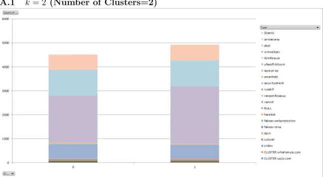
A.1 k = 2 (Number of Clusters=2)
Figure A.9: Stacked Column Chart for 2 Clusters (Uniformly Spaced Initial Cen-troids)
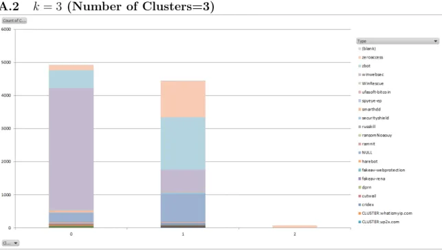
A.2 k = 3 (Number of Clusters=3)
Figure A.10: Stacked Column Chart for 3 Clusters (Uniformly Spaced Initial Cen-troids)
A.3 k = 4 (Number of Clusters=4)
Figure A.11: Stacked Column Chart for 4 Clusters (Uniformly Spaced Initial Cen-troids)
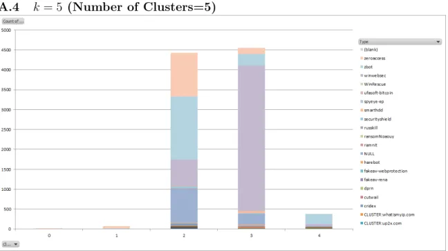
A.4 k = 5 (Number of Clusters=5)
Figure A.12: Stacked Column Chart for 5 Clusters (Uniformly Spaced Initial Cen-troids)
A.5 k = 6 (Number of Clusters=6)
Figure A.13: Stacked Column Chart for 6 Clusters (Uniformly Spaced Initial Cen-troids)
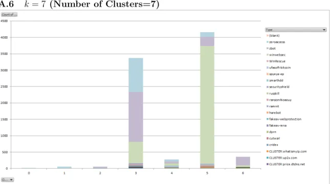
A.6 k = 7 (Number of Clusters=7)
Figure A.14: Stacked Column Chart for 7 Clusters (Uniformly Spaced Initial Cen-troids)
A.7 k = 8 (Number of Clusters=8)
Figure A.15: Stacked Column Chart for 8 Clusters (Uniformly Spaced Initial Cen-troids)
A.8 k = 9 (Number of Clusters=9)
Figure A.16: Stacked Column Chart for 9 Clusters (Uniformly Spaced Initial Cen-troids)
A.9 k = 10 (Number of Clusters=10)
Figure A.17: Stacked Column Chart for 10 Clusters (Uniformly Spaced Initial Cen-troids)
![Figure 1: Malware Growth [33]](https://thumb-us.123doks.com/thumbv2/123dok_us/1077091.2643347/15.918.326.651.601.828/figure-malware-growth.webp)
![Figure 6: A Hidden Markov Model [38]](https://thumb-us.123doks.com/thumbv2/123dok_us/1077091.2643347/22.918.167.736.140.300/figure-a-hidden-markov-model.webp)