Recursive Adaptive Algorithms for Fast and Rapidly
Time-Varying Systems
Yuanjin Zheng, Member, IEEE, and Zhiping Lin, Senior Member, IEEE
Abstract—In this paper, some new schemes are developed to
im-prove the tracking performance for fast and rapidly time-varying systems. A generalized recursive least-squares (RLS) algorithm called the trend RLS (T-RLS) algorithm is derived which takes into account the effect of local and global trend variations of system parameters. A bank of adaptive filters implemented with T-RLS algorithms are then used for tracking an arbitrarily fast varying system without knowing a priori the changing rates of system parameters. The optimal tracking performance is attained by Bayesian a posteriori combination of the multiple filter outputs, and the optimal number of parallel filters needed is determined by extended Akaike’s Information Criterion and Minimum Description Length information criteria. An RLS algorithm with modification of the system estimation covariance matrix is employed to track a time-varying system with rare but abrupt (jump) changes. A new online wavelet detector is designed for accurately identifying the changing locations and the branches of changing parameters. The optimal increments of the covariance matrix at the detected changing locations are also estimated. Thus, for a general time-varying system, the proposed methods can optimally track its slowly, fast and rapidly changing components simultaneously.
Index Terms—Dyadic wavelet transform (DWT), recursive
wavelet change detector, system identification, time-varying system, trend recursive least-squares (T-RLS) algorithm.
I. INTRODUCTION
I
N MANY applications such as speech recognition, commu-nication channel equalization, process control, and biomed-ical signal processing, the underlying time-varying systems are subject to fast and/or rapidly changing environments [1], [4]. To track a fast varying system, several variable-step-size adap-tive algorithms have been proposed to improve the tracking per-formance [1], [3], [4], [8]. However, if the variations of system parameters show obvious deterministic local or global trends, stochastically perturbed difference equation constraints should be used as smooth priors for system parameters [5]. Based on these prior trend models, a multistep algorithm and a KalmanManuscript received March 25, 2002; revised January 22, 2003. This work was supported by the Academic Research Fund, Ministry of Education, Republic of Singapore (RG 42/99). Please note that the review process for this paper was handled exclusively by the TCAS-I editorial office and that the paper has been published in TCAS-II for logistical reasons. This paper was recommended by Associate Editor N. Ling.
Y. Zheng was with the School of Electrical and Electronic Engineering, Nanyang Technological University, Singapore 639798. He is now with the ICS Laboratory, Institute of Microelectronics, Singapore 117685 (e-mail: [email protected]).
Z. Lin is with the School of Electrical and Electronic Engineering, Nanyang Technological University, Singapore 639798 (e-mail: [email protected]).
Digital Object Identifier 10.1109/TCSII.2003.816906
filtering algorithm have been used to track fast varying sys-tems in [6], [7]. Further, when the varying trends of system parameters are unknown, one way to overcome this problem is to assume that the variations of system parameters satisfy a first-order Markov chain model and a multiple adaptive Kalman filtering (MAKF) algorithm is developed for parameter tracking (see, e.g., [9]). Another way is to employ the vector space adap-tive filtering and tracking algorithm [10]. However, the compu-tational loads of all the above methods are heavy and the exact statistical characteristics of system and measurement noises are required.
In this paper, a new trend reciursive least-squares (T-RLS) algorithm is derived for tracking a fast varying system with de-terministic and known trends. One of the advantages of this T-RLS algorithm is that it does not require the exact information on system and measurement noise variances, and state space equation coefficient matrices. Moreover, extended Akaike’s In-formation Criterion (AIC) and Minimum Description Length (MDL) criteria are proposed to determine the optimal order of a time-varying system online. For tracking a general fast varying system with unknown order trends, a multiple T-RLS algorithm is developed which attains the optimal posterior estimation and is computationally simpler than the MAKF algorithm.
When a time-varying system is subject to rare but abrupt (jumping) changes, the estimated parameters by conventional adaptive algorithms cannot track the variations of true system parameters in the vicinity of these jumping locations, resulting in the so called “lag” estimation. Three methods can be used to mitigate the effect of “lag” estimation. The first method is to use variable forgetting factor RLS algorithms [3]. The second is to increase the system estimation covariance matrix at the jumping locations [11], [12]. The third includes various Bayesian Kalman filtering algorithms [13], [14]. In this paper, the second method will be adopted to track the abrupt changes of system parameters. One difficulty of this method is how to identify the unknown locations and amplitudes of the abrupt changes online. Some approaches have been developed toward this task [15]–[18]. The obvious tradeoff between detection sensitivity and robustness exists in these methods. It has been shown that the idea of modification of covariance matrix only with respect to the detected jumping parameter branch(es) would improve the identification accuracy [12], [19]. Hence, it is desirable to have of a simple and yet efficient detection and modification algorithm.
To identify the rapidly changing points effectively, a new on-line detection algorithm based on a multiscale product sequence in wavelet domain is proposed in this paper. The new wavelet detector can efficiently suppress background noise and enhance 1057-7130/03$17.00 © 2003 IEEE
the abruptly changing components so that it is very robust to interferences (with low false alarm probability) and sensitive to jumping changes (with high detection probability) compared with the conventional detectors. A new algorithm for selectively modifying the elements of the covariance matrix is proposed. Moreover, the optimal increments of the covariance matrix are determined.
The rest of the paper is organized as follows. In Section II, a T-RLS algorithm and a multiple T-RLS algorithm are de-veloped which can track an arbitrarily fast varying system. In Section III, a new wavelet detector is proposed for identifying the abrupt changes and a scheme for selectively modifying the estimation covariance matrix is presented for tracking rapidly changing systems. In Section IV, simulation results are provided which verify the superior performance of the proposed algo-rithms. Concluding remarks are given in Section V.
II. RECURSIVEADAPTIVEALGORITHM FORFASTCHANGING SYSTEMS
A. T-RLS Algorithm
A time-varying system commonly can be represented by a linear regression equation and the changes of system parameters can be modeled with an order one (first-order) random walk model [10], [11], [25], [26]
(1) (2) Here, is the true system parameter vector of size , is the scalar observation (output) signal, is the system (input) regressor vector of size , is the system noise vector of
size with covariance matrix , and is the
measurement noise signal with variance . When
the variations of system parameters are slow enough, an RLS algorithm can be used to track the time-varying system [25], [26]
(3) (4) (5)
(6) where is the a priori prediction error, is the filtering gain, is the estimation covariance matrix, and is the forgetting factor.
However, if the time-varying parameters change fast, the first-order random walk model is not sufficient to describe the vari-ations of the system parameters [5], [6]. To accurately model the time-dependent parameters and increase the tracking ability for a fast varying system, a general random walk model can be adopted which sufficiently includes the prior information such as the th order deterministic trend, stochastic trend, and sea-sonal components of a nonstationary process [5]. By this model, Kalman filtering can be employed for system parameter
esti-mation and tracking. However, the explicit statistical charac-teristics of system and measurement noises are required before filtering can be performed [6]. In this subsection, we derive a T-RLS algorithm which can adaptively track fast varying pa-rameters without knowing the explicit statistical characteristics of (possibly nonstationary) system and measurement noises. It is well known that a conventional varying forgetting factor RLS algorithm has to compromise its tracking performance with es-timation variance. Similar to the trend Kalman filter algorithm presented in [5], [6], the proposed T-RLS algorithm can achieve fast tracking and small estimation variance simultaneously.
Assume the system parameters of a fast varying system can be modeled with a general random walk model [7]
(7) (8) where the various prior trend information can be included in a nonsingular matrix with size , and the sizes of and are both of . Obviously, (7) is a more precise model for fast varying system parameters. In the following, assume
that there are available observation samples
and the variables at time represent the initial values in the following. To derive a T-RLS algorithm, rewriting
(7) as and then reversely iterating it
times for , we obtain
(9)
where the inverse transition matrix is defined as if
if (10)
Substituting (9) into (8) for gives
(11)
Define an matrix
(12)
and two vectors
(13)
(14)
Stack (11) in column for and use notations (12)(14) to arrive a vector-matrix equation
From (15), the optimal estimation of system parameters based on observation data (in the sense of weighted least-squares solution) can be obtained as [2]
(16) where denotes a weighting matrix. If takes the inverse of the covariance matrix of the equivalent noise vector , i.e.,
(17) Kalman filtering can be readily derived to achieve an unbiased minimal variance estimation [2]. For deriving the T-RLS algorithm, a reasonable choice is to introduce the following weighting matrix with a set of discounting factors on the diagonal elements [25]:
(18)
where , are discounting factors
defined as
(19) and ( ) is named as the th forgetting factor. Typi-cally, [25], [26]. To derive the recursive estimation equations, define
(20)
Thus
(21) From (21), it is easy to show
(22)
Substituting (12), (13), (19). and (20) into (16) and using (22) gives
(23) The final equality in (23) is just
(24) By applying the matrix inverse lemma [25], (21) can be rewritten in another equivalent form
(25) In summary, for a fast varying system modeled with a gen-eral random walk model (7) and (8), the T-RLS algorithm can be realized by applying (24) and (25) alternatively. Notice that when , (7) and (8) reduce to (1) and (2) and the T-RLS algorithm reduces to the conventional RLS algorithm.
Commonly, we choose with to
simplify the computation. If the order of a general random walk model is properly chosen, commonly takes a value less than but close to 1.
B. Multiple T-RLS Algorithm for Tracking Arbitrarily Fast Varying Systems
If the prior trend information of a fast time-varying system is exactly known, i.e., the matrix is deterministic and known, the T-RLS algorithm can be used for accurate parameter estimation. However, commonly is not explicitly known or even completely unknown. In this case, a bank of T-RLS filters with a spreading of assumed matrices can be performed in parallel for parameter estimation separately and at the same time a Bayesian posterior combination is employed to attain the optimal parameter estimation. We name this scheme as the Multiple T-RLS (MT-RLS) algorithm. The MT-RLS algorithm does not estimate the unknown of a fast varying system directly. Instead, it obtains the optimal parameter estimation
through weighted averaging the multiple adaptive filter outputs. The optimal weighting coefficients can be determined by Bayesian probability inference. It is shown in the following that the MT-RLS algorithm can be realized with quite simple computations and yet has good performance.
For an unknown system (7) and (8) (where matrix , vari-ance of and covariance of all are unknown), T-RLS adaptive filters can be adopted for parallel adaptive filtering. Let the th filter corresponds to the following
hypo-thetical values of the design parameters . The
recursive parameter estimation by the th filter is performed as (26) (27)
(28) where is the assumed trend matrix for the th filter. Without loss of generality, the th priori prediction error is assumed an i.i.d. Gaussian distributed sequence with zero mean and variance [12]. The optimal parameter estimation based on the completed observation sequence
can be obtained as
(29)
where is the posterior probability of the hypothetical model
given the data set , i.e., .
A more general assumption is to consider a nonstationary system where the measurement noise itself possibly changes with time slowly. In this case, since and are both slowly varying, only most recent observation data samples are used to reliably estimate so that is assumed invariant in this
time interval (i.e., ). Denote
, and redefine as
(30) To estimate , Bayes rule can be applied
(31)
The denominator of the above equation is a constant which is not relevant to . Under i.i.d. Gaussian assumption and according to (27), the conditional likelihood function of based on
and is . Thus the
joint conditional likelihood function of recent samples can be represented as
(32)
As in [20], we assign noninformative prior distributions to and as
(33) (34) Substituting (32)–(34) into (31), it is easy to derive
(35)
(36)
Here, and are two different constants. Define
(37)
which can be estimated recursively as
(38)
Since , can be recursively estimated based
on as
(39)
In summary, the MT-RLS algorithm can be recursively imple-mented by (26)–(29), (38), and (39). Like the T-RLS algorithm, the MT-RLS does not require the information of system and measurement noises and, thus, is computationally simpler than the MAKF algorithm. At this point, several parameters ,
and in the MT-RLS algorithm remain to be
selected. In the following section, we will discuss the problem of optimal parameter selection.
C. Parameter Selection for the MT-RLS Algorithm
The filtering length should be chosen to ensure the signal in this interval is approximately stationary, so that can be considered as unchanged and can be estimated efficiently by the observed data set in this interval. Recall that the memory of the
RLS algorithm is approximately if
is less than but close to 1 [25], [26]. Thus, can take
(40)
where means rounding toward positive infinity.
The forms and values of may be chosen by referring to the varying trend of the system parameters to be studied. On the one hand, should be selected general enough to encompass the true type and order of the underlying system. Commonly used trend models include local polynomial trend model, stochastic trend model and local polynomial seasonal component model etc. [5]. On the other hand, taking small number of parallel adap-tive filters can reduce the algorithm complexity and improve the computational efficiency. Therefore, we should find a method to determine the optimal filter number (acting as the bandwidth of the adaptive algorithm), which best balances the algorithm complexity and performance.
For tracking a time-varying system with deterministic but un-known trend, the assumed in (7) can take different (integer) order fixed matrices. For example, if the system parameters are assumed to follow a th order polynomial trend, the th order stochastically perturbed difference equation can be used to rep-resent the dynamics of the system parameters. Hence will be
a fixed matrix with size ( ) as (41), shown at
the bottom of the page, where represents Kronecker product
and . Similarly, if the system parameters
are assumed to follow a th order autoregressive (AR) stochastic trend, is also a fixed matrix but with different elements (see [5] and [6] for details). Taking large orders can improve the tracking ability but also increase the model com-plexity, and taking small orders is computationally simple but will decrease the tracking ability. Obviously, an optimal trend model order can be chosen for an unknown system once the forms and values of are selected. This order can be determined by the AIC or MDL information criteria, etc. [6] which optimally balance model representation ability and model complexity. Assume T-RLS adaptive filters are performed in parallel and the th filter takes trend model order . To determine the optimal trend model order, an extended
AIC or MDL sequence and for the trend model
of the th filter at time can be derived as follows:
(42)
(43) where corresponds to the assumed . For a system with all of the three trends,
(44) where , , and are the model orders of the local poly-nomial trend, the AR trend, and the seasonal trend of the th
filter, respectively. , if and , if
for each . See [5] for more
details. We select the th filter as the most matched filter which
leads to the minimal or , i.e.,
or
(45) and as the optimal integer trend model order. Without loss
of generality, we sort as
(46) To reduce the number of parallel filters while keeping good performance, we can design an MT-RLS algorithm with constant filter number (bandwidth) which can opti-mally balance the algorithm performance and the compu-tational complexity. Explicitly, we take as a constant odd number and the corresponding filter orders as . Here, the filter with tend model order corresponds to the most matched filter, the filter with trend model order corresponds to the least underdetermined filter, the filter with trend model order
.. . .. . .. . (41)
corresponds to the most overdetermined filter in the chosen constant bandwidth ( ) adaptive algorithm.
III. RECURSIVEADAPTIVEALGORITHM FORRAPIDLY CHANGING(JUMPING) SYSTEMS
A. Changing Points Detection for Tracking Rapidly Changing Systems
There are two methods to adjust the RLS algorithm (3)–(6) when it is used for tracking a rapidly changing system. One method is to adaptively adjust the forgetting factor at the rapidly changing points while keeping its nominal values at other locations [3]. The other is to increase the estimation co-variance matrix or at the locations of jumping points so that the filtering gain can be increased significantly to track the rapidly changing components [11]. When using either method, the jumping points need to be known a priori and this com-monly is unrealistic in practice. Therefore, a recursive parameter change detection algorithm is required to identify the locations of jumping points online. Once a jumping change is detected, the above RLS algorithm with changing the forgetting factor or the covariance matrix at the detected jumping point can be adopted.
Some recursive change detection algorithms have been de-veloped in [15]–[18]. An attractive method is the one used by Trigg and Leach (T & L) [15]. In this method, two filtering sig-nals gained from the prediction error signal are used
(47) (48) where denotes absolute value and takes a very small posi-tive value (commonly, ). The T & L detection signal is defined as [15]
(49)
According to the central limiting theorem, is asymptotically Gaussian distributed. It is shown in [15] and [16] that, for small
, is a zero-mean signal with variance approximately as (50)
Assume a detection threshold is . When at time index , a parameter change is considered to have happened [11]. De-notes as the false alarm probability of detection. According
to the Chebyshev’s inequality , the
detection threshold can be chosen as
(51)
From the above, we see that there exists a tradeoff between the false alarm probability and the detection probability of the T & L detector. In the following subsection, we will develop a wavelet domain change detection algorithm which can achieve
much higher detection probability when using the same false alarm probability as the one used by the T & L detector (i.e., using the same detection threshold).
B. Wavelet Jump Detector for Abrupt Change Detection
A dyadic wavelet transform (DWT) of function at time
and scale ( and is the maximum decomposition
scale) can be implemented via a set of discrete digital filters as follows [21], [22] (without loss of generality, the initial
condi-tions are assumed as ):
(52)
where is the equivalent digital
filter of DWT in the th scale. It is odd symmetrical with
re-spect to [i.e., ] and its region of support
(the number of nonzero coefficients) at scale is
[21], [23]. Unfortunately, for each scale is a noncausal filter. Hence, (52) cannot be used for calculating DWT online causally. For detecting the changing points on-line, a recursive DWT algorithm is desired that can calculate the DWT coefficients in different scales once a new observation data sample is available. Assuming the available data sequence
at time is , we consider an extended
se-quence by an even-symmetric
exten-sion of as
. (53)
Denote the DWT of at time and scale as , i.e.,
. We will show in the following theorem that can be online calculated from using an equivalent causal filter. Obviously, if a jumping point of occurring at time can be detected from , it also can be detected from since the even-symmetric extension signal does not alter the jumping point features of the original signal . Since can be recursively calculated online, it should be used instead of
for online detecting the abrupt changes of signal .
Theorem 1:: Let the even-symmetric extension sequence
be given in (53), the DWT of at time and scale can be calculated from as
(54)
where is an equivalent causal filter for
scale defined as
.
(55)
Furthermore, can be recursively calculated as
(56) (57)
Here, , , and are column vectors of size which are defined as follows:
(58) (59) (60) To save space, the proof is omitted here but can be found in [24, pp. 91–92].
We name (54) as a causal DWT of the original signal . The above theorem shows that at time can be recursively cal-culated online using (56) and (57) once a new data sample
ar-rives. The scale filters can be calculated
and stored in advance before performing the recursive causal
DWT. In (52), when . Thus, the filter
coefficients of can be calculated by
ap-plying the iterative DWT algorithm introduced in [21] to a input signal. Once is obtained, can be easily calcu-lated by (55). The filter coefficients of for scale 1–4 can be found in [24].
Now, consider multiscale product of the first scale se-quences in wavelet domain at time index
(61)
Since the wavelet used for DWT in this paper is chosen as the first-order derivative of a smooth function (a cubic spline function, see [21]), the DWT can be interpreted as the derivative of local smooth (average) of at scale [22]. Hence, if (thus ) has some singular points (especially jumping points), will appear as modulus maxima at these locations. More importantly, the amplitude of noise modulus maxima will decrease from small scales to large scales while the amplitude of signal modulus maxima will increase from small scales to large scales in the wavelet domain [21], [22]. Therefore, multiscale product sequence sharpens and enhances the modulus maxima dominated by signal edges and at the same time suppresses the modulus maxima dominated by noises. It has been further shown in that the probability density function (PDF) of a multiscale product sequence is heavy tailed compared with that of a Gaussian distributed one with the same variance. Employing these characteristics, a DWT multiscale product sequence of an existing detection signal (for example, obtained from the T & L detector) can be used as a new detection signal. It will enhance the components representing possible abrupt changes in the original detection signal and thus a larger detection threshold can be used, which will lead to a smaller false alarm probability. At the same time, it will suppress the noise interference components in the original detection signal, which will decrease the miss alarm probability and thus increase the detection probability. Motivated by the above discussion, a new wavelet jump detector is now proposed for online change detection.
Denote as the causal DWT of the T & L detection signal (49) at time and scale . That is
(62) which can be recursively calculated as (56) and (57). The mul-tiscale product signal of the first scales can be calculated as
(63)
Define a new (multiscale product) detection signal by filtering as follows:
(64) where is an exponential smoothing factor which commonly takes a value in the range [0.05, 0.13]. Although is heavy-tailed non-Gaussian distributed, obtained above is a Gaussian distributed signal according to the central limiting theorem. Now, a new wavelet detector can be formed as
(65)
Obviously, if is a Gaussian distributed signal, is also a Gaussian distributed signal whose variance is the same as that of . However, if has some local maxima (minima) corre-sponding to the abrupt changes of the original signal, these local maxima (minima) will be enlarged and sharpened in . This characteristics can be employed to provide a more robust and accurate identification of the possible abrupt changes. Thus, if we choose the detection threshold of the wavelet detection signal equal to the threshold of the T & L detection signal , we can achieve much higher detection probability. To get the accurate estimation of the variance of ( ) in (65), a robust method will be proposed shortly based on an empirical equation. We first postulate two transformations as follows.
First, the log of the ratio of the variance of to the variance of satisfies an order polynomial function of
(66)
where . Taking log operation can compress the dynamic
range of and hence an order polynomial
function is sufficient to approximate the log function in the left side of (66).
Second, the log of the ratio of the variance of to the
vari-ance of satisfies a log function plus a linear
function of
(67)
If is a white-noise sequence, the variance
ratio is and thus
[obtained by taking variance on both sides of (64)]. Although wavelet transform
can decorrelate a signal to some degree, in (62) is a correlated signal since is highly correlated. Therefore, in (63) is a correlated signal. A linear function of is added in (67) to account for the bias produced by the correlation of signal .
Combining (66) and (67), the ratio of the variance of new wavelet multiscale product detection signal to the variance of the T & L detection signal (R–W–TL) is defined as
(68) and the wavelet detector (65) using the empirical variance ratio estimation (68) can be represented as
(69)
where the values of , , and can be
esti-mated by applying least-squares method to experimental data through Monte Carlo simulations. Recommendation
values are , , , and
. Extensive simulations have verified that the empirical equations (68) and (69) are effective and produce quite accurate results (see [11] for more details).
C. Selectively Tracking of Rapidly Changing Systems Using Wavelet Jump Detectors
For a time-varying system, different branches of system parameters are not always subject to abrupt changes simul-taneously when a jump occurs. When modifying the matrix
or [in (5) or (6)] with , it is common to select as a diagonal matrix where each diagonal element reflects the change of the corresponding parameter branch. When one or several branches have changed rapidly at a specific time , the corresponding elements in should be increased while the remaining elements should keep unchanged [11]. This requires that the jump detector cannot only identify the locations where the jumps have happened but also determine the branches pro-ducing these jumps.
It is well known that the priori prediction error signal can be used to construct the jump detector [15], [16]. However, this detector (named as prediction detector) only can determine where a jump happens for a time-varying system. To judge which branches this jump is produced by, a set of jump detec-tors can be constructed directly from the estimated filtering gains (named as gain detectors). Combining the prediction
detector with gain detectors, a new selective wavelet detector
is proposed in the following, which can determine not only the locations of jumping points but also the branches that have produced the jumps.
Assume a wavelet detector (prediction detector) is obtained from the priori prediction error signal [see
(4)]. Assume other wavelet detectors (gain
detectors) are obtained from the estimated filtering gains
[see (5)], respectively. Without loss of generality, we assume here a system jumping change at a specific time is produced by an abrupt change of only one parameter branch (the case of several parameter branches changing at the same time is a simple extension). The proposed
selective wavelet detector uses both the prediction detector
and the gain detectors for parameter change detection. More explicitly, an abrupt change is considered to be detected at the
th parameter branch at time , if
and (70)
where the detection threshold is set as and, thus, can be determined by (51) in advance. At this time , we set
. To determine the value of , consider the following equality (see [25, Appendix 3.D]):
(71) (72) where is the sum of the a priori prediction mean-square er-rors at time . When is close to 1, we can take
and is the measurement noise variance [25]. Modify the
matrix as (setting )
(73) Substituting (73) into (71) gives
(74)
Thus, can be estimated as
(75) Similarly, modify the matrix as (setting )
(76) Substituting (76) into (72), and can be estimated as
(77) In a summary, we list the complete RLS algorithm using es-timation covariance matrix modification and selective wavelet detector (abbreviated as RLS-MSWD) at time as follows.
• (a) RLS algorithm
Using (3)–(6) to calculate , , and ; • (b) Selective wavelet detector for change detection
— (b1) From , calculating (47)–(49), (62) [imple-mented with (56) and (57)], (63), (64), (68), and (69) to get the predictive detector ,
— (b2) For : {Using instead of in (47)
and (48), calculating equations as in (b1) to get the th
gain detector } End
— (b3) Using (70) to detect if a jumping change has hap-pened. If yes, determine which parameter branch
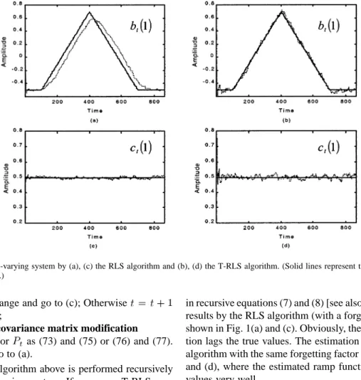
pro-Fig. 1. Track a ramp time-varying system by (a), (c) the RLS algorithm and (b), (d) the T-RLS algorithm. (Solid lines represent true values and dotted lines represent estimation results.)
duces this change and go to (c); Otherwise and go to (a);
• (c) Estimation covariance matrix modification Modify or as (73) and (75) or (76) and (77).
and go to (a).
The RLS-MSWD algorithm above is performed recursively to track a rapidly changing system. If we use a T-RLS or a MT-RLS algorithm instead of the RLS algorithm in step (a) and keep steps (b) and (c) unchanged, the extended algorithm can identify and track an arbitrary time-varying system with slowly, fast and rapidly varying components simultaneously. A typical example will be used in the next section to illustrate this promising tracking method.
IV. SIMULATIONRESULTS
The T-RLS and RLS algorithm are used for tracking a ramp function in Fig. 1. The system simulated is an
model
where is a ramp-like function, is a constant and is assumed a random pulse input. The measurement noise variance of takes 0.01. The RLS algorithm is used for the identification of the above system assuming that the system parameters are modeled with an order one random walk model. The T-RLS algorithm is used for the identification of the same system assuming that the system parameters are modeled with a second order deterministic trend model, where
we take vector , vector
, and matrix
in recursive equations (7) and (8) [see also (41)]. The estimation results by the RLS algorithm (with a forgetting factor 0.97) are shown in Fig. 1(a) and (c). Obviously, the estimated ramp func-tion lags the true values. The estimafunc-tion results by the T-RLS algorithm with the same forgetting factor are shown in Fig. 1(b) and (d), where the estimated ramp function can track the true values very well.
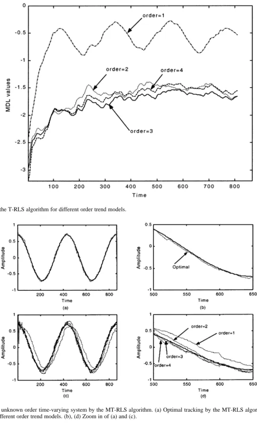
In Figs. 2 and 3, we show that the performance of a MT-RLS
algorithm. An system with as sin-like function
and as a constant is simulated. Here we assume that the true order of the trend model used for modeling system parameters is unknown. The MDL values for assumed deterministic trend model order from 1 to 4 are calculated and shown in Fig. 2. The forgetting factor is taken as 0.98 and thus . We can see that the third-order trend model is the best matched model since its MDL sequence values are minimal among the four MDL sequences of different order trend models after the algorithm converges. If we select the number of parallel filters , the three filters should take the trend models with orders 2, 3, and 4 respectively. The optimal posterior estimation by the MT-RLS algorithm using these three filters is shown in Fig. 3(a), and the estimation results by the T-RLS algorithm using order 1–4 trend model are shown in Fig. 3(c) respectively. Fig. 3(b) and (d) are the zoom-in parts of Fig. 3(a) and (c), respectively. Obviously, the adaptive filter taking order 1 or 2 trend model underestimates the true system parameters while the adaptive filter taking order 3 or 4 trend model overestimates the true system parameters. Thus, we can infer that the true trend model order is between 2–3 but closer to 3. Although we cannot estimate the true trend model order accurately, the optimal estimation of system parameters can still be obtained by the MT-RLS algorithm.
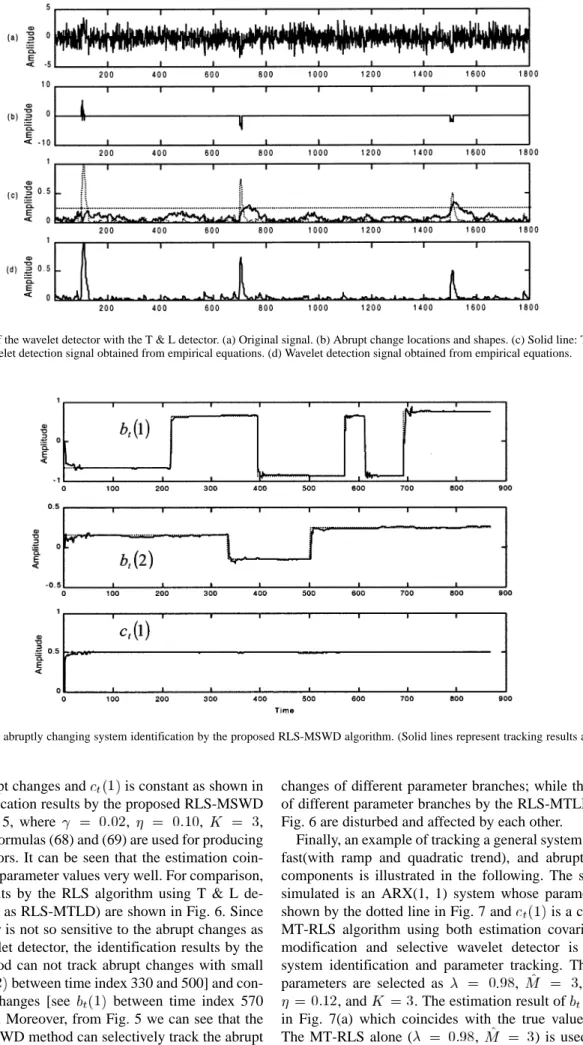
In Fig. 4, the proposed wavelet detector is compared with the T & L detector. Fig. 4(a) shows a stationary white Gaussian noisy signal which has three abrupt changes at the vicinity of
Fig. 2. MDL values of the T-RLS algorithm for different order trend models.
Fig. 3. Track a sin-like unknown order time-varying system by the MT-RLS algorithm. (a) Optimal tracking by the MT-RLS algorithm. (c) Tracking by the T-RLS algorithm with different order trend models. (b), (d) Zoom in of (a) and (c).
time locations 100, 700, and 1500, respectively. The amplitudes and shapes of these changes are shown in Fig. 4(b). In Fig. 4(c), the solid line represents the T & L detection signal and the dotted line represents the wavelet detection signal obtained using the theoretical R–W–TL. Fig. 4(d) shows the same trace as the one represented by the dotted line in Fig. 4(c), i.e., wavelet detection signal obtained using the theoretical R–W–TL (wavelet decomposition scale number ). Comparing the wavelet detection signal with the T & L detection signal in
Fig. 4(c), the former can provide sharper and more accurate indication of the abrupt changing points and this is very important for detecting small amplitude or/and concentrated abrupt changes.
Next, an ARX(2, 1) system
is used to verify the performance of the proposed abrupt change tracking algorithm. Here, the system parameters and
Fig. 4. Comparison of the wavelet detector with the T & L detector. (a) Original signal. (b) Abrupt change locations and shapes. (c) Solid line: T & L detection signal; dotted line: wavelet detection signal obtained from empirical equations. (d) Wavelet detection signal obtained from empirical equations.
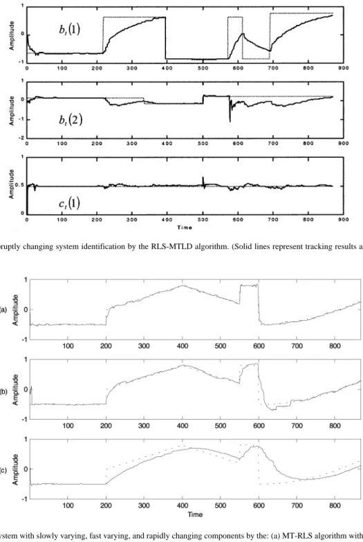
Fig. 5. An ARX(2, 1) abruptly changing system identification by the proposed RLS-MSWD algorithm. (Solid lines represent tracking results and dotted lines represent true values.)
are both with abrupt changes and is constant as shown in Fig. 5. The identification results by the proposed RLS-MSWD
are shown in Fig. 5, where , , ,
and the empirical formulas (68) and (69) are used for producing the wavelet detectors. It can be seen that the estimation coin-cides with the true parameter values very well. For comparison, identification results by the RLS algorithm using T & L de-tector (abbreviated as RLS-MTLD) are shown in Fig. 6. Since the T & L detector is not so sensitive to the abrupt changes as the selective wavelet detector, the identification results by the RLS-MTLD method can not track abrupt changes with small amplitude [see between time index 330 and 500] and con-centrated abrupt changes [see between time index 570 and 620] in Fig. 6. Moreover, from Fig. 5 we can see that the proposed RLS-MSWD method can selectively track the abrupt
changes of different parameter branches; while the estimation of different parameter branches by the RLS-MTLD method in Fig. 6 are disturbed and affected by each other.
Finally, an example of tracking a general system with slowly, fast(with ramp and quadratic trend), and abruptly changing components is illustrated in the following. The system to be simulated is an ARX(1, 1) system whose parameter is shown by the dotted line in Fig. 7 and is a constant. The MT-RLS algorithm using both estimation covariance matrix modification and selective wavelet detector is applied for system identification and parameter tracking. The algorithm
parameters are selected as , , ,
, and . The estimation result of is shown in Fig. 7(a) which coincides with the true values very well.
Fig. 6. An ARX(2, 1) abruptly changing system identification by the RLS-MTLD algorithm. (Solid lines represent tracking results and dotted lines represent true values.)
Fig. 7. Track a general system with slowly varying, fast varying, and rapidly changing components by the: (a) MT-RLS algorithm with covariance modification using selective wavelet detector; (b) MT-RLS algorithm; (c) RLS algorithm. (Solid lines represent tracking results and dotted lines represent true values.) parameter estimation and the result is shown in Fig. 7(b).
Although the trend changes of time-varying parameters are estimated well, this method cannot track the abrupt changes sufficiently. The estimation by the RLS method ( ) is shown in Fig. 7(c) which fails to track both the fast and the abruptly changing components.
V. CONCLUSION
In this paper, the problem of tracking fast and abruptly changing systems has been tackled. A T-RLS algorithm has been proposed to track fast changing parameters with local and global trends. For an unknown fast varying system, a MT-RLS
algorithm has been developed to optimally estimate the system parameters through Bayesian posterior combination of multiple adaptive filter outputs. To track an abruptly changing system, a new online wavelet detector has been proposed which is computationally simpler and can achieve much higher detection probability than commonly used abrupt detection methods. Selectively tracking the rapidly changing parameter branches via estimation covariance modification at the jumping points has been rigorously discussed. Both the jumping locations and increment values of covariance matrix for the detected pa-rameter branches can be determined. Combining the proposed MT-RLS algorithm with the covariance modification method using wavelet detectors, slowly, fast, and abruptly changing
components of a general time-varying system all can be tracked well.
REFERENCES
[1] P. E. Wellstead and M. B. Zarrop, Self-Tuning Systems: Control and
Signal Processing. New York: Wiley, 1991.
[2] C. K. Chui and G. Chen, Kalman Filtering With Real-Time
Applica-tions. Berlin, Germany: Springer-Verlag, 1999.
[3] T. R. Fortescue, L. S. Kershenbaum, and B. E. Ydstie, “Implementation of self-tuning regulators with variable forgetting factor,” Automatica, vol. 17, no. 6, pp. 831–835, 1981.
[4] D. G. Childers, J. C. Principle, and Y. T. Ting, “Adaptive WRLS-VFF for speech analysis,” IEEE Trans. Speech Audio Processing, vol. 3, pp. 209–213, May 1995.
[5] G. Kitagawa and W. Gersch, “A smoothness priors-state space modeling of time-series with trend and seasonality,” J. Amer. Stat. Assoc., vol. 79, pp. 378–389, 1984.
[6] , “A smoothness priors time-varying AR coefficient modeling of nonstationary covariance time-series,” IEEE Trans. Automat. Contr., vol. AC-30, no. 1, pp. 48–56, 1985.
[7] A. Benvensite, “Design of adaptive algorithms for the tracking of time-varying systems,” Int. J. Adapt. Control Signal Process., vol. 1, pp. 3–29, 1987.
[8] S. Haykin, Adaptive Filter Theory, 4th ed. Upper Saddle River, NJ: Prentice-Hall, 2002.
[9] E. Emre and J. Seo, “A unifying approach to multitarget tracking,” IEEE
Trans. Aerosp. Electron. Syst., vol. 25, pp. 520–528, July 1989.
[10] G. A. Williamson, “Tracking random walk systems with vector space adaptive filters,” IEEE Trans. Circuits Syst. II, vol. 42, pp. 543–547, Aug. 1995.
[11] L. Ljung and S. Gunnarsson, “Adaptation and tracking in system iden-tification—A survey,” Automatica, vol. 26, no. 1, pp. 7–21, 1990. [12] M. J. Chen and J. P. Norton, “Estimation technique for tracking rapid
parameter changes,” Int. J. Control, vol. 45, no. 4, pp. 1387–1398, 1987. [13] P. Andersson, “Adaptive forgetting in recursive identification through multiple models,” Int. J. Control, vol. 42, no. 5, pp. 1175–1193, 1985. [14] M. Niedzwiecki, “Identification of time-varying systems with abrupt
pa-rameter changes,” Automatica, vol. 30, no. 3, pp. 447–459, 1994. [15] D. W. Trigg and A. G. Leach, “Exponential smoothing with an adaptive
response rate,” Oper. Res., vol. 18, pp. 53–59, 1967.
[16] B. Carlsson, “Digital differentiating filters and model based fault detec-tion,” Ph.D. dissertation, Dept. Automat. Control, Uppsala Univ., Upp-sala, Sweden, 1989.
[17] T. Hägglund, “New estimation techniques for adaptive control,” Ph.D. dissertation, Dept. Automat. Control, Lund Inst. Technol., Lund, Sweden, 1983.
[18] M. Basseville and I. V. Nikiforov, Detection of Abrupt Changes: Theory
and Application. Englewood Cliffs, NJ: Prentice-Hall, 1993. [19] J. Holst and N. K. Poulsen, “Self tuning control of plant with abrupt
changes,” in Proc. IFAC 9th Triennial World Congr., Budapest, Hungary, 1984, pp. 923–928.
[20] M. Niedzwiecki, “Identification of Nonstationary Stochastic systems using parallel estimation schemes,” IEEE Trans. Automat. Contr., vol. 35, pp. 329–334, Mar. 1990.
[21] S. Mallat and S. Zhong, “Characterization of signals from multiscale edges,” IEEE Trans. Pattern Anal. Machine Intell., vol. 14, pp. 710–732, July 1992.
[22] S. Mallat and W. L. Hwang, “Singularity detection and processing with wavelets,” IEEE Trans. Inform. Theory, vol. 38, pp. 617–643, Feb. 1992. [23] B. M. Sadler and A. Swami, “Analysis of multiscale products for step detection and estimation,” IEEE Trans. Inform. Theory, vol. 45, pp. 1043–1051, Mar. 1999.
[24] Y. J. Zheng, “Contributions to nonstationary adaptive signal processing and time-varying system identification,” Ph.D. dissertation, School Elect. Electron. Eng., Nanyang Technol. Univ., Singapore, 2002. [25] L. Ljung and T. Soderstrom, Theory and Practice of Recursive
Identifi-cation. Cambridge, MA: MIT Press, 1983.
[26] L. Ljung, System Identification: Theory for the User. Upper Saddle River, NJ: Prentice-Hall, 1997.
Yuanjin Zheng (M’03) received the B.Eng. degree with first class honors and the M.Eng. degree with best graduate student honors from Xi’an Jiaotong Uni-versity, Xi’an, China, in 1993 and 1996, respectively, and the Ph.D. degree from Nanyang Technological University, Singapore, in 2001.
From July 1996 to April 1998, he was with the National Key Lab of Optical Communication Technology, University of Electronic Science and Technology of China, as a Research Assistant. In March 2001, he joined the Institute of Mi-croelectronics, Singapore, as a Senior Research Engineer. His research is cur-rently focused on communication system design and performance evaluation, analog and digital IC design, and DSP algorithm design and implementation. He has authored over 15 papers published in international journals and confer-ence proceedings. He is the holder of four U.S. patents pending.
Zhiping Lin (M’86–SM’00) received the Ph.D. degree in information engi-neering from the University of Cambridge, Cambridge, U.K., in 1987.
He was with the University of Calgary, Calgary, AB, Canada, from 1987 to 1988, with Shantou University, China, from 1988 to 1993, and with DSO National Laboratories, Singapore, from 1993 to 1999. Since 1999, he has been an Associate Professor in the School of Electrical and Electronic Engineering, Nanyang Technological University, Singapore. His research interests include multidimensional systems and signal processing, wavelets, and biomedical signal processing.
Dr. Lin is currently on the Editorial Board of Multidimensional Systems and
Signal Processing and is an Associate Editor of Circuits, Systems, and Signal Processing.