ACCURATE SUM AND DOT PRODUCT∗
TAKESHI OGITA †, SIEGFRIED M. RUMP ‡, AND SHIN’ICHI OISHI §
Abstract. Algorithms for summation and dot product of floating point numbers are presented which are fast in terms of measured computing time. We show that the computed results are as accurate as if computed in twice orK-fold working precision,K≥3. For twice the working precision our algorithms for summation and dot product are some 40 % faster than the corresponding XBLAS routines while sharing similar error estimates. Our algorithms are widely applicable because they require only addition, subtraction and multiplication of floating point numbers in the same working precision as the given data. Higher precision is unnecessary, algorithms are straight loops without branch, and no access to mantissa or exponent is necessary.
Key words. accurate summation, accurate dot product, fast algorithms, verified error bounds, high precision
AMS subject classifications. 15-04, 65G99, 65-04
1. Introduction. We present fast algorithms to compute approximations of high quality of the sum and the dot product of floating point numbers. We show that results share the same error estimates as if computed in twice or K-fold working precision and rounded back to working precision (for precise meaning, see Subsection 1.2).
We interpret fast not only in terms of floating point operations (flops) but in terms of measured computing time. Our algorithms do not require other than one working precision. Since summation and dot product are most basic tasks in numerical analysis, there are numerous algorithms for that, among them [6, 9, 11, 14, 17, 18, 19, 20, 22, 25, 26, 27, 28, 29, 31, 34, 35, 36, 37, 38, 41]. Higham [15] devotes an entire chapter to summation. Accurate summation or dot product algorithms have various applications in many different areas of numerical analysis. Excellent overviews can be found in [15, 26].
1.1. Previous work. We collect some notes on previous work to put our results into suitable perspective; our remarks are by no means complete. Dot products can be transformed into sums, therefore much effort is concentrated on accurate summation of floating point numbers. In the following we assume the computer arithmetic to satisfy the IEEE 754 standard [2].
Many approaches to diminish rounding errors in floating point summation sort input data by absolute value. If all summands are of the same sign, increasing ordering is best. However, if summation is subject to cancellation, decreasing order may be superior [15]. A major drawback of such approaches is that optimization of code by today’s compilers is substantially jeopardized by branches.
Floating point summation is frequently improved by compensated summation. Here, a cleverly designed correction term is used to improve the result. One of the first is the following one due to Dekker [10].
∗This research was partially supported by 21st Century COE Program (Productive ICT Academia
Program, Waseda University) from the Ministry of Education, Science, Sports and Culture of Japan.
†Graduate School of Science and Engineering, Waseda University, 3-4-1 Okubo Shinjuku-ku,
Tokyo 169-8555, Japan ([email protected]).
‡Institut f¨ur Informatik III, Technische Universit¨at Hamburg-Harburg, Schwarzenbergstraße 95,
Hamburg 21071, Germany ([email protected]).
§Department of Computer Science, School of Science and Engineering, Waseda University, 3-4-1
Okubo Shinjuku-ku, Tokyo 169-8555, Japan ([email protected]). 1
Algorithm 1.1. Compensated summation of two floating point numbers.
function [x, y] =FastTwoSum(a, b) x= fl(a+b)
y= fl((a−x) +b)
For floating point arithmetic with rounding to nearest and base 2, e.g. IEEE 754 arithmetic, Dekker [10] showed in 1971 that the correction is exact if the input is ordered by magnitude, that is
x+y=a+b (1.1)
provided |a| ≥ |b|. A similar correction is used in the Kahan-Babuˇska algorithm [3, 32, 31], and in a number of variants (e.g. [16, 31]). Those algorithms are almost ideally backward stable, that is for floating point numberspi,1≤i≤n, the computed
sum ˜ssatisfies ˜ s= n X i=1 pi(1 +εi), |εi| ≤2eps+O(eps2). (1.2)
An interesting variant of the Kahan-Babuˇska algorithm was given by Neumaier [31]. The result ˜sof Algorithm IV in his paper satisfies
|s˜− n X i=1 pi| ≤eps| n X i=1 pi|+ (0.75n2+n)eps2 n X i=1 |pi|, for 3neps≤1. (1.3)
Without knowing, Neumaier uses Dekker’s Algorithm 1.1 ensuring|a| ≥ |b| by com-parison. Neumaier’s result is of a qualityas if computed in twice the working precision and then rounded into working precision. If input data is sorted decreasingly by ab-solute value, Priest showed that two extra applications of the compensation process produces aforward stable result of almost optimal relative accuracy [37].
However, branches may increase computing time due to lack of compiler optimiza-tion. Already in 1969, Knuth [23] presented a simple algorithm (that is Algorithm 3.1 (TwoSum) in this paper) to computexandy satisfying (1.1) regardless of the magni-tude ofa and b. The algorithm requires 6 flops without branch. Counting absolute value and comparison as one flop, Dekker’s Algorithm 1.1 with ensuring |a| ≥ |b|
by comparison requires 6 flops as well; however, because of less optimized code, it is up to 50 % slower than Knuth’s method. Therefore we will develop branch-free algorithms to be fast in terms of execution time. Combining Kahan-Babuˇska’s and Knuth’s algorithm is our first summation algorithmSum2.
Knuth’s algorithm, like Dekker’s with sorting, transforms any pair of floating point numbers (a, b) into a new pair (x, y) with
x= fl(a+b) and a+b=x+y.
We call an algorithm with this property error-free transformation. Such trans-formations are in the center of interest of our paper. Extending the principle of an error-free transformation of two summands to nsummands is called “distillation algorithms” by Kahan [21]. Here input floating point numberspi,1≤i≤n, are
trans-formed into p(ik) with Pni=1pi =
Pn
i=1p (k)
use sorting of input data by absolute value leading to a computing timeO(nlogn) for addingnnumbers. An interesting new distillation algorithm is presented by Anderson [1]. He uses a clever way of sorting and deflating positive and negative summands. However, branches slow down computations, see Section 6.
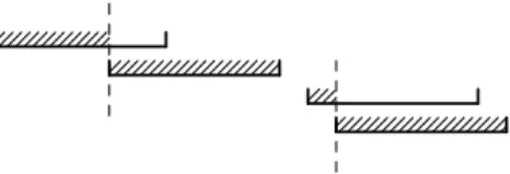
Another transformation is presented by Priest [36]. He transforms input numbers pi,1≤i≤ninto a non-overlapping sequenceqi, such that the mantissa bit of lowest
significance of qi is greater than the one of highest significance of qi+1 (see Figure
1.1).
Fig. 1.1.Non-overlapping sequence by Priest’s scheme
Shewchuk [41] weakens this into nonzero-overlapping sequences as shown in Figure 1.2. This means that mantissa bits of qi and qi+1 may overlap, but only if the
corresponding bits of qi are zero. He shows that this simplifies normalization and
improves performance.
Fig. 1.2. Nonzero-overlapping sequence by Shewchuk’s scheme
Quite different approaches use the fact that due to the limited exponent range, all IEEE 754 double precision floating point numbers can be added in a superlong accu-mulator (cf. Kulisch and Miranker [24]). Doubling the size of the accuaccu-mulator creates algorithms for dot products as well. Splitting mantissas and adjustment according to exponents requires some bit manipulations. The result within the long accumulator represents theexact sum or dot product and can be rounded to the desired precision. A simple heuristic to improve the accuracy of matrix products is implemented in INTLAB [39]. Matrices of floating point numbers A = (aij), B = (bij) are first
split into A =A1+A0 and B =B1+B0, where the (i, j)-th entries of A1 andB1
comprise of the first M significant bits of aij and bij, respectively. For IEEE 754
double precision we chooseM = 17. The matrix productA·B is then approximated byA1·B1+ (A1·B0+A0·B). The heuristic is that for not too large dimension and
for inputaij, bij not differing too much in magnitude, the productA1·B1is exact, so
that the final approximation is of improved accuracy. This method is implemented in the routinelssresidual for residual correction of linear systems in INTLAB.
Another interesting and similar approach was recently presented by Zielke and Drygalla [44]. They split input numberspi according to the scheme in Figure 1.3.
The chunks of maximallyM bits start at the most significant bit of all input data pi. For proper choice of M depending onn and the input format, summation of the
most significant chunks is exact. Cancellation can be monitored by the magnitude of the previous sum when adding the next chunks. Note that in the INTLAB method
Mbits Mbits Mbits
Fig. 1.3.Zielke and Drygalla’s scheme
the splitting for all matrix entries is independent of the exponent of the entries and can be performed without branch, whereas here the splitting is individual for every matrix element. On the other hand, the method by Zielke and Drygalla allows to compute a forward stable result of the dot product. The advantage over the long accumulator approach is that the amount of work is determined by the condition of the problem.
Recently, Demmel and Hida presented algorithms using a wider accumulator [11]. Floating point numbers pi,1 ≤ i ≤ n, given in working precision with t bits in
the mantissa are added in an extra-precise accumulator with T bits, T > t. Four algorithms are presented with and without sorting input data. The authors give a detailed analysis of the accuracy of the result depending ont,T and the number of summands. In contrast to our methods which use only working precision they need in any case some extra-precise floating point format.
Finally, XBLAS [26], the Extended and Mixed Precision BLAS, contains algo-rithms based on [4, 5] which are very similar to ours. However, XBLAS treats lower order terms of summation and dot product in a more complicated way than ours resulting in an increase of flop count of about 40 %. In the same computing time as XBLAS our algorithms can produce an accurate result for much more ill-conditioned dot products. For details, see Sections 4 and 5, and for timing and accuracy see Section 6.
With respect to theresult of a summation or dot product algorithm we can grossly distinguish three different approaches:
i) heuristic/numerical evidence for improvement of result accuracy, ii) result accuracy as if computed in higher precision,
iii) result with prescribed accuracy.
Algorithms of the second class are backward stable in the sense of (1.2) with respect to a certaineps, whereas algorithms of the third class are forward stable in a similar sense. Our methods belong to the second class and, with small modifications described below, to the third class. To our knowledge all known methods belonging to the second or third class except the new XBLAS approach [26] bear one or more of the following disadvantages:
• sorting of input data is necessary, either i) by absolute value or,
ii) by exponent,
• the inner loop contains branches,
• besides working precision, some extra (higher) precision is necessary,
• access to mantissa and/or exponent is necessary.
Each of those properties may slow down the performance significantly and/or restrict application to specific computers or compilers. In contrast, our approach uses only floating point addition, subtraction and multiplication in working precision
without any of those disadvantages.
1.2. Our goal. We will present algorithms for summation and dot product with-out branch using only one working precision to compute a resultsof the same quality
as if computed in K-fold precision and rounded to working precision. This means the following.
Let floating point numbers pi,1 ≤i≤n, witht-bit precision be given. We call
that working precision. Then the resultsshall satisfy
|s− n X i=1 pi| ≤eps|s|+ (ϕeps)K n X i=1 |pi|, (1.4)
with a moderate constantϕandeps:= 2−t. The second term in the right hand side
of (1.4) reflects computationK-fold precision, and the first one rounding back into working precision.
1.3. Our approach. Our methods are based on iterative application of error-free transformations. This has been done before, Shewchuk for example uses such a scheme for sorted input data to produce nonzero-overlapping sequences [41].
We extend the error-free transformation of two floating point numbers to vectors of arbitrary length (Algorithm 4.3, VecSum) and use it to compute a result as if
computed in twice the working precision. Then we show that iterative (K-1)-fold application of VecSum can be used to produce a result as if computed in K-fold working precision (Algorithm 4.8,SumK).
Furthermore, Dekker and Veltkamp [10] gave an error-free transformation of the product into the sum of two floating point numbers. We use this to create dot product algorithms with similar properties as our summation algorithms.
Moreover, we give simple criteria to check theaccuracyof the result. This check is also performed in working precision and in rounding to nearest. Nevertheless it allows to compute valid error bounds for the result of a summation and of a dot product.
The structure of our algorithms is clear and simple. Moreover, the error-free trans-formations allow elegant error estimations diminishing involved battles with rounding error terms to a minimum. All error analysis is due to the second author.
1.4. Outline of the paper. The paper is organized as follows. After introduc-ing notation we briefly summarize the algorithms for error-free summation and dot product of two floating point numbers and their properties. In Section 4 we present and analyze our algorithms for summation corresponding to 2-fold (i.e. doubled) and to K-fold working precision, and in the next section we do the same for the dot product. In Section 6 numerical examples for extremely ill-conditioned problems are presented, as well as timing, accuracy, comparison with other algorithms and some remarks on practical applications. In the concluding remarks we address possible implications for the design of the hardware of digital computers.
2. Notation. Throughout the paper we assume a floating point arithmetic ad-hering to IEEE 754 floating point standard [2]. We assume that no overflow occurs, but allow underflow. We will use only one working precision for floating point com-putations. If this working precision is IEEE 754 double precision, this corresponds to 53 bits precision including an implicit bit. The set of working precision floating point numbers is denoted byF, the relative rounding error unit byeps, and the underflow unit byeta. For IEEE 754 double precision we haveeps= 2−53 andeta= 2−1074.
We stress that IEEE 754 arithmetic is not necessary if the error-free transforma-tionsTwoSumandTwoProductto be described in the next section are available.
We denote by fl(·) the result of a floating point computation, where all operations inside the parentheses are executed in working precision. If the order of execution is ambiguous and is crucial, we make it unique by using parentheses. Floating point operations according to IEEE 754 satisfy [15]
fl(a◦b) = (a◦b)(1 +ε1)
= (a◦b)/(1 +ε2) for◦ ∈ {+,−}and|εν| ≤eps,
and
fl(a◦b) = (a◦b)(1 +ε1) +η1
= (a◦b)/(1 +ε2) +η2 for◦ ∈ {·, /}and|εν| ≤eps,|ην| ≤eta.
Addition and subtraction is exact in case of underflow [13], andε1η1 =ε2η2= 0 for
multiplication and division. This implies
|a◦b−fl(a◦b)| ≤ eps|a◦b|
|a◦b−fl(a◦b)| ≤ eps|fl(a◦b)| for◦ ∈ {+,−},
(2.1) and
|a◦b−fl(a◦b)| ≤ eps|a◦b|+eta
|a◦b−fl(a◦b)| ≤ eps|fl(a◦b)|+eta for◦ ∈ {·, /}
(2.2)
for all floating point numbersa, b∈F, the latter becauseε1η1=ε2η2= 0. Note that
a◦b∈Rand fl(a◦b)∈F, but in generala◦b /∈F. It is known [29, 10, 7, 8] that the approximation error of floating point operations is itself a floating point number:
x= fl(a±b) ⇒ a±b=x+y for y∈F, x= fl(a·b) ⇒ a·b=x+y for y∈F, (2.3)
where no underflow is assumed for multiplication. Similar facts hold for division and square root but are not needed in this paper. These are error-free transformations of the pair (a, b) into (x, y), where xis the result of the corresponding floating point operation. Note that no information is lost; the equalities in (2.3) are mathematical identities for all floating point numbersa, b∈F.
Throughout the paper the number of flops of an algorithm denotes the num-ber of floating point operations counting additions, subtractions, multiplications and absolute value separately.
We use standard notation and standard results for our error estimations. The quantitiesγn are defined as usual [15] by
γn:= neps
1−neps forn∈N.
When using γn, we implicitly assume neps < 1. For example, for floating point
numbersai∈F, 1≤i≤n, this implies [15, Lemma 8.4]
a= fl à n X i=1 ai ! ⇒ |a− n X i=1 ai| ≤γn−1 n X i=1 |ai|. (2.4)
Note that this result holds independent of the order of the floating point summation and also in the presence of underflow. We mention that we are sometimes a little generous with our estimates, for example, replacing γ4n−2 byγ4n, or an assumption
3. Error-free transformations. Our goal is to extend the error-free transfor-mations for the sum and product of two floating point numbers to vector sums and to dot products. Therefore, (2.3) will play a fundamental role in the following. For-tunately, the quantities x, y are effectively computable, without branches and only using ordinary floating point addition, subtraction and multiplication. For addition we will use the following algorithm by Knuth [23].
Algorithm 3.1. Error-free transformation of the sum of two floating point numbers.
function [x, y] =TwoSum(a, b) x= fl(a+b)
z= fl(x−a)
y= fl((a−(x−z)) + (b−z))
We use Matlab-like [43] notation. Algorithm 3.1 transforms two input floating point numbersa, binto two output floating point numbersx, y such that [23]
a+b=x+y and x= fl(a+b). (3.1)
The proof for that [23] is also valid in the presence of underflow since addition and subtraction is exact in this case.
The multiplication routine needs to split the input arguments into two parts. For the numbertgiven byeps= 2−t, we defines:=dt/2e; in IEEE 754 double precision
we havet= 53 ands= 27. The following algorithm by Dekker [10] splits a floating point numbera∈Finto two partsx, y, where both parts have at mosts−1 nonzero bits. In a practical implementation, “factor” can be replaced by a constant.
Algorithm 3.2. Error-free splitting of a floating point number into two parts.
function [x, y] =Split(a)
c= fl(factor·a) % factor= 2s+ 1
x= fl(c−(c−a)) y= fl(a−x)
It seems absurd that a 53-bit number can be split into two 26-bit numbers. However, the trick is that Dekker uses one sign bit in the splitting. Note also that no access to mantissa or exponent of the input “a” is necessary, standard floating point operations suffice.
The multiplication to calculate “c” in Algorithm 3.2 cannot cause underflow ex-cept when the input “a” is deep in the gradual underflow range. Since addition and subtraction is exact in case of underflow, the analysis [10] ofSplit is still valid and we obtain
a=x+y and xandy nonoverlapping with|y| ≤ |x|.
With this the following multiplication routine by G.W. Veltkamp (see [10]) can be formulated.
Algorithm 3.3. Error-free transformation of the product of two floating point numbers. function [x, y] =TwoProduct(a, b) x= fl(a·b) [a1, a2] =Split(a) [b1, b2] =Split(b) y= fl(a2·b2−(((x−a1·b1)−a2·b1)−a1·b2))
Note again that no branches, only basic and well optimizable sequences of floating point operations are necessary. In case no underflow occurs, we know [10] that
a·b=x+y and x= fl(a·b).
In case of underflow of any of the five multiplications in Algorithm 3.3, suppose the algorithm is performed in a floating point arithmetic with the same length of mantissa but an exponent range so large that no underflow occurs. Denote the results by x0
andy0. Then a rudimentary analysis yields|y0−y| ≤5eta. We do not aim to improve
on that because underflow is rare and the quantities are almost always negligible. We can summarize the properties of the algorithmsTwoSum and TwoProduct as follows.
Theorem 3.4. Let a, b∈F and denote the results of Algorithm 3.1(TwoSum)by
x, y. Then, also in the presence of underflow,
a+b=x+y, x= fl(a+b), |y| ≤eps|x|, |y| ≤eps|a+b|. (3.2)
The algorithm TwoSumrequires 6 flops.
Let a, b∈Fand denote the results of Algorithm 3.3(TwoProduct)byx, y. Then, if no underflow occurs,
a·b=x+y, x= fl(a·b), |y| ≤eps|x|, |y| ≤eps|a·b|, (3.3)
and in the presence of underflow,
a·b=x+y+ 5η, x= fl(a·b), |y| ≤eps|x|+ 5eta, |y| ≤eps|a·b|+ 5eta (3.4)
with|η| ≤eta. The algorithmTwoProduct requires 17 flops.
Proof. The assertions follow by (2.1), (2.2), [23], [10] and the fact that addition and subtraction is exact in the presence of underflow.
Note that the approximation errory=a·b−xis frequently available inside the processor, but inaccessible to the user. If this information were directly available, the computing time of TwoProduct would reduce to 1 flop. Alternatively, TwoProduct can be rewritten in a simple way if a Fused-Multiply-and-Add operation is available as in the Intel Itanium and many other processors (cf. [33]). This means that for a, b, c∈Fthe result ofFMA(a, b, c) is the rounded-to-nearest exact resulta·b+c∈R. Then Algorithm 3.3 can be replaced by
Algorithm 3.5. Error-free transformation of a product using Fused-Multiply-and-Add.
function [x, y] =TwoProductFMA(a, b) x= fl(a·b)
y=FMA(a, b,−x)
This reduces the computing time for the error-free transformation of the product to 2 flops. As FMAis a basic task and useful in many algorithms, we think a round-to-nearest sum ofthree floating point numbers is such. SupposeADD3(a, b, c) is a floating point number nearest to the exact suma+b+c∈Rfora, b, c∈F. Then Algorithm 3.1 can be replaced by
Algorithm 3.6. Error-free transformation of addition usingADD3.
function [x, y] =TwoSumADD3(a, b) x= fl(a+b)
y=ADD3(a, b,−x)
This reduces the error-free transformation of the addition also to 2 flops. We will comment on this again in the last section.
4. Summation. Let floating point numbers pi ∈ F, 1 ≤ i ≤ n, be given. In
this section we aim to compute a good approximation of the sum s =Ppi. With
Algorithm 3.1 (TwoSum) we have a possibility to addtwofloating point numbers with
exact error term. So we may try to cascade Algorithm 3.1 and sum up the errors to improve the result of the ordinary floating point summation fl (Ppi).
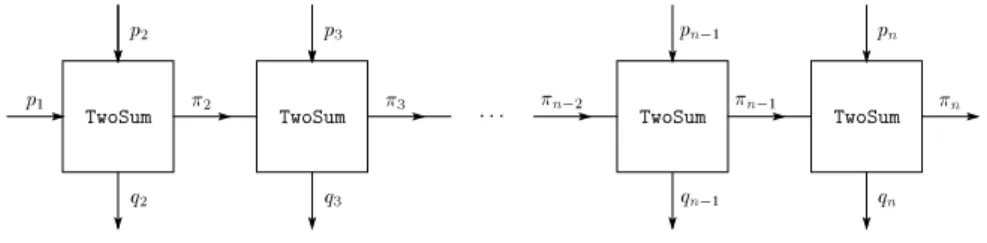
TwoSum TwoSum TwoSum TwoSum
p 1 p 2 p 3 p n 1 p n 2 3 n 2 n 1 n q2 q3 q n 1 qn
Fig. 4.1.Cascaded error-free transformation
Each of the boxes in Figure 4.1 represents Algorithm 3.1 (TwoSum), the error-free summation of two floating point numbers. A cascaded algorithm summing up error terms is as follows.
Algorithm 4.1. Cascaded summation.
functionres=Sum2s(p) π1=p1; σ1= 0;
fori= 2 :n
[πi, qi] =TwoSum(πi−1, pi)
σi = fl(σi−1+qi)
res= fl(πn+σn)
Algorithm 4.1 is a compensated summation [15]. The well known Kahan-Babuˇska al-gorithm [32] is Alal-gorithm 4.1 usingFastTwoSuminstead ofTwoSum. Since the transfor-mation [πi, qi] =FastTwoSum(πi−1, pi) is only proved to be error-free if|πi−1| ≥ |pi|,
the result of the Kahan-Babuˇska algorithm is in general of less quality than Algorithm 4.1. Neumaier’s Algorithm IV in [31] improves Kahan-Babuˇska by ordering |πi−1|,
|pi|before applyingFastTwoSum . So it is mathematically identical to Algorithm 4.1
and only slowed down by sorting. For the error analysis we first note
πn= fl à n X i=1 pi ! and σn= fl à n X i=2 qi ! (4.1)
which follows by successive application of (3.2). Soπnis the result of ordinary floating
terms. The error-free transformation by each application of TwoSum allows an exact relation between the inputpi, the errorsqi and the floating point resultπn. We have
πn=πn−1+pn−qn=πn−2+pn−1−qn−1+pn−qn=π1+ n X i=2 (pi−qi), so that s= n X i=1 pi=πn+ n X i=2 qi. (4.2)
In other words, without the presence of rounding errors the result “res” of Algorithm 4.1 would be equal to the exact sums=Ppi. We also note the well known fact that
adding up the errors needs not necessarily improve the final result. Consider p= [1 θ θ2 −θ −θ2 −1]
(4.3)
with a floating point numberθ∈Fchosen small enough that fl(1 +θ) = fl(1−θ) = 1 and fl(θ+θ2) = fl(θ−θ2) = θ. Then Table 4.1 shows the intermediate results of
Algorithm 4.1.
Table 4.1
Intermediate results of Algorithm 4.1 for (4.3)
i pi πi qi σi 1 1 1 0 2 θ 1 θ θ 3 θ2 1 θ2 θ 4 −θ 1 −θ 0 5 −θ2 1 −θ2 −θ2 6 −1 0 0 −θ2
The table implies
res= fl(π6+σ6) =−θ2 whereasπ6= fl
³X pi
´
= 0 =Xpi=s.
So ordinary summation accidentally produces the exact result zero, whereas Algorithm 4.1 yieldsres=−θ2. In other words, we cannot necessarily expect improvement of
the accuracy of the result by using Algorithm 4.1 instead of ordinary summation. However, we can show that the error bound improves significantly. Our algorithms produce, as we will see, a resultas if computed in higherprecision. For the proof of the first corresponding theorem on that we need a technical lemma.
Lemma 4.2. Let floating point numbers β0 ∈F andbi∈F,1≤i≤n, be given. Suppose the floating point numbersci, βi∈F,1≤i≤n, are computed by the following loop. fori= 1 :n [βi, ci] =TwoSum(βi−1, bi) Then n X i=1 |ci| ≤γn−1 n X i=1 |bi| forβ0= 0, (4.4)
and n X i=1 |ci| ≤γn à |β0|+ n X i=1 |bi| ! for general β0∈F. (4.5)
Proof. The second inequality (4.5) is an immediate consequence of the first one (4.4), so we assumeβ0= 0. For later use we state
γn−1+eps(1 +γn)≤ (n−1)eps
1−neps + eps
1−neps =γn. (4.6)
We proceed by induction and note that for n = 1 we have β1 = b1 and c1 = 0.
Suppose (4.4) is true for somen≥1. Then βn+1= fl Ãn+1 X i=1 bi ! , and (3.2) and (2.4) imply
|cn+1| ≤eps|βn+1| ≤eps(1 +γn) n+1
X
i=1
|bi|.
Using the induction hypothesis and (4.6) yields
nX+1 i=1 |ci| ≤γn−1 n X i=1 |bi|+eps(1 +γn) n+1 X i=1 |bi| ≤γn n+1 X i=1 |bi|.
Before analyzing Algorithm 4.1 (TwoSum), we stress that it can be viewed as an
error-free vector transformation: The n-vector p is transformed into the n-vector [q2...nπn] with properties similar to (3.1):
i) Pn i=1 pi= n P i=2 qi+πn=s ii) πn= fl µ n P i=1 pi ¶ . (4.7)
To underline this, we rewrite the first part of Algorithm 4.1 so that the vector entries are overwritten. This results in the following compact notation.
Algorithm 4.3. Error-free vector transformation for summation.
functionp=VecSum(p) fori= 2 :n
[pi, pi−1] =TwoSum(pi, pi−1)
The vectorpis transformed without changing the sum, andpnis replaced by fl (
P pi).
Kahan [21] calls this a “distillation algorithm”. The following algorithm is equivalent to Algorithm 4.1, the results “res” are identical.
Algorithm 4.4. Cascaded summation equivalent to Algorithm 4.1.
functionres=Sum2(p) fori= 2 :n [pi, pi−1] =TwoSum(pi, pi−1) res= fl µµn−1 P i=1 pi ¶ +pn ¶
Proposition 4.5. Suppose Algorithm 4.4 (Sum2) is applied to floating point numberspi∈F,1≤i≤n, sets:=
P
pi∈RandS:=
P
|pi|and supposeneps<1. Then, also in the presence of underflow,
|res−s| ≤eps|s|+γn2−1S.
(4.8)
Algorithm 4.4 requires 7(n−1) flops. If Algorithm 3.6(TwoSumADD3) is used instead of Algorithm 3.1(TwoSum), then Algorithm 4.4 requires3(n−1)flops.
Remark 1. The final result “res” is calculated as a floating point sum in the last line of Algorithm 4.4 or, equivalently, in Algorithm 4.1. The exact result “s” is, in general, not a floating point number. Therefore we cannot expect an error bound (4.8) better than eps|s|. Besides that, the error bound (4.8) tells that the quality of the result “res” is as if computed in doubled working precision and rounded to working precision.
Remark 2. The important point in the analysis is the estimation of the er-ror of the final summation fl(πn +σn). A straightforward analysis includes a term
eps|πn|, for which the only bound we know is epsS. This, of course, would ruin the
whole analysis. Instead, we can use the mathematical property (4.2) of the error-free transformationTwoSumimplying thatπn+
P
qi−sis equal to zero.
Remark 3. It is very instructive to express and interpret (4.8) in terms of the condition number of summation. The latter is defined forPpi6= 0 by
cond³Xpi ´ := lim ε→0sup ½¯ ¯ ¯ ¯ P e pi− P pi εPpi ¯ ¯ ¯ ¯: |pe| ≤ε|p| ¾ ,
where absolute value and comparison is to be understood componentwise. Obviously cond³Xpi ´ = P |pi| |Ppi| = S |s|. (4.9)
Inserting this into (4.8) yields
|res−s| |s| ≤eps+γ 2 n−1·cond ³X pi ´ .
In other words, the bound for the relative error of the result “res” is essentially (neps)2 times the condition number plus the inevitable summandeps for rounding
the result to working precision.
Remark 4. Neumaier’s [31] proves for his mathematically identical Algorithm IV the similar estimation
|res−s| ≤eps|s|+ (0.75n2+n)eps2S ,
provided 3neps≤1. His proof is involved.
Proof of Proposition 4.5. For the analysis of Algorithm 4.4 we use the equivalent formulation Algorithm 4.1. In the notation of Algorithm 4.1 we know by (4.4)
n X i=2 |qi| ≤γn−1 n X i=1 |pi|=γn−1S. (4.10)
Thenσn= fl ( Pn i=2qi) and (2.4) imply |σn− n X i=2 qi| ≤γn−2 n X i=2 |qi| ≤γn−2γn−1S. (4.11)
Furthermore,res= fl(πn+σn) meansres= (1 +ε)(πn+σn) with |ε| ≤eps, so that
in view of (4.2), |res−s| = |fl(πn+σn)−s|=|(1 +ε)(πn+σn−s) +εs| = |(1 +ε)(πn+ n P 2 qi−s) + (1 +ε)(σn− n P i=2 qi) +εs| ≤ (1 +eps)|σn− n P i=2 qi|+eps|s| ≤ (1 +eps)γn−2γn−1S+eps|s|, (4.12)
and the result follows by (1 +eps)γn−2≤γn−1.
The high precision summation in XBLAS [26] is fairly similar to Algorithm 4.4 except that lower order terms are treated a different way. The corresponding algorithm BLAS_dsum_xin [26] is as follows:
Algorithm 4.6. XBLAS quadruple precision summation.
functions=SumXBLAS(p) s= 0; t= 0; fori= 1 :n [t1, t2] =TwoSum(s, pi) t2=t2+t; [s, t] =FastTwoSum(t1, t2)
Lower order terms are added inSumXBLASusing an extra addition and Algorithm 1.1 (FastTwoSum) to generate a pair [s, t] with s+t approximating Ppi in quadruple
precision. Omitting the last statement in Algorithm 4.1 (or equivalently in Algorithm 4.4, Sum2) it follows by (4.7, i)) and (4.11) that the pair [πn, σn] is of quadruple
precision as well. Output of SumXBLAS is the higher order part s which satisfies a similar error estimate as Sum2. However, XBLAS summation requires 10n flops as compared to 7(n−1) flops forSum2. For timing and accuracy see Section 6.
The error bound (4.8) for the resultresof Algorithm 4.4 is not computable since it involves the exact valuesof the sum. Next we show how to compute a valid error bound in pure floating point in round to nearest, which is also less pessimistic. We use again the notation of the equivalent Algorithm 4.1. Following (4.12) and (4.11) we have
|res−s| = |fl(πn+σn)−s| ≤eps|res|+|σn+πn−s|
≤ eps|res|+|Pn i=2 qi+πn−s|+γn−2 n P i=1 |qi|
≤ eps|res|+ (1 +eps)n−2γ n−2fl( n P i=1 |qi|) ≤ eps|res|+γ2n−4α , where α := fl(Pn i=2
|qi|). If meps < 1 for m ∈ N, then fl(meps) = meps ∈ F and
computation ofγm=meps/(1−meps). Therefore
γm≤(1−eps)−1fl(meps/(1−meps)).
The floating point multiplication fl(eps|res|) may cause underflow, so setting β := fl(2neps/(1−2neps)α) and being a little generous with the lower order terms shows
|res−s| ≤ fl(eps|res|) + (1−eps)4γ
2nα+eta
≤ (1−eps)fl(eps|res|) + (1−eps)3fl(2neps/(1−2neps))α
+eps·fl(eps|res|) +eta
≤ (1−eps)fl(eps|res|) + (1−eps)2β+ fl(eps2|res|) + 2eta
≤ (1−eps)fl(eps|res|) + (1−eps)2β
+ (1−eps)3fl(2eps2|res|) + (1−eps)33eta
≤ (1−eps)fl(eps|res|) + (1−eps)2β
+ (1−eps)2fl¡2eps2|res|+ 3eta¢
≤ (1−eps)fl(eps|res|) + (1−eps)fl¡β+ (2eps2|res|+ 3eta)¢
≤ fl¡eps|res|+¡β+ (2eps2|res|+ 3eta)¢¢ .
The following corollary translates the result into the notation of Algorithm 4.4.
Corollary 4.7. Let floating point numberspi∈F,1≤i≤n, be given. Append the statements
if 2neps≥1,error(’dimension too large’),end β= (2neps/(1−2neps))· µn−1 P i=1 |pi| ¶
err=eps|res|+ (β+ (2eps2|res|+ 3eta) )
(to be executed in working precision) to Algorithm 4.4(Sum2). If the error message is not triggered,errsatisfies
res−err≤Xpi≤res+err.
This is also true in the presence of underflow. The computation oferrrequires2n+ 8
flops.
For later use we estimate the sum of the absolute values of the transformed vector. Using (4.2) and (4.10) we obtain
n X i=2 |qi|+|πn|= n X i=2 |qi|+|s− n X i=2 qi| ≤ |s|+ 2 n X i=2 |qi| ≤ |s|+ 2γn−1S. (4.13)
Denoting the output vector of Algorithm 4.3 (VecSum) byp0 this means n X i=1 |p0i| ≤ ¯ ¯ ¯ ¯ ¯ n X i=1 pi ¯ ¯ ¯ ¯ ¯+ 2γn−1 n X i=1 |pi|. (4.14)
If summation of thepi is not too ill-conditioned (up to condition numbereps−1,
say), the result of Algorithm 4.4 (Sum2) is almost maximally accurate and there is nothing more to do. Suppose the summation is extremely ill-conditioned with con-dition number beyond eps−1. Then the vector pis transformed bySum2 into a new
vector p0 with p0
n being the result of ordinary floating point summation in working
precision. Because of ill-condition, p0
n is subject to heavy cancellation, so |p0n| is of
the orderepsP|pi|. Moreover, (4.14) implies that
P
|p0
By (4.9) this means thatSum2 transforms a vector pi being ill-conditioned with
respect to summation into a new vector with identical sum but condition number improved by about a factor eps. This is the motivation to cascade the error-free vector transformation. Our algorithm is as follows.
Algorithm 4.8. Summation as in K-fold precision by (K−1)-fold error-free vector transformation.
functionres=SumK(p, K) fork= 1 :K−1 p=VecSum(p) res= fl µµn−1 P i=1 pi ¶ +pn ¶
Note that forK = 2, Algorithm 4.8 (SumK) and Algorithm 4.4 (Sum2) are identical. To analyze the behavior of Algorithm 4.8 denote the input vector pbyp(0), and the
vectorpafter finishing loopk byp(k).
Lemma 4.9. With the above notations setS(k):=Pn i=1|p
(k)
i |for0≤k≤K−1. Then the intermediate results of Algorithm 4.8(SumK)satisfy the following:
i) s:= Pn i=1 p(0)i =Pn i=1 p(ik) for1≤k≤K−1, ii) |res−s| ≤eps|s|+γ2 n−1S(K−2), iii) S(k)≤3|s|+γk
2n−2S(0) provided4(n−1)eps≤1and1≤k≤K−1.
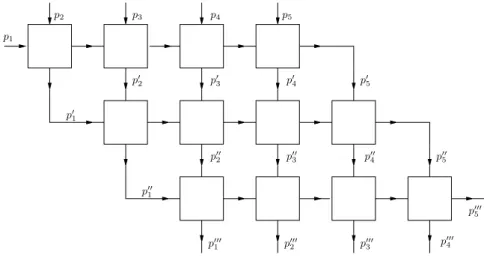
Remark. Before we prove this result, consider the scheme in Figure 4.2 explain-ing the behavior of Algorithm 4.8 forn= 5 andK= 4. For simplicity we replacep(0)i bypi, and denote p(ik) bypi withk-fold prime.
p1 p′1 p′′1 p′′′5 p3 p2 p4 p5 p′2 p′3 p′4 p′5 p′′2 p′′3 p′′4 p′′5 p′′′1 p′′′2 p′′′3 p ′′′ 4 1
Fig. 4.2. Outline of Algorithm 4.8 forn= 5andK= 4
Proof of Lemma 4.9. Figure 4.2 illustrates the (K−1)-fold application of the main loop of Algorithm 4.3 or, equivalently, the first three lines of Algorithm 4.1. Therefore, i) follows by successive application of (4.2). Usings =Pni=1p(iK−2) and
applying Proposition 4.5 yieldsii). To proveiii), successive application of (4.14) and usingi) gives S(2)≤ |s|+ 2γ n−1(|s|+ 2γn−1S(0)) and S(k)≤ |s| ∞ X i=0 (2γn−1)i+ (2γn−1)kS(0) for 1≤k≤K−1. We have ∞ X i=0 (2γn−1)i= 1 1− 2(n−1)eps 1−(n−1)eps = 1−(n−1)eps 1−3(n−1)eps . If 4(n−1)eps≤1, then 1−(n−1)eps≤3(1−3(n−1)eps) and
1−(n−1)eps 1−3(n−1)eps ≤3, so
S(k)≤3|s|+ (2γ
n−1)kS(0) .
Using 2γm≤γ2m yieldsiii).
Insertingiii) of Lemma 4.9 into ii) proves the following error estimate for Algo-rithm 4.8.
Proposition 4.10. Let floating point numbers pi ∈ F, 1 ≤ i ≤ n, be given and assume 4neps≤1. Then, also in the presence of underflow, the result “res” of Algorithm 4.8(SumK)satisfies forK≥3
|res−s| ≤(eps+ 3γ2
n−1)|s|+γK2n−2S, where s :=Ppi and S :=
P
|pi|. Algorithm 4.8 requires (6K−5)(n−1) flops. If Algorithm 3.6(TwoSumADD3)is used instead of Algorithm 3.1(TwoSum), then Algorithm 4.8 requires(2K−1)(n−1)flops.
We mention that the factors γν in Proposition 4.10 are conservative (see the
computational results in Section 6). Moreover, the term 3γ2
n−1is negligible compared
toeps. So the result tells that with each new loop onkthe error estimate drops by a factor of sizeeps, and the final result is of quality as if computed inK-fold precision. The extra term eps|s| reflects the rounding into working precision. This is the best we can expect.
Corollary 4.11. Assume4neps<1. The result “res” of Algorithm 4.8(SumK), also in the presence of underflow, satisfies
|res−s| |s| ≤eps+ 3γ 2 n−1+γ2Kn−2·cond ³X pi ´ .
In other words, the bound for the relative error of the result “res” is essentially the relative rounding error unit eps plus(ϕeps)K times the condition number for a moderate factorϕ.
Note that Corollary 4.11 illustrates the unusual phenomenon that for very ill-conditioned input the computed result is more accurate than cond ×eps. This is solely due to the fact that all intermediate transformationsTwoSuminSumKare error-free – although individual operations withinTwoSumare afflicted with rounding errors. The usual heuristic applies only to the last line of Algorithm 4.8 (SumK).
We mention that Algorithm 4.8 can be used to achieve a certainaccuracy using the rigorous error estimate in Corollary 4.7 to determine a suitable value ofK.
Algorithm 4.8 (SumK) proceeds through the scheme in Figure 4.2 horizontally. This bears the advantage that one may continue if the desired accuracy is not yet achieved. However, a local vector of lengthnis necessary if the input vector shall not be overwritten. To overcome this problem, we may as well proceedvertically through the scheme in Figure 4.2. In this case the number of lines, i.e.K−1, has to be specified in advance. Note thatK is usually very small, so the number of intermediate results is negligible, only some K values. The final result is exactly the same because all transformations are error-free!
Algorithm 4.12. Equivalent formulation of Algorithm 4.8 – vertical mode.
functionres=SumKvert(p, K) K= min(K, n) fori= 1 :K−1 s=pi fork= 1 :i−1 [qk, s] =TwoSum(qk, s) end qi=s end fori=K:n α=pi fork= 1 :K−1 [qk, α] =TwoSum(qk, α) end s=s+α end forj= 1 :K−2 α=qj fork=j+ 1 :K−1 [qk, α] =TwoSum(qk, α) end s=s+α end res=s+qK−1
The algorithm divides into three parts, the initialization (leading upper triangle), the main part of the loop and the final lower triangle in Figure 4.2.
5. Dot product. With Algorithm 3.3 (or Algorithm 3.5) we already have an error-free transformation of the product of two floating point numbers into the sum of two floating point numbers. Combining this with our summation algorithms yields a first algorithm for the computation of the dot product of twon-vectorsx, y.
Algorithm 5.1. A first dot product algorithm.
fori= 1 :n
[ri, rn+i] =TwoProduct(xi, yi)
res=SumK(r, K)
For the moment we assume that no underflow occurs. Then, P2i=1n ri =xTy. With
these preliminaries and noting that the vectorrhas 2nelements we can easily analyze Algorithm 5.1.
Theorem 5.2. Let xi, yi ∈ F, 1 ≤i ≤n, be given and denote by res∈ F the result of Algorithm 5.1. Assume4neps<1. Then forK≥2and without the presence of underflow,
|res−xTy| ≤(eps+ 3γ22n−1)|xTy|+γ4Kn|xT| |y|.
Algorithm 5.1 requires6K(2n−1) + 7n+ 5or less than(12K+ 7)nflops. ForK= 2
these are31n−7flops. IfTwoSumADD3andTwoProductFMAis used instead ofTwoSum
andTwoProduct, respectively, then Algorithm 5.1 requires2K(2n−1) + 1flops, which are8n−3 flops forK= 2.
Proof. In view of Proposition 4.10, (3.3) and P2i=1n ri = xTy we only need to
estimateS:=P2i=1n |ri|. By (3.3), 2n X i=1 |ri| ≤ n X i=1 |fl(xiyi)|+eps n X i=1 |xiyi| ≤(1 + 2eps)|xT| |y|,
so that Proposition 4.10 yields
|res−xTy|=¯¯res− 2n X i=1 ri ¯ ¯ ≤(eps+ 3γ2 2n−1)|xTy|+γ4Kn−2(1 + 2eps)|xT| |y| ≤(eps+ 3γ2 2n−1)|xTy|+γ4Kn|xT| |y|.
In the following we will improve Algorithm 5.1 first for K = 2, and then for generalK≥3.
The most frequently used application of an improved dot product is the compu-tation in doubled working precision, corresponding toK= 2 in Algorithm 5.1. In this case the remainders rn+i are small compared tori, and we can improve the
perfor-mance by adding those remainders in working precision instead of usingTwoSum. This reduces the number of flops from 31nto 25n. Furthermore we will obtain an improved error estimate in Proposition 5.5 and especially Corollary 5.7, most beautiful and the best we can expect. Our algorithm forK= 2 corresponding to a result as if computed in twice the working precision is as follows.
Algorithm 5.3. Dot product in twice the working precision.
functionres=Dot2(x, y) [p, s] =TwoProduct(x1, y1) fori= 2 :n [h, r] =TwoProduct(xi, yi) [p, q] =TwoSum(p, h) s= fl(s+ (q+r)) res= fl(p+s)
An inspection yields
p= fl(xTy),
so that the final result “res” of Algorithm 5.3 is the ordinary floating point resultpof the dot product plus the summed up error termss. If there is not much cancellation in xTy, then the approximation pis dominant, whereas the error term stakes over
for an ill-conditioned dot product. For the analysis we rewrite Algorithm 5.3 into the following equivalent one.
Algorithm 5.4. Equivalent formulation of Algorithm 5.3.
functionres=Dot2s(x, y)
[p1, s1] =TwoProduct(x1, y1) fori= 2 :n [hi, ri] =TwoProduct(xi, yi) [pi, qi] =TwoSum(pi−1, hi) si= fl(si−1+ (qi+ri)) res= fl(pn+sn)
For the analysis of Algorithm 5.4 (and therefore of Algorithm 5.3), for the moment still assuming no underflow occurred, we collect some facts about the intermediate results. By (3.3) we have fori≥2,
qi+ri = (pi−1+hi−pi) + (xiyi−hi) =xiyi+pi−1−pi, and therefore s1+ n X i=2 (qi+ri) = (x1y1−p1) + Ã n X i=2 xiyi+p1−pn ! =xTy−p n. (5.1)
Applying (3.3), Lemma 4.2 and again (3.3) yields
|s1| ≤ eps|x1y1|, n P i=2 |qi| ≤ γn−1(|p1|+ n P i=2 |hi|) =γn−1 n P i=1 |fl(xiyi)| ≤(1 +eps)γn−1|xT| |y|, n P i=2 |ri| ≤ eps n P i=2 |xiyi|, and with
eps+ (1 +eps)γn−1=eps+(1 +eps)(n−1)eps
1−(n−1)eps = neps 1−(n−1)eps we obtain |s1|+ n P i=2 |qi|+ n P i=2 |ri| ≤ eps|xT| |y|+ (1 +eps)γn−1|xT| |y| = neps 1−(n−1)eps|x T| |y|. (5.2)
For later use we apply (5.1) to obtain
|pn|= ¯ ¯xTy−s 1− n X i=2 (qi+ri) ¯ ¯≤ |xTy|+|s 1|+ n X i=2 |qi|+ n X i=2 |ri|
and using (5.2), |s1|+ n P i=2 |ri|+ n P i=2 |qi|+|pn| ≤ |xTy|+ 2 µ |s1|+ n P i=2 |qi|+ n P i=2 |ri| ¶ ≤ |xTy|+γ 2n|xT| |y|. (5.3)
It follows by (5.1), Algorithm 5.4 and (5.2),
|(xTy−p n)−sn|= ¯ ¯ ¯ ¯ ¯s1+ n X i=2 (qi+ri)−fl à s1+ n X i=2 (qi+ri) !¯ ¯ ¯ ¯ ¯ ≤γn−1 à |s1|+ n X i=2 |fl(qi+ri)| ! (5.4) ≤γn à |s1|+ n X i=2 |qi+ri| ! ≤γn neps 1−(n−1)eps|x T| |y|, and finally 1 +eps 1−(n−1)eps≤ 1 1−neps ⇒ (1 +eps) neps 1−(n−1)eps≤γn yields for some|ε| ≤eps,
|res−xTy| = |(1 +ε)(p n+sn)−xTy| = |εxTy+ (1 +ε)(p n+sn−xTy)| ≤ eps|xTy|+ (1 +eps)γ n neps 1−(n−1)eps|x T| |y| ≤ eps|xTy|+γ2 n|xT| |y|. (5.5)
Our analysis is easily adapted to the presence of underflow. The main point is that, due to Theorem 3.4 and (5.1), the transformation ofxTy intos
1+
Pn
i=2(qi+ri) +pn
is error-free if no underflow occurs. But our analysis is only based on the latter sum, so that in the presence of underflow Theorem 3.4 tells that the difference between xTy ands
1+
Pn
i=2(qi+ri) +pn is at most 5neta. We proved the following result. Proposition 5.5. Letxi, yi∈F,1≤i≤n, be given and denote by res∈Fthe result computed by Algorithm 5.3 (Dot2). Assume neps<1. Then, if no underflow occurs,
|res−xTy| ≤eps|xTy|+γ2 n|xT| |y|, and, in the presence of underflow,
|res−xTy| ≤eps|xTy|+γ2
n|xT| |y| + 5neta.
(5.6)
Algorithm 5.3 requires 25n−7 flops. If TwoSumADD3 and TwoProductFMA is used instead of TwoSum andTwoProduct, respectively, then Algorithm 5.3 requires6n−3
flops.
We mention that ifTwoSumADD3 is available, then the second last line of Algorithm 5.3 can be replaced bys=ADD3(s, q, r), thus improving the error estimate slightly.
The first part of our algorithm is similar toBLAS_ddot_xin XBLAS [26], which in turn is based on Bailey’s double-double precision arithmetic [5, 4]. As for summation, the low order parts are treated differently fromDot2:
Algorithm 5.6. XBLAS quadruple precision dot product.
functions=DotXBLAS(x, y) s= 0; t= 0 fori= 1 :n [h, r] =TwoProduct(xi, yi) [s1, s2] =TwoSum(s, h) [t1, t2] =TwoSum(t, r) s2=s2+t1 [t1, s2] =FastTwoSum(s1, s2) t2=t2+s2 [s, t] =FastTwoSum(t1, t2)
AlgorithmDotXBLASincludes the pair [s, t] withs+tapproximatingxTyin quadruple
precision. Omitting the last statement in Algorithm 5.3 (Dot2) it follows by (5.4) that the final pair [p, s] in Dot2is of quadruple precision as well. The output ofDotXBLAS is the higher order part s. The error analysis in [26, (10)] relates |s−xTy|to some
internal precision and to the computed approximationsrather than toxTyas in (5.6).
An error estimation forDotXBLASsimilar to (5.6) might contain something of the order neps2 instead of γ2
n due to the different treatment of the lower order terms. If this
is true, the error estimate would improve over (5.6) for condition numbers exceeding eps−1. We did not attempt to prove such an error estimate, but numerical results
seem to indicate this behavior. However, XBLAS dot product requires 37nflops as compared to 25nflops for (Dot2). This is confirmed by the measured computing times (see Section 6).
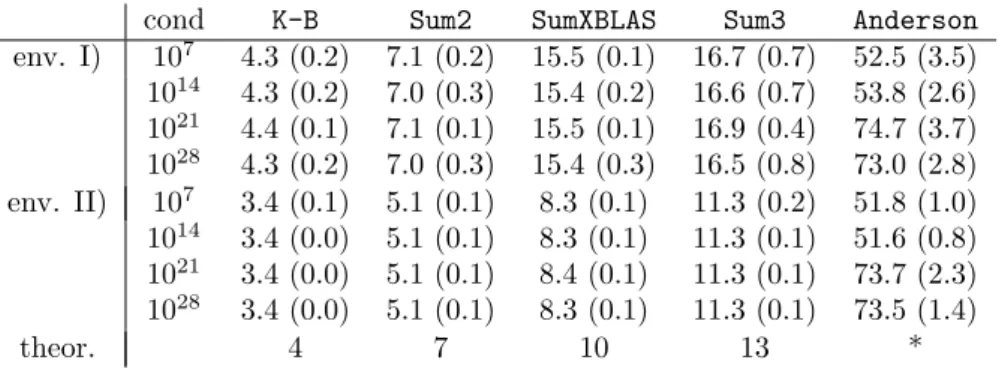
As we will see in a moment, our Algorithm 5.10 (DotK) for K=3 requires the same computing time 37nflops as the XBLAS dot product but delivers a result as if computed in tripled working precision and rounded back into working precision. For IEEE 754 double precision this meansDotK calculates accurate results for condition numbers up to some 1048rather than 1032.
Again it is very instructive to express and interpret our result in terms of the condition number of the dot product. One defines forxTy6= 0,
cond (xTy) := lim ε→0sup ½¯¯ ¯ ¯(x+ ∆x) T(y+ ∆y)−xTy εxTy ¯ ¯ ¯ ¯:|∆x| ≤ε|x|,|∆y| ≤ε|y| ¾ , where absolute value and comparison is to be understood componentwise. A standard computation yields
cond (xTy) = 2|xT| |y|
|xTy| .
(5.7)
Combining this with the estimation in Proposition 5.5 gives the following result.
Corollary 5.7. Let xi, yi ∈F,1 ≤i≤n, be given and denote by res∈F the result computed by Algorithm 5.3 (Dot2). Assume neps<1. Then, if no underflow occurs, ¯ ¯ ¯ ¯res−x Ty xTy ¯ ¯ ¯ ¯≤eps+12γn2cond (xTy). (5.8)
We think this is a most beautiful result. It tells that therelative error of the result of Algorithm 5.3 is not more than a moderate factor timeseps2 times the condition
number plus the relative rounding error unit eps. This is the best we can expect for a result computed in twice the working precision and rounded back into working precision. The factorγ2
nis mainly due to (2.4) which is known to be pessimistic. This
will be confirmed in our computational results in Section 6.
The following algorithm computes an error bound for the dot product in pure floating point. We will prove the error bound to be rigorous, also in the presence of underflow.
Algorithm 5.8. Dot product in twice the working precision with error bound including underflow.
function [res,err] =Dot2Err(x, y)
if 2neps≥1,error(’inclusion failed’),end [p, s] =TwoProduct(x1, y1) e=|s| fori= 2 :n [h, r] =TwoProduct(xi, yi) [p, q] =TwoSum(p, h) t= fl(q+r) s= fl(s+t) e= fl(e+|t|) res= fl(p+s) δ= fl((neps)/(1−2neps))
α= fl(eps|res|+ (δe+ 3eta/eps)) err= fl(α/(1−2eps))
For the proof of validity we use the computed quantitiese,res, δ, αanderrof Algo-rithm 5.8 after execution of the last statement. First note that the quantity in (5.4) is estimated by γn−1 à |s1|+ n X i=2 |fl(qi+ri)| ! ≤(1 +eps)n−1γ n−1fl à |s1|+ n X i=2 |qi+ri| ! ≤ (n−1)eps 1−(2n−2)eps e .
Taking underflow into account and usingres= fl(p+s) it follows
|xTy−res| ≤ eps|res|+|xTy−p−s|+ 5neta
≤ fl(eps|res|) + (n−1)eps
1−(2n−2)eps e+ (5n+ 1)eta =: fl(eps|res|) + ∆. (5.9) Furthermore, (n−1)eps 1−(2n−2)eps≤(1 +eps) −3 neps 1−2neps≤(1 +eps) −2δ
and, using 2neps<1 and regarding possible underflow, ∆≤(1 +eps)−2δe+ (5n+ 1)eta
≤(1 +eps)−1fl(δe) + (5n+ 2)eta
≤(1 +eps)−1(fl(δe) + 3eta/eps)
≤fl(δe+ 3eta/eps). Finally, (5.9) yields
|xTy−res| ≤fl(eps|res|) + fl(δe+ 3eta/eps)≤(1−eps)−1α
≤(1−eps)α/(1−2eps)≤fl(α/(1−2eps)) =err, and proves the following result.
Corollary 5.9. Let xi, yi ∈F, 1≤i≤n, be given and denote by res,err∈F the results computed by Algorithm 5.8(Dot2Err). If Algorithm 5.8 runs to completion, then, also in the presence of underflow,
res−err≤xTy≤res+err.
Algorithm 5.8 requires27n+ 4flops, where taking the absolute value is counted as one flop. If instructions ADD3 andFMAare available, then Algorithm 5.8 can be executed in8n+ 8 flops.
The trick is to move all underflow related constants into eta/eps, the smallest positive normalized floating point number, which vanishes when added to δe except in pathological situations.
Our final step is to extend the idea of the previous algorithm for doubled working precision to higher precision by applying our summation Algorithm 4.8 (SumK).
Algorithm 5.10. Dot product algorithm inK-fold working precision, K≥3.
functionres=DotK(x, y, K) [p, r1] =TwoProduct(x1, y1) fori= 2 :n [h, ri] =TwoProduct(xi, yi) [p, rn+i−1] =TwoSum(p, h) r2n=p res=SumK(r, K−1)
The call of Algorithm 4.8 (SumK) in the last line of Algorithm 5.10 may be replaced by the equivalent Algorithm 4.12 (SumKvert, vertical mode). With our previous results the analysis is not difficult. The error-free transformations TwoProduct (without underflow) andTwoSumyield
s:=
2n
X
i=1
ri=xTy.
To apply Proposition 4.10 we need to estimate S := P2i=1n |ri|. But this is nothing
else than the quantity on the left hand side of (5.3). Inserting this into Proposition 4.10, using 2γm≤γ2mand noting that the vectorris of length 2nyields
|res−xTy| ≤(eps+ 3γ22n−1)|xTy|+γ4Kn−1−2(|xTy|+γ2n|xT| |y|) = (eps+ 3γ2 2n−1+γ4Kn−1−2)|xTy|+γ2nγ4Kn−1−2|xT| |y| ≤(eps+3 4γ 2 4n−2+γ4Kn−1−2)|xTy|+γK4n−2|xT| |y|.
If 4(2n−1)eps≤1, thenγ4n−2≤1 and
|res−xTy| ≤(eps+ 2γ42n−2)|xTy|+γK4n−2|xT| |y|.
(5.10)
The analysis in the presence of underflow is again based on the fact that the only additional error can occur in the initial transformation of the dot productxTy by the
ncalls ofTwoProduct. So (5.10) and Theorem 3.4 prove the following result.
Proposition 5.11. Let xi, yi ∈F, 1≤i≤n, be given and assume 8neps≤1. Denote by res∈F the result of Algorithm 5.10(DotK). Then, in case no underflow occurs, |res−xTy| ≤(eps+ 2γ42n−2)|xTy|+γK4n−2|xT| |y| and ¯ ¯ ¯ ¯res−x Ty xTy ¯ ¯ ¯ ¯≤eps+ 2γ42n−2+ 1 2γ K 4n−2cond (xTy). (5.11)
In the presence of underflow,
|res−xTy| ≤(eps+ 2γ2
4n−2)|xTy|+γ4Kn−2|xT| |y|+ 5neta.
Algorithm 5.10 requires 6K(2n−1) + n + 5 or less than (12K + 1)n flops. If Algorithms 3.6 (TwoSumADD3) and 3.5 (TwoProductFMA) are used instead of Algo-rithms 3.1(TwoSum)and 3.3(TwoProduct), respectively, then Algorithm 5.10 requires
(2K+ 1)(2n−1) flops.
The term 2γ2
4n−2 is negligible against eps. So, as before, this means that the
relative error of the result is essentially the relative rounding error unit epsplus a moderate factor times epsto the K-th power times the condition number. This is again the best we can expect of a computation inK-fold working precision.
Note that Algorithm 5.10 improves the computing time of Algorithm 5.1 from about (12K+ 7)nto (12K+ 1)nflops, whilst satisfying the same error estimate.
6. Numerical results. In this section we present timing and accuracy results. We compare our summation algorithms to ordinary summation, Kahan-Babuˇska, XBLAS and Anderson’s algorithm, and our dot product algorithms to BLAS and XBLAS. All timing was done in Fortran by the first author; some accuracy measure-ments were done in Matlab. All calculations in this section are performed in IEEE 754 double precision as working precision corresponding to about 16 decimal digits.
We will not say much about the many practical applications of our algorithms because i) this is widely known, andii) there are excellent treatments in the recent literature [15, 26]. In the latter, for example, the second chapter consists of sections on “Iterative Refinement of Linear Systems and Least Squares Problems”, on “Avoiding Pivoting in Sparse Gaussian Elimination”, on “Accelerating Iterative Methods for Ax=b, like GMRES”, on “Using Normal Equations Instead ofQRfor Least Squares”, on “Solving Ill-Conditioned Triangular Systems”, on “Eigenvalues and Eigenvectors of Symmetric Matrices” with detailed discussion of the numerical properties and effects and advantages of the use of more accurate dot products (in this case doubled working precision). Everything said over there applies toany algorithm calculating the value of a dot product in doubled working precision, regardless of the method in use, so it applies to our Algorithm 5.3 (Dot2) and, mutatis mutandis, to the higher precision Algorithm 5.10.
To test our algorithms we need extremely ill-conditioned dot products, and a problem is to generate vectorsx, y withfloating point entries causing hundreds of bits cancellation. Ill-conditioned sums of length 2n are generated from dot products of lengthnusing Algorithm 3.3 (TwoProduct) and randomly permuting the summands. For ill-conditioned dot products we designed the following Algorithm 6.1 (GenDot) to generate vectorsx, ywith anticipated condition numberc. We put some effort into this routine to make sure that the vectors are general, not following obvious patterns.
Algorithm 6.1. Generation of extremely ill-conditioned dot products. function [x,y,d,C] = GenDot(n,c)
%
%input n dimension of vectors x,y, n>=6 % c anticipated condition number of x’*y %output x,y generated vectors
% d dot product x’*y rounded to nearest % C actual condition number of x’*y %
%uses r=DotExact(x,y) calculating a floating point number r nearest to x’*y %
n2 = round(n/2); % initialization x = zeros(n,1);
y = x; b = log2(c);
e = round(rand(n2,1)*b/2); % e vector of exponents between 0 and b/2 e(1) = round(b/2)+1; % make sure exponents b/2 and
e(end) = 0; % 0 actually occur in e
x(1:n2) = (2*rand(n2,1)-1).*(2.^e); % generate first half of vectors x,y y(1:n2) = (2*rand(n2,1)-1).*(2.^e);
% for i=n2+1:n and v=1:i, generate x_i, y_i such that (*) x(v)’*y(v) ~ 2^e(i-n2) e = round(linspace(b/2,0,n-n2)); % generate exponents for second half for i=n2+1:n
x(i) = (2*rand-1)*2^e(i-n2); % x_i random with generated exponent y(i) = ((2*rand-1)*2^e(i-n2)-DotExact(x’,y))/x(i); % y_i according to (*) end
index = randperm(n); % generate random permutation for x,y x = x(index); % permute x and y
<