Investigating the Relationship between Exchange
Rate and Inflation Targeting
Siok Kun Sek
School of Mathematical Sciences Universiti Sains Malaysia 11800 Minden, Penang, Malaysia
[email protected] Cheau Pian Ooi
School of Mathematical Sciences Universiti Sains Malaysia 11800 Minden, Penang, Malaysia
Mohd. Tahir Ismail
School of Mathematical Sciences Universiti Sains Malaysia 11800 Minden, Penang, Malaysia
Abstract
This paper conducts empirical investigation on the relationship between exchange rate and inflation targeting regime in the three developed and three emerging Asian economies that have adopted inflation targeting (IT) regime. Using a multivariate GARCH model under BEKK specification, we investigate if exchange rate affect the performance of IT and the performance of IT is compared between Asian and European economies. The comparison is made in terms of changes in economic structure and the disinflation cost. The results show significant correlation between exchange rate movements and inflation and output movements in both sub-periods. IT also has significant impacts on the movements of inflation, output and exchange rate. IT leads to higher volatility in exchange rate movement in majority economies. Comparing the performance of IT across economies, we observe that the volatility in exchange rate has increased dramatically and is very volatile in Asian compared to the developed economies. The decline in inflation impulse is larger in Asian than in developed economies. The implementation of IT does not lead to trade-off of inflation-output in Asia but the trade-off relationship is detected in developed economies.
Keywords: Inflation Targeting, Exchange Rate Flexibility, Multivariate GARCH
1 Introduction
The role of exchange rate in the monetary policy framework in emerging economies is no more a new issue but it still remains a hot topic for debates. Following episodes of crises and the switch of emerging economies from fixed to flexible exchange rate regimes and inflation targeting, the role of exchange rate in the monetary policy framework in emerging markets cannot be ignored. The analysis on the relationship between exchange rate and monetary policy in emerging economies is always characterized by the ‘fear of floating’ behavior claimed by [12]. As discussed in [7], the main reason that emerging economies are fear to float their currencies can be explained by the ‘liability dollarization’. According to this explanation, the debts of emerging economies are denominated in U.S. dollar or foreign currencies. Large fluctuations in exchange rate will have negative effects on their balance sheet stability. Therefore, these economies are reluctant to float the exchange rate freely when the foreign denominated debts increase [9].
Apart from this argument, the relationship between exchange rate and monetary policy framework is closely linked to the theory of “Impossibility of the Holy Trinity”. According to this theory, capital mobility and independence of monetary policy cannot coexist with a fixed exchange rate regime. The middle regime that does not permit fully flexible or fixed regime is not sustainable [6]. [15] argues that intervention of the policymaker in the exchange rate movements may generate two risks: 1) the risk of converting the exchange rate into a nominal anchor that takes over the inflation target; and 2) the risk where the fluctuation of exchange rate may depend on the nature of shocks. On the other hand, [4] argues that targeting the exchange rate under inflation targeting regime may cause the loss of credibility in the policy.
In this paper, we seek to explore the inter-relationship between exchange rate flexibility/ regime and the performance of inflation targeting between two groups of economies, i.e. the emerging economies of Asia and the developed economies. In particular, we seek to answer questions such as with the intervention of the policymaker in the exchange rate movement, can inflation targeting work well in emerging market? Does inflation targeting perform better compare to the rigid exchange rate regime in the pre-crisis period? Are the results differ across two groups of economies?
In order to answer these questions, this study empirically investigates the relationship between exchange rate and inflation targeting regime in six economies i.e. three developed economies (Norway, Sweden and United Kingdom (U.K.)) and three Asian economies (Korea, Philippines and Thailand) for pre-IT and post-IT period. Although these Asian economies were reluctant to leave their currencies to float freely before the crisis between 1997 and 1998, shifting their monetary framework to inflation targeting may have changed their response to the
exchange rate. We are interested in seeking how the monetary policy responds to the exchange rate and inflation targeting regimes adopted after the crisis.
The rest of the paper is organized as follows: Section 2 is the literature review on the link between the exchange rate and inflation targeting regime. Section 3 is about data and methodology. Section 4 discusses the results of estimation and diagnostics tests. Finally, the last section concludes.
2 Literature review
The inter-relationship between exchange rate and monetary policy of IT can be examined in three main issues as discussed in [2]. These issues are 1) exchange rate pass-through and the role of exchange rate as shock absorber; 2) exchange rate volatility and IT and 3) exchange rate and policy reaction function. Exchange rate pass-through is defined as the percentage change in the domestic or imported prices led by a one percentage change in the exchange rate between the importer and exporter currency. Pass-through is said to be completed if the effect of the depreciation is fully reflected in import prices. If only a portion of the depreciation is reflected in import prices, then the pass-through is described as partial or incomplete.
Based on the concept of exchange rate pass-through, [4] argues that IT regime induces lower pass-through due to strong commitment to achieve price stability. Lower exchange rate pass-through, in turn, stimulates low inflationary impulse. Taylor’s view is supported by many empirical studies e.g. [11], [10] and [5]. However, [2] argues that the pass-through problem does not only affect inflation alone, it is also related to the effectiveness role played by exchange rate as a shock absorber. [2] extends the concept of effectiveness nominal exchange rate as a shock absorber in inflation targeting regime. The role of exchange rate as a shock absorber can be illustrated by distinguishing the pass-through of exchange rate changes into the price of nontradables and tradables. A high pass through for nontradables will reduce the effectiveness of the nominal exchange rate while a high pass through for tradables will enhance its effectiveness. In other word, exchange rate will act as an effective shock absorber if pass-through into domestic prices leads to depreciation in real exchange rates, hence expenditure switching effect.
The relationship between inflation targeting regime and exchange rate regime has led some analysts to conclude that one of the costs of inflation targeting adoption is the increase in exchange rate volatility. Yet, some studies show that the adoption of a free-floating exchange rate does not necessarily implies more effective of nominal and real exchange rate floating. [22] argue that inflation targeting would lead to higher exchange rate volatility. [12] find that the lack of credibility of monetary authority may lead to exchange rate volatility problem. These authors argue that many emerging countries that officially announce themselves to be free floaters are in fact managed exchange rate regimes. This problem is known as fear of floating. The reason is they reluctant to allow their
currencies to float. Under those circumstances, the monetary authority is likely to place additional constraint on emerging market countries’ monetary policy by smoothing the exchange rate floating.
However, based on the study in Chile, [17] indicate that the volatility of nominal exchange rates of inflation targeting countries does not increase compare to other countries with floating exchange rate regimes. The recent study by [2] on seven countries with some extensions to Chile shows that inflation targeting does not result in an increase in exchange rate volatility. Yet the author emphasizes that inflation targeting helps reduce unexpected shocks by making monetary policy transparent and predictable.
The role of exchange rate in the design of monetary policy rules is another way to study the relationship of exchange rate and monetary policy. It is important to distinguish whether the exchange rate matters to the extent that it is relevant for domestic inflation, or monetary authorities care about the exchange rate for reasons other than inflation.
[1] discusses the reasons for monetary policy to react to exchange rate: 1) monetary policy rule with the exchange rate term may affect the total effects of policy adjustment on economy; 2) this augmented rule improves the effectiveness in the adjustment of interest rate and exchange rate effects on inflationary impulse; 3) it helps to stabilize the effects of real shocks which led by the exchange rate misalignment.
On the other hand, some economists and researchers have different views about the role of exchange rate in the formation of monetary policy rule in emerging economies. According to [4], exchange rate has indirect impact on inflation and output in the policy reaction function and there is no need to include the exchange rate term in the policy reaction function. Besides, Taylor also argues that deviation of exchange rate from purchasing power parity should not be offset through interest rate adjustments as the adjustment may induce negative impacts on real output and inflation. Exchange rate movements reflect real shocks, such as productivity and terms of trade. As a result, it is better not to respond to the exchange rate. In addition, under an inflation-targeting regime, targeting the exchange rate may cause the loss of credibility in targeting inflation.
In contrast, empirical findings report quite different results. For instance, [8] in their study on six Central and Eastern European countries find that during the fixed exchange rate regimes periods, exchange rate plays an important role in the monetary policy. However, the influence disappears after these countries have moved to the flexible regimes. Contrary view, [3] in his study on three Asian inflation targeting countries finds no evidence of monetary policy responds to the exchange rate.
3 Methodology
For the purpose of analysis, a multivariate GARCH (1,1) model with BEKK specification is applied. Consider a vector stochastic process
{ }
yt with1
N× dimension. Let It−1, denote the past information set generated by the observed series
{ }
yt until time t−1. According to [13],{ }
yt is represented by(1) yt =μ εt+ t,
(2) 12
t H zt t
ε = where μt is the conditional mean vector N×1 vector, 12
t
H is the positive definite matrix (N×N), zt is iid vector N×N, it is assumed that the N×1 vector zt to has the following first two moment:
( )
t 0 E z = and( )
var zt =IN
where IN is the identity matrix of order N. The GARCH (1, 1) is the simplest and most robust among the family of volatility models. In GARCH (1, 1), we calculate the long-run average variance rate, VL, and also the lag terms of σn−1 and εn−1 in order to obtain conditional variance matrix (Su & Huang, 2010). The equation of the conditional variance for GARCH (1, 1) is represented by:
(3) σn2 =γVL+αεn2−1+βσn2−1
where γ is the weight assigned to VL, α is the weight assigned to 2 1
n
ε − , and β is the weight assigned to σn2−1. The weights are sum to one, that is,
(4) γ α β+ + =1. This BEKK model was suggested by [21] in a preliminary version of [16]. The main feature is that it does not need any restriction on parameters to get positive definiteness of the Ht matrix. This is due to the general quadratic structure of the
model. The fundamental BEKK-GARCH model can be written as:
(5) Ht =CC'+
∑ ∑
qj=1 kK=1Akj'ε εt j− t'−jAkj +∑ ∑
pj=1 Kk=1B Hkj' t j− Bkj where C, Akj and Bkj are n n× matrices of parameters but C is an upper triangular matrix. The positive definiteness of the variance covariance matrix is controlled by the constant matrix CC .' The parameters are estimated using the quasi-maximum likelihood procedure of [14]. { }εt is covariance stationarity if anonly if the modulus of all eigenvalues of A⊗ + ⊗A B B are smaller than unity ([19]. As discussed in [20], the (quasi) log likelihood function of the multivariate GARCH model is expressed by:
(6) log
(
(
1)
)
log 2( )
1log 1 ' 12 2 2
t t t t t
K
f ε Ω− Σ = − π − Σ − εΣ−ε For the purpose of our study, we use BEKK model to investigate: (1) the
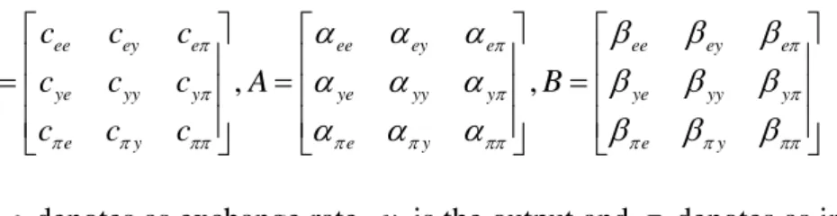
correlations between the three variables i.e. exchange rate, industrial production index and inflation rate; (2) the impact of shock for past value; and (3) the persistency of the three variables to economy. Therefore the matrices of C, A
, , ee ey e ee ey e ee ey e ye yy y ye yy y ye yy y e y e y e y c c c C c c c A B c c c π π π π π π π π ππ π π ππ π π ππ α α α β β β α α α β β β α α α β β β ⎡ ⎤ ⎡ ⎤ ⎡ ⎤ ⎢ ⎥ ⎢ ⎥ ⎢ ⎥ =⎢ ⎥ =⎢ ⎥ =⎢ ⎥ ⎢ ⎥ ⎢ ⎥ ⎢ ⎥ ⎣ ⎦ ⎣ ⎦ ⎣ ⎦
where the e denotes as exchange rate, y is the output and π denotes as inflation. The lower triangular of C is equal to zero in our study.
4 Data
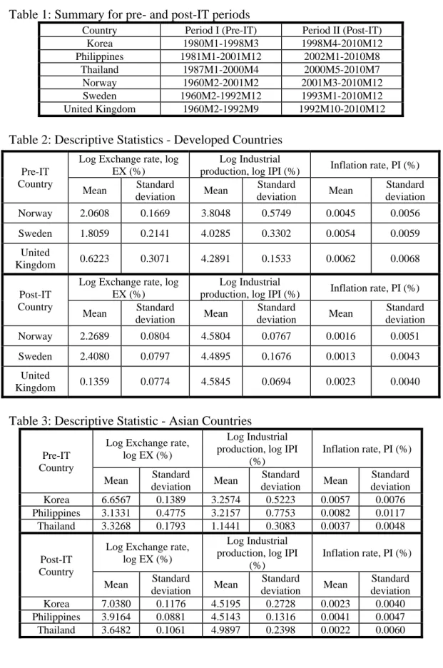
This study extends the previous study by [19] in examining the inter-relationship between monetary policy of inflation targeting and exchange rate in several emerging economies in Asia. The Asian economies that included in this study are Korea, Philippines and Thailand while the developed economies included are Norway, Sweden and U.K. These economies have adopted the inflation targeting regime at different time i.e. Korea in April 1998, Thailand in May 2000, Philippines in January 2002, Norway in March 2001, Sweden in January 1993 and U.K. in October 1992. The data are divided into two sub-periods – before and after the adoption of IT. The full sample series are from 1960M1 to 2010M12. Table 1 summarizes the ranges of pre- and post-IT periods for these six economies.
The data are in monthly and are collected from the International Financial Statistics (IFS) 2011 in International Money Fund (IMF). These data include nominal national local currency per USD exchange rate (average of the month) as proxy of exchange rate (EX), industrial production index (IPI) to proxy the output variable and consumer price index (CPI) is used to construct inflation rate (PI). Inflation is constructed by finding the difference between price levels for the current month and previous given month, i.e. πt =log(CPIt) log(− CPIt−1). Output and inflation are indicators used to measure the performance of inflation targeting. The objective of inflation targeting is to achieve stability in output growth and low inflation rate. The analysis on the inter-relationship of exchange rate, output and inflation suppose to provide better understanding on the link between exchange rate flexibility/ regime and the performance of inflation targeting.
Table 2 and 3 summarize the descriptive statistics for these three variables in log form (or in %). As observed, exchange rate is more volatile/ flexible under the implementation of IT. Besides, the output growth has increased while inflation rate has declined in the post-IT periods in all economies. Does the data indicate that IT works well in all economies? Does the change in the exchange rate flexibility have impact on the performance of IT? We explore the analysis in the next section.
Table 1: Summary for pre- and post-IT periods
Country Period I (Pre-IT) Period II (Post-IT)
Korea 1980M1-1998M3 1998M4-2010M12 Philippines 1981M1-2001M12 2002M1-2010M8 Thailand 1987M1-2000M4 2000M5-2010M7 Norway 1960M2-2001M2 2001M3-2010M12 Sweden 1960M2-1992M12 1993M1-2010M12 United Kingdom 1960M2-1992M9 1992M10-2010M12
Table 2:Descriptive Statistics - Developed Countries
Table 3: Descriptive Statistic - Asian Countries
Pre-IT Country
Log Exchange rate, log EX (%)
Log Industrial production, log IPI
(%) Inflation rate, PI (%) Mean Standard deviation Mean Standard deviation Mean Standard deviation Korea 6.6567 0.1389 3.2574 0.5223 0.0057 0.0076 Philippines 3.1331 0.4775 3.2157 0.7753 0.0082 0.0117 Thailand 3.3268 0.1793 1.1441 0.3083 0.0037 0.0048 Post-IT Country
Log Exchange rate, log EX (%)
Log Industrial production, log IPI
(%) Inflation rate, PI (%) Mean Standard deviation Mean Standard deviation Mean Standard deviation Korea 7.0380 0.1176 4.5195 0.2728 0.0023 0.0040 Philippines 3.9164 0.0881 4.5143 0.1316 0.0041 0.0047 Thailand 3.6482 0.1061 4.9897 0.2398 0.0022 0.0060 Pre-IT Country
Log Exchange rate, log EX (%)
Log Industrial
production, log IPI (%) Inflation rate, PI (%) Mean Standard deviation Mean Standard deviation Mean Standard deviation Norway 2.0608 0.1669 3.8048 0.5749 0.0045 0.0056 Sweden 1.8059 0.2141 4.0285 0.3302 0.0054 0.0059 United Kingdom 0.6223 0.3071 4.2891 0.1533 0.0062 0.0068 Post-IT Country
Log Exchange rate, log EX (%)
Log Industrial
production, log IPI (%) Inflation rate, PI (%) Mean Standard deviation Mean Standard deviation Mean Standard deviation Norway 2.2689 0.0804 4.5804 0.0767 0.0016 0.0051 Sweden 2.4080 0.0797 4.4895 0.1676 0.0013 0.0043 United Kingdom 0.1359 0.0774 4.5845 0.0694 0.0023 0.0040
5 Results and Discussions
The results of multivariate GARCH (1,1) are summarized in Table 4 to 7 in appendix. *** denotes the result is significant at 1% level while ** and * denote the significance results at 5% and 10% levels respectively. The values shown in brackets are t-values. C is the coefficient matrix that summarizes the mean of the conditional variances or covariance. The diagonal coefficients show the means conditional variances of exchange rate, output growth and inflation respectively while the off diagonal coefficients are their means covariance. We observe that the mean conditional variance for inflation rate is very small while the mean conditional variance for exchange rate is the largest among the three means conditional variance. This condition holds for all economies except the case of U.K. in which the mean conditional variance for output has the largest value.
Comparing the results across economies, we observe that the mean conditional variance of exchange rate is much larger than the one in developed economies regardless the pre- or post-IT periods. Comparing the results between the two sub-periods, the results reveal that the means conditional covariance of exchange rate-inflation and output-rate-inflation are weak and not significant in the post-IT periods in most cases. However, the mean conditional covariance of exchange rate-output is significant and has increased in the post-IT period in general.
A is the ARCH coefficient matrix. The diagonal coefficients show the correlation between the conditional variance of variables with their past squared errors or past information while the off-diagonal elements indicate the link between the past information or squared error of one variable and the conditional variance of another variable. The first column of this matrix shows the impact of past information or past squared errors of exchange rate on the current conditional variance of exchange rate, output and inflation. The impact of exchange rate on inflation is weak and insignificant after the implementation of IT in all cases. In overall, we can say that exchange rate has some impacts on the economic variables in both sub-periods. However, its impact on inflation is insignificant in the post-IT period. The impacts vary across economies. In turn, the conditional variance of exchange rate is determined significantly by past squared error of inflation in both sub-periods in all economies (except U.K. in the post-IT period). Both past squared errors of inflation and conditional variance of exchange rate has positively correlated in the pre-IT period in all Asian economies but the correlation changes to negative in the post-IT period. This means that an increase in one percent past squared error of inflation will reduce the exchange rate volatility in the post-IT period and this leads to lower inflation. In developed economies, the correlation is mixed. In general, the past squared errors of inflation also have impacts on output and inflation. The correlation is changing from negative to positive in the case of Asia. The results imply that an increase in one percent in past-squared error of inflation leads to an increase of output in Asia after the adoption of IT rather than reducing the output in the pre-IT period. The results imply the news of lower inflation leads to higher growth in the pre-IT
period compared to the negative impact of lower inflation news on the output growth, i.e. lower inflation news leads to lower growth in the post-IT periods. In developed economies, we detect negative impact of inflation on output growth in Norway and Sweden but the impact is positive in U.K. after the adoption of IT. Overall, we can say that inflation has effectively changed the economic structure of these economies in the post-IT period.
We also observe that the mean conditional variance of inflation has declined, implying lower inflation rate in the post-IT period. The news of lower inflation may require greater exchange rate adjustment/ flexibility to smooth down shocks. Hence, it is reasonable to observe that the past information of inflation is negatively linked to the conditional variance of exchange rate in the post-IT period in majority economies. On the other hand, there are evidences that past information of lower inflation rate induces lower growth in the post-IT period. This is possible because lower price level leads to lower motivation for producer to increase their production.
B is the coefficient matrix that indicates the relationship between current conditional variance of variables and their past conditional variances. The diagonal elements show the persistency in the conditional variance. The off-diagonal elements on the other hand, show the correlation between the conditional variance of one variable and the past conditional variance of another variable. This coefficient matrix provides information on the analysis of trade-off relationship between inflation and output variable. By observing the last column of this matrix, the results of second row reveal the trade-off relationship between inflation and output growth.
Comparing the results across economies, we observe that the results vary across economies. Persistency of exchange rate in Thailand is the highest among the Asian countries while it is the lowest in Philippines. Overall, the persistency of exchange rate, output and inflation of the entire countries do not exhibit significant changes between the two sub-periods.
The past conditional variance of exchange rate is linked positively to the conditional variance of output in Philippines, Norway, Sweden and U.K. in the pre-IT period and Thailand and U.K. in the post-IT period. Its impact is positively significant on the conditional variance of inflation in Thailand, Norway and U.K. in the pre-IT period but not significant after the adoption of IT in all countries. The past conditional variance of inflation has positive significant impact on the current conditional variance of output in three Asian economies. The impact changes to negative after the adoption of IT. The results imply a trade-off relationship between inflation and output in the pre-IT period but the trade-off relationship disappears in the post-IT period. In developed economies we observe positive or trade-off relationship in Norway but negative relationship is observed in Sweden and U.K. in the pre-IT period. We only observe negative significant impact of past conditional of variance on conditional variance of output in Sweden after the adoption of IT.
The past conditional variance of output in turn, also has impact on the conditional variance of inflation. The impact is significant in some Asian
economies before and after the implementation of IT. On the other hand, the impact is not significant in all developed economies after the adoption of IT. In overall, we say that IT does not induce disinflation cost in Asian economies but the trade-off relationship in inflation-output is detected in the developed economies. The implementation of IT induces changes in the relationship between inflation and output growth which varies across economies.
6 Conclusions
This paper conducts empirical analysis on the relationship between exchange rate flexibility/ regime and monetary policy of inflation targeting in several emerging and developed economies. Applying a multivariate GARCH model, the results show significant correlation between exchange rate movements and inflation and output movements in both sub-periods. IT also has significant impacts on the movements of inflation, output and exchange rate. IT is associated with higher volatility in exchange rate movement in majority economies. Comparing the performance of IT across economies, we observe that the volatility in exchange rate has increased dramatically and it is very volatile in emerging Asia compare to the developed economies. The decline in inflation impulse is larger in emerging Asia than in developed economies. The implementation of IT does not lead to the trade-off of inflation-output in Asia but the trade-off relationship is detected in developed economies. We can say that IT has effectively in lowered the inflation rate and boost up the emerging economies in Asia compared to the developed economies.
References
[1] B. J. Eichengreen, and R. Hausmann, Debt denomination and financial instability in emerging market economies, Manuscript, UC Berkeley, 2003. [2] E. U. Choudhri, and D. S. Hakura, Exchange rate pass-through to domestic
prices: does the inflationary environment matter? Journal of International Money and Finance, 25 (2006), 614-639.
[3] F. S. Mishkin, Can Inflation Targeting Work in Emerging Market Countries? NBER Working Papers 10646, National Bureau of Economic Research, Inc, 2004.
[4] G. A. Calvo, and C. M. Reinhart, Fear of floating, Quarterly Journal of Economics, 117(2) (2002), 379-408.
[5] H, Herwartz, Conditional heteroskedasticity, In: H. Lütkepohl and M. Krätzig, Applied time series econometrics, Cambridge University Press, (2004) 197-220.
[6] J. B. Taylor, The role of the exchange rate in monetary policy rules, American Economic Review, 91(2) (2001), 263-267.
[7] J. E. Gagnon, and J. Ihrig, Monetary policy and exchange rate pass-through, Board of Governors of the Federal Reserve System, Washington, 2004. [8] J. Gali, and T. Monacelli, Monetary policy and exchange rate volatility in a
small open economy, The Review of Economic Studies, 72(3) (2005), 707-734.
[9] J. M. Campa, and L. S. Goldberg, Exchange rate pass-through into import prices: a macro or micro phenomenon? NBER working paper, 2002.
[10] K. Schmidt-Hebbel, and M. Tapia, Monetary Policy Implementation and Results in Twenty Inflation-Targeting Countries, Working Papers Central Bank of Chile 166, Central Bank of Chile, 2002.
[11] L. Bauwens, S. Laurent, and J. V. K. Rombouts, Multivariate GARCH models: A Survey, Journal of Applied Econometrics, 21(1) (2006), 79-109. [12] M. Adolfson, Incomplete exchange rate pass-through and simple monetary
policy Rules, Journal of International Money and Finance, 26 (2007), 468-494.
[13] M. Frömmel, and F. Schobert, Monetary policy rules in Central and Eastern Europe, Universität Hannover and Deutsche Bundesbank, Discussion paper no. 341, 2006.
[14] M. Karanasos, and J. Kim, The inflation-output variability relationship in the G3: a bivariate GARCH (BEKK) approach, Risk Letters, 1(2) (2005), 17-22.
[15] N. Osawa, Monetary policy responses to the exchange rate: empirical evidence from three East Asian inflation targeting countries, Bank of Japan working paper series no. 06-E-14, 2006.
[16] R. F. Engle, and F. K. Kroner, Multivariate simultaneous generalized ARCH, Econometric Theory, 11 (1995), 122-150.
[17] R. Hausmann, U. Panizza, and R. Rigobon, The long run volatility puzzle of the real exchange rate, NBER working paper no. 10751, 2004.
[18] S. Edwards, The relationship between exchange rates and inflation targeting Revisited, NBER working paper series no. 12163, 2006.
[19] T. Bollerslev, R. F. Engle, and J. M. Wooldridge, A capital asset pricing model with time varying covariances, Journal of Political Economy, 96
(1988), 116-131.
[20] T. Cavoli, and R. Rajan, Designing appropriate exchange rate regimes for East Asia: inflation targeting and monetary policy rules, University of Adelaide, Discussion paper no. 0309, 2003.
[21] W. J. Su, and Y. Y. Huang, Comparison of Multivariate GARCH Models with Application to Zero-Coupon Bond Volatility, Master thesis, University of Lund, 2010.
[22] Y. Baba, R.F. Engle, D.F Kraft, and K.F. Kroner, Multivariate Simultaneous Generalized ARCH, Department of Economics Mimeo, University of California, San Diego, 1990.
Appendix
Table 4:Estimation results for Asian economies - pre- IT period
Country Coefficient C A B e y π e y π e y π Korea e 1.4888*** (-8.9184) 0.7292*** (-6.4727) 0.0013 (-0.0490) 0.2236*** (3.00589) -0.0300 (-0.8052) 0.0300 *** (77.3540) 0.9487*** (60.7775) 0.0300*** (3.8816) -0.0300*** (24.0597) y 0.0000 (0.0000) 0.1116*** (-3.9286) -0.0004 (-0.0359) -0.0300 (-0.3498) 0.2236*** (5.0483) -0.0300*** (-48.6313) 0.0300 (1.0327) 0.9487*** (68.1879) 0.0300*** (12.6812) π 0.0000 (0.0000) 0.0000 (0.0000) 0.0023*** (-6.5401) -0.0297 (-0.0078) 0.0302 (0.0199) 0.2235*** (10.3904) -0.0300 (0.9456) 0.0300** (2.1689) 0.9487*** (332.1802) Phil. e 0.8670*** (5.1191) 0.8632*** (5.2128) 0.0068*** (5.4566) 0.9080*** (5.8449) 0.6371*** (3.9816) 0.0356*** (22.4562) 0.5146*** (5.6614) -0.369*** (-4.6443) -0.032*** (-8.4853) y 0.0000 (0.0000) 0.0917*** (9.5127) -0.0041 (-0.5990) -0.7376*** (-4.4582) -0.4688*** (-2.7869) -0.0363*** (-25.3528) 0.4432*** (4.5965) 1.3289*** (16.0146) 0.0320*** (7.6303) π 0.0000 (0.0000) 0.0000 (0.0000) -0.0001** (-2.2104) 0.1134 (0.0582) -0.0043 (-0.0024) 0.2294*** (2.6478) -1.1600 (-1.1268) -1.1969 (-1.1250) 0.9471*** (83.4202) Thai. e 0.7851*** (3.000) 0.9731*** (2.8011) 0.0082 (1.4161) 0.3058 (1.1634) 0.0612 (0.1995) 0.0419*** (4.5995) 1.0178*** (20.453) 0.1009* (1.6871) 0.0320*** (-9.1805) y 0.0000 (0.0000) 0.0587*** (2.6587) 0.0104** (-2.3870) -0.0379 (-0.1870) 0.2174 (0.9008) -0.0396*** (-5.2915) -0.0500 (-1.1152) 0.8653*** (15.8966) 0.0307*** (10.6792) π 0.0000 (0.0000) 0.0000 (0.0000) -0.0002 (-1.5753) -10.159*** (-3.0513) -11.502** (-2.5350) 0.0250 (0.1396) 0.2991*** (3.0939) 0.3468** (2.3314) 0.9503*** (41.1768)
Table 5:Estimation results for Asian economies - post- IT period Country Coefficient C A B e y π e y π e y π Korea e 1.5740*** (9.9541) 1.0100*** (9.6326) 0.0005 (0.0237) 0.2236 *** (2.8897) -0.0300 (-0.6551) -0.0300*** (-16.8181) 0.9487*** (18.5682) 0.0300 (1.2903) 0.0300*** (4.4620) y 0.0000 (0.0000) 0.0071* (1.8379) 0.000008 (0.0041) -0.0300 (-0.2912) 0.2236*** (3.5070) 0.0300*** (11.2119) 0.0300 (0.3858) 0.9487*** (27.4719) -0.0300*** (-2.8107) π 0.0000 (0.0000) 0.0000 (0.0000) 0.0009 *** (5.4800) -0.0300 (-0.0041) 0.0300 (0.0066) 0.2236*** (3.1051) 0.0300 (0.2961) -0.0300 (-0.6074) 0.9487*** (74.9753) Phil. e 1.0706*** (2.8897) 1.2115*** (2.9403) -0.0045 (-0.5126) 0.7705 (0.9830) 0.5670 (0.6667) -0.0308*** (-3.4710) 0.8733*** (3.4289) -0.05049 (-0.1765) 0.0300*** (2.8014) y 0.0000 (0.0000) 0.0478*** (4.5291) 0.0032 (0.7498) -0.5057 (-0.7504) -0.2947 (-0.4024) 0.0313*** (3.9553) 0.0832 (0.3522) 1.0051*** (3.7523) -0.0295*** (-2.9313) π 0.0000 (0.0000) 0.0000 (0.0000) -0.0001*** (-4.7403) 5.1624 (0.6030) 5.8194 (0.6013) 0.1983 (1.6116) -0.4886 (-1.4501) -0.5256* (-1.6628) 0.9536*** (54.5974) Thai e 0.7159** (2.1564) 0.9113** (2.0215) -0.0246* (-1.8738) 0.9932*** (13.426) 0.9327*** (10.608) -0.0846*** (-9.9702) 0.7512*** (18.9701) -0.1874** (-2.2939) 0.0559*** (3.0161) y 0.0000 (0.0000) 0.1338*** (3.0281) 0.0161 (0.7790) -0.5043*** (-7.6766) -0.3669*** (-4.7467) 0.0692*** (9.5907) 0.1293*** (4.1722) 1.0543*** ( 15.8199) -0.0463*** (-3.1528) π 0.0000 (0.0000) 0.0000 (0.0000) 0.0006*** (2.9029) 3.1365 (0.5986) 3.2902 (0.4433) -0.3840*** (-5.0171) -0.9653 (-0.0230) -1.2015*** (-8.2183) 1.0016*** (25.9753)
Table 6:Estimation results for developed economies - pre- IT period Country Coefficient C A B e y π e y π e y π Korea e 0.4707*** (9.5545) 0.8390*** (6.1967) 0.0050 (0.2530) 0.3761*** (4.4681) 0.1842* (1.6684) 0.0479*** (4.9829) 0.9555*** (112.5169) 0.0420 (1.1047) -0.0267** (-2.3735) y 0.0000 (0.0000) 0.1013*** (3.3495) -0.0001 (-0.0126) -0.0925** (-1.9888) 0.1520** (2.5017) -0.0413*** (-7.9297) 0.0127* (1.7389) 0.9199*** (28.8998) 0.0260*** (3.4571) π 0.0000 (0.0000) 0.0000 (0.0000) 0.0003*** (11.0247) -2.2775** (-2.4142) -3.0300 (-1.1642) -0.2105 (-0.6812) 0.0448* (1.8500) 0.1941*** (4.8686) 0.9423*** (67.4879) Phil. e 0.4067*** (7.0100) 0.8987*** (8.6904) 0.0012 (0.0775) 0.2236*** (2.7783) -0.0300 (-0.2337) -0.0300** (-2.1522) 0.9487*** (53.7426) 0.0300 (0.9994) 0.0300*** (5.3130) y 0.0000 (0.0000) 0.0963** (2.0061) 0.0002 (0.0229) -0.0300 (-0.8158) 0.2236*** (3.6360) 0.0300*** (4.8439) 0.0300*** (3.7717) 0.9487*** (60.3136) -0.0300*** (10.4807) π 0.0000 (0.0000) 0.0000 (0.0000) 0.0008*** (2.6008) -0.0302 (0.0390) 0.0298 (0.0128) 0.2237 (0.9750) 0.0300 (1.2447) -0.0300 (0.8856) 0.9487*** (119.6702) Thai e 0.1553*** (4.3200) 0.8480*** (12.9858) 0.0012 (0.0308) 0.2236*** (8.8912) -0.0300 (-0.2722) -0.0300*** (-3.8562) 0.9487*** (132.913) 0.0300*** (4.5036) 0.0300*** (5.1837) y 0.0000 (0.0000) 0.4493*** (5.4958) 0.0007 (0.0829) -0.0300*** (-15.219) 0.2236 *** (31.2929) 0.0300*** (18.2236) 0.0300*** (17.4906) 0.9487*** (241.261) -0.0300*** (-14.9052) π 0.0000 (0.0000) 0.0000 (0.0000) 0.0007*** (11.074) -0.0300 (-0.0652) -0.0300 (-0.0168) 0.2236 (0.8212) 0.0300** (2.9097) 0.0300*** (3.2125) 0.9487*** (98.3512)
Table 7:Estimation results for developed economies - post- IT period Country Coefficient C A B e y π e y π e y π Korea e 0.5077** (2.0572) (1.4183) 1.0238 (0.0043) 0.0003 (0.3317) 0.2236 (-0.0275) -0.0300 -0.0300** (-1.9749) 0.9487*** (10.0792) (0.0239) 0.0300 (0.0714) 0.0300 y 0.0000 (0.0000) 0.0343 (0.0535) 0.0002 (0.0012) -0.0300 (-0.0783) 0.2236 (0.3448) 0.0300*** ( 3.5209) 0.0300 (0.6675) 0.9487 (1.5127) -0.0300 (-0.1435) π 0.0000 (0.0000) 0.0000 (0.0000) 0.0011 (0.6623) -0.0300 (-0.0053) -0.0300 (-0.0026) 0.2236 (1.12082) 0.0300 (0.2097) -0.0300 (-0.0158) 0.9487 (1.5022) Phil. e 0.5387*** (5.6360) 1.0034*** (5.10241) 0.0003 (0.0332) 0.2236* (1.6818) -0.0300 (-0.1350) -0.0300*** (-24.9847) 0.9487*** (18.7616) 0.0300 (0.4735) 0.0300*** (44.9045) y 0.0000 (0.00000) 0.0497 (0.83632) 0.0002 (0.0761) -0.0300 (-0.3751) 0.2236** (1.9701) 0.0300*** (44.5785) 0.0300 (1.0671) 0.9487*** (26.71744) -0.0300*** (-86.1350) π 0.0000 (0.00000) 0.0000 (0.00000) 0.0009 (0.8646) 0.0300 (0.0074) -0.0300 (-0.0040) 0.2236*** (35.5416) 0.0300 (0.4462) -0.0300 (-0.3836) 0.9487*** (443.9801) Thai. e 0.0350 (0.43139) 0.8946*** (10.34025) 0.0005 (0.0075) 0.2236*** (3.14294) -0.0300 (-0.0450) 0.0300 (1.4650) 0.9487*** (7.2287) -0.0300 (-0.04971) -0.0300 (-0.2219) y 0.0000 (0.00000) 0.5008* (1.76084) 0.0002 (0.0129) -0.0300*** (-30.8716) 0.2236*** (7.1606) -0.0300*** (-27.9495) 0.0300*** (7.3456) 0.9487*** (42.3654) 0.0300*** (8.5436) π 0.0000 (0.00000) 0.0000 (0.00000) 0.0009 (1.6084) 0.00300 (0.1514) -0.0300 (-0.0064) 0.2236*** (5.5233) -0.0300 (-0.1798) -0.0300 (-0.0396) 0.9487*** (5.4609) Received: September, 2011