Is Effect of Macroprudential Policy Frequency-Specific? A Design Limit Approach

(1)

A Design Limit Approach

∗

Junghwan Mok† Myungkyu Shim‡

November 23, 2015

Abstract

Do macroprudential policies effectively stabilize aggregate economy at every frequency? In order to answer to this question, this paper uses an extended New Keynesian model with a financial sector to analyze if different sets of macroprudential policies, which are commonly considered in the literature and practice, are successful in stabilizing goods and financial markets at different frequencies. Our findings indicate that those well-known policies are successful in stabilizing financial markets, but at substantial costs of amplifying fluctuations in real sectors; the loan fluctuations are reduced almost at every frequency under most policies. However, the output fluctuations are amplified almost at every frequency (2 to 24 years) under any policies. In other words, our finding raises the importance of studying carefully designed macroprudential policies to minimize such an adverse effect, which is the design limit of current policies in the sense that they are effective in the designated markets and frequencies while have perverse effects at other markets and frequencies.

∗

First Draft: Sep, 2015. This Draft: Nov, 2015. Myungkyu Shim gratefully acknowledges financial support from the Bank of Korea. The views in this paper are those of the authors, and do not necessarily reflect those of the Bank of Korea. We are grateful to Soyoung Kim and Jinil Kim for their helpful comments and suggestions. We would also like to thank seminar participants at Bank of Korea.

†

Financial Stability Department, Bank of Korea. Email: [email protected] ‡

(2)

1 Introduction

Attention to policies whose goals are stabilizing financial sector has greatly increased aftermath of the Great Recession, which is considered as the most severe recession since 1950s and is initiated from the collapse of the financial market. The effectiveness of a traditional monetary policy, Taylor rule for instance, is limited in such a situation since it is designed to stabilize output and inflation at the business cycle frequency (1.5 years to 8 years), but not to stabilize the financial market. As a result, literature has instead focused on the role of macroprudential policy, which is designed to “strengthen the financial system’s resilience to economic downturns and other adverse aggregate shocks and actively limit the build-up of financial risks” (BIS (2010)). Since the financial cycle is believed to have a much lower frequency (usually upto 16 years per cycle) than the usual business cycle has (Borio (2012)), the macroprudential policy usually aims to lower the volatility of the macroeconomy relatively at the low frequency. Hence, asking the effectiveness of such a policy can be translated into the question if the policy achieves its objective in lowering variance at the designated (low) frequency.

This paper is in line with the existing literature in the sense that we study the effectiveness of macro-prudential policy within a business cycle model with a financial sector. The conventional method to evaluate the performances of policies adopted by the previous literature is the “welfare-cost” approach; they compute the value of lifetime utility under different policy regimes and compare them using the compensational variation in terms of consumption.1 One stream of literature focuses on measuring the welfare cost of policies. Van Den Heuvel (2008) measures the welfare cost of bank capital requirement and shows the regulation produces 0.1% to 1% loss in consumption in the U.S economy. Nguyen(2014) uses a general equilibrium model with a dynamic banking sector to show the increase of bank capital requirement to the optimal level can produce welfare gains greater than 1% of lifetime consumption.

Another stream of literature tries to answer in which situations macroprudential policies are effective. Benes and Kumhof(2015) shows the countercyclical bank capital requirement can creates a precautionary motive to banks when the creditworthiness (or riskiness) of borrowers depreciates. Bailliu, Meh, and Zhang(2015) compares different sets of macroprudential regimes and finds that welfare gain is the largest when macroprudential policies reacts to the financial shocks rather than productivity shocks. Lastly, a group of literature search for the optimal coordination between monetary and macroprudential policies. Quint and Rabanal(2014) andSuh(2012) find the optimal simple rule for monetary and macroprudential policies in the Euro Area and the U.S, respectively. Collard, Dellas, Diba, and Loisel(2014) andAngeloni

(3)

and Faia (2013) support the view that implementing macroprudential policy alongside with monetary policy is important due to the risk-taking behavior by banks. On the other hand, Kiley and Sim (2014) finds that an optimal monetary policy without macroprudential policies is sufficient to ensure efficiency even in the financial shock. Woodford (2012) suggests a modified inflation targeting framework to take account of financial stability concerns alongside traditional stabilization objectives. Again, all of analysis above uses the welfare-cost approach to weigh policy benefits.

The major innovation of the current paper is that we suggest an alternative approach to evaluate different policies, motivated by the fact that the main goal of macroprudential policy is to stabilize the aggregate economy at the low frequency but to explore effects of such a policy at different frequencies has been neglected by the previous studies; rather, previous papers mostly limited their focuses on effects at the business cycle frequency. Particularly, we apply the idea of “Design Limit” approach to evaluate the performance of different policies. Design limit refers to the trade-off that occurs when the reductions of variance at some frequencies induce increases in variance at others (Brock, Durlauf, and Rondina(2013)). For instance, Brock, Durlauf, and Rondina (2008) and Brock, Durlauf, and Rondina (2013) show how the implementation of the monetary policy rule (eg. Taylor rule) to stabilize the overall variance of the economy can have unexpected effects on the high frequencies. In particular, they show that unless the central bank implements a policy that is optimally designed to stabilize the economy at every frequency, the monetary policy can have unexpected negative effects at particular frequencies. We will sometimes call this as “frequency-specific effects” followingBrock, Durlauf, and Rondina(2008). The main difference between our paper and their series of papers is that we study the frequency-specific effects of macroprudential policy with a medium-scale New Keynesian model with financial frictions; to our best knowledge, our paper is the first to consider the possible design limit of macroprudential policy.

In particular, we study the effectiveness of macroprudential policies that are well-known and are implemented in many countries. In so doing, we consider a version of New Keynesian model with a financial sector, which extends the business cycle model introduced inIacoviello(2014); a financial market consists of retail banks (receive deposits from patient household and lends to impatient households and investment banks) and investment banks (obtain funds from retail banks and lends to entrepreneurs), which is similarly designed to that ofCanova, Coutinho, Mendicino, Pappa, Punzi, and Supera(2015). Hence, the financial frictions are incorporated in the model as the borrowing (or capital adequacy regulation) constraints of different agents, which is the usual balance sheet channel that amplifies the propagation of shocks. FollowingIacoviello(2014), we have two classes of shocks; non-financial shocks (TFP shocks and monetary policy shock), which are common shocks in the business cycle literature and financial shocks, which

(4)

includes default shocks (transfers of wealth from savers to borrowers when the borrowers are default), loan-to-value shocks (changes in maximum loan-to-value ratios), and housing demand shocks (changes the price of housing). The financial shocks are important since they can account for about two-thirds of the output drops during the great recession. We further introduce price stickiness in the goods market for the monetary policy to have a role in the model economy.

We then consider the four versions of the macroprudential policies, which are very commonly intro-duced in the previous literature, and compare the effects of those policies to the benchmark economy with virtually no macroprudential policy. As the first policy, we extend the Taylor rule by explicitly taking loan-to-GDP ratio into account so that the central bank responds to high loan-to-GDP ratio as well. Second policy is to introduce the counter-cyclical capital requirement regulation, which is the core feature of BASEL III, so that the banks should accumulate more buffer in good times for the possible losses. The third policy is to tighten LTV ratio on impatient household and entrepreneurs so that they cannot borrow as they want for given level of collateral value. Lastly, we consider all the above policies at the same time. The steps for evaluating performances of different policies are as follows. With the model introduced in Section3, we first simulate the economies under different policy regimes for several times to obtain time series of key macroeconomic variables. The conventional way is to compute the welfare cost associated with each policy regime. On contrary, we instead focus on the extent to which each policy is effective to lower frequency-specific variances. In doing so, we first apply the band-pass filter to the series to pass out very high frequency (higher than 2 year) and very low frequency (lower than 28 years) since such frequencies are not main concerns of the policies.2 We then compute the spectral density of each simulated series, following Otrok (2001a), since the spectral density provides us the variance of the series at each frequency so that we can examine if the effectiveness of policy is heterogeneous at different frequency. After taking average of the spectral densities at each frequency over the simulated series, we can finally obtain the expected frequency-specific variances under different policy regimes.

Our experiments provides several interesting findings. Most of all, the well-known macroprudential policies are successful only in stabilizing financial market; it turns out that when compared to the bench-mark economy the loan fluctuations are reduced almost at every frequency under the most policies in our model. In this sense, the policies fully satisfy the original goal described in BIS (2010) and exhibit no design limit in terms of frequency-specific effect in the financial market. However, there are associ-ated costs to the success of those policies, which can be interpreted as the design limit of the current macroprudential policies within our framework; the output fluctuations are amplified at every frequency

2

(5)

(2 years - 28 years) under any policies (so do the fluctuations of other key real variables). In other words, if the output stabilization is an implicit dual-objective of macroprudential policy, the currently well-known policies are not successful. Further, we find that the negative effects (in terms of higher variance) decrease as the frequency becomes lower when the countercyclical capital requirement policy is implemented. i.e. the adverse effect of the macroprudential policy on output stabilization is greater at the relatively high frequency, which is in line with Brock, Durlauf, and Rondina(2008). In contrast, the negative effects on the variance of macro variables, including output, inflation rate, and loan, are maximized at the lower frequency when the Taylor rule is extended to respond to loan-to-GDP ratio. Importantly, in the economy where the central bank cares about long-run inflation stability, the extended Taylor rule should be avoided since its negative effect on inflation volatility is maximized at the lower frequency. This fact is hidden when we just compute the variance of the filtered series at the business cycle frequency, which suggests the importance of considering frequency-specific variances when analyzing effects of the macroprudential policy. Lastly, we also find that more strict macroprudential policy amplifies the negative effects on output stabilization while its positive effect on loan stabilization is greater. i.e. our finding further raises the importance of carefully designed macroprudential policies to minimize such adverse effects.

The remainder of this paper is organized as follows. We first introduce the notion of frequency specific effects of policy and design limit approach in Section 2. Our model is then introduced in Section 3 with parameterization and preliminary analysis in Section 4. Key findings from the model are presented in Section5. In Section 6, we conclude the paper.

2 Frequency-specific effects and Design-Limit Approach

In this section, We introduce the main concepts and steps taken in our main quantitative exercises.3 Suppose that we have a covariance-stationary macro variable {Yt}∞t=−∞, which is defined in the time domain. This variable oscillates over time so that it can be described as the weighted sum of periodic functions of the form cosine and sine functions. Then the spectral density function of the time series Yt, sY(ω), can be described as follows.

sY(ω) = 1 2π " _∞ X k=−∞ λkexp(−iωk) # (2.1)

where ω ∈ [0, π] is the frequency, λk is the k-th autocovariance of Yt, and i = √

−1. Then using De Moivere’s theorem, symmetry of autocovariance, and properties of cosine and sine functions, we can

3

(6)

obtain the spectral density of the following form: sY(ω) = 1 2π " λ0+ 2 ∞ X k=1 λkcos(ωk) # (2.2)

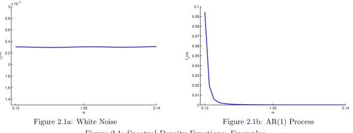
The spectral density function provides the information on the extent to which a specific frequency contributes to the variance of the series. To see this, we plot the spectral density of (1) white noise process (Figure 2.1a) and (2) AR (1) process (Figure2.1b). In particular, we set the standard deviation of the innovation terms in each series as0.038and the persistence termρas0.95for the AR (1) process.4 The horizontal axis denotes the frequency from low (0.13) to high (3.14) and the vertical axis denotes the spectral density corresponding to each frequency. Since the white noise process is i.i.d. across time, the contributions of variances at each frequency are equivalent in Figure 2.1a. However, for AR (1) process, the long-run frequency contributes more to the dynamics of the simulated series since it is generated to be very persistent over time.

0.13 1.55 3.14 1.4 1.6 1.8 2 2.2 2.4 2.6 2.8 3x 10 −4 fY ( ω ) ω

Figure2.1a: White Noise

0.13 1.55 3.14 0 0.01 0.02 0.03 0.04 0.05 0.06 0.07 0.08 0.09 0.1 fY ( ω ) ω

Figure2.1b: AR(1) Process Figure 2.1: Spectral Density Functions: Examples

One good property of the spectral density is that the sum of all spectral density is equal to the variance of the variable. Formally,

V(Yt|Ri) =

Z π

−π

SYt|Ri(ω)dω (2.3) whereRiis the policy regimeiunder which the time seriesYtis simulated andVdenotes variance. Hence, we can interpret spectral density at each frequency as the variance at each frequency.

Main objective of the (macroprudential) policies is to stabilize the economy. Put it differently, the

4

(7)

spectral density can be used to evaluate the effectiveness of the policies, particularly on the heterogeneous effects on the variance at different frequency. This is important since a policy that is intended to stabilize the economy at some specific frequencies - a macroprudential policy is designed to stabilize the economy at the relative low frequency - may have an adverse effect at the different frequency. This property is known as the “design limit” of policy. For instance, Brock, Durlauf, and Rondina (2008) considers an example that shows a policy to minimize overall variance of a variable can increase the variance of the series at the relatively short frequency. The finding that the welfare cost from different policies can vary across frequencies when the utility function is not time-separable (Otrok(2001b)) further raises the importance of our approach to study frequency-specific effects of macroprudential policies.

The steps to evaluate the effectiveness of different macroprudential policies can be described as follows. 1. Simulate the model economy with all exogenous shocks under different policy regimes.

2. Filter the simulated series followingBaxter and King(1999) to obtain filtered series whose frequency are between 2 years/cycle and 28 years/cycle. This is because either too high or too low frequencies are not main concerns of the policies.

3. Compute the spectral density of the filtered series, take the average across simulations, and compare the density functions from different policy regimes.

In particular, we will consider the effectiveness of macroprudential policies relative to the benchmark economy without any such policies. If the policy is effective at some frequency, the spectral density will become lower than that from the benchmark economy. If it has an adverse effect, the spectral density will be above that obtained from the benchmark economy. Therefore, if a policy is effective in stabilizing the economy as a whole, the spectral density of the key macro variables, such as output, loan, consumption, and inflation rate, will be below the corresponding spectral density from the benchmark economy, which will be studied in details in Section 5.2.

3 The Model

The model introduced in this section is not particularly new by itself, but includes key features of models with financial frictions. In particular, our model builds upon the model developed by Iacoviello (2014)5; we incorporate New-Keynesian feature to the original setup by Iacoviello (2014), similarly to Canova, Coutinho, Mendicino, Pappa, Punzi, and Supera(2015). Our strategy to keep the model to be consistent

5

(8)

with the previous literature is in order for minimizing the model-specific factors that can possibly affects the equilibrium behaviors.

The economy consists of patient households, impatient households, entrepreneurs, retail banks, invest-ment banks, retailers, and monetary authority. Two financial intermediaries have different roles in the economy; retail bank lends funds to both impatient household and investment bank where it uses deposits from patient household. Investment bank, however, obtains fund only from the retail bank and lends to entrepreneur. For the smoothing behavior of macro variables, habit formation and various adjustment costs are considered. Contrary toIacoviello(2014), we abstract from two non-financial shocks, preference shocks (that affect both of demand for consumption and housing) and investment-specific technology shocks since their roles are found to be small in his paper.

3.1 Households There is a measure one patient household (saver) and another measure one impatient

household (borrower). As usually assumed in the literature, patient households have a higher discount factor than impatient households, namely βs > βb > 0. Hence, in equilibrium only patient households

save while impatient households borrow.

3.1.1 Patient Households The representative patient households solve the following expected

life-time utility maximization problem by choosing optimal consumption C_ts, hours worked N_ts, housing H_ts, capital holding K_ts and saving in the bankDs_t, taking prices as given:

max E0 ∞ X t=0 β_st " ln C_ts−hC_ts₋₁ +εh_tν_hslnH_ts−ν_ns(N s t)1+φ 1 +φ # (3.1)

where βs ∈ (0,1) is the discount factor of patient households, h ∈ [0,1] is the parameter that governs

habit formation, φ >0is the inverse Frisch elasticity, andν_hs>0(resp. ν_ns >0) is the relative utility from housing (resp. working). εh

t is the exogenous shock to housing preference, which is one of the financial

shocks in our model economy.

Constraints for the patient households are as follows.

C_ts+K_ts+p_tHH_ts−H_ts−1 +dt+ACds_,t+AC_Ks_,t=w_tsN_ts+r_td₋₁d_t₋₁+ (r_tK+ 1−δ)K_ts₋₁ (3.2) ACd,t= ιd 2 (dt−dt−1)2 d (3.3) ACKs_,t = ιK s 2 K_ts−K_ts−1 2 Ks (3.4)

(9)

where the price of consumption goods is normalized to 1 (Pt ≡1), pHt is the real price of housing, rdt−1

is the gross real interest rate from the deposit, rK_t is the net rate of return from the physical capital, ws_t

is the real wage rate for patient households, ACd,t(resp. ACKs_,t) is the convex real external adjustment costs for deposit (resp. capital), ιHs, ι_Ks ≥0 are the parameters in the adjustment cost functions, andd (resp. Ks_{) is the steady state deposit (resp. capital holding) by patient households.}

3.1.2 Impatient Households The problem of the impatient households is similar to that of patient

households: max E0 ∞ X t=0 β_bt " ln C_tb−hC_tb−1 +εh_tν_hblnH_tb−ν_nb N b t 1+φ 1 +φ # (3.5) subject to C_tb+pH_t h H_tb−H_tb−1 i +r_tb−1lbt−1+AClb_,t=w_tbN_tb+lb_t+εb_t (3.6) AC_lb_,t= ι_lb 2 l_tb−lb_t−1 2 lb (3.7) lb_t ≤ρblbt−1+ (1−ρb) " γHb_t Et pH_t₊₁H_tb r_tb₊₁ −ε b t # (3.8) whereLb

t are bank loans,wtb is the real wage rate for impatient households, rtb−1 is the gross real interest

rate on loans,ρb ∈[0,1]allows for slow adjustment of bank loan over time6 andεbt≥0is the default shock,

which is another financial shock in our model; this can be interpreted as the wealth redistribution shock between borrower and lender since this shock increases the net wealth of impatient household (borrower) while it lowers the net wealth of retail bank (lender).7 _{Contrary to} _Iacoviello _{(2014), the default shock} also negatively affects the borrowing constraint of the impatient household in order to capture the idea that default also affects the willingness of banks to lend to borrowers.

Constraint (3.8) is the borrowing constraint whereγ_tHb is defined as follows.

γ_tHb=γHb₀ εlb_t (3.9)

Hence, γ₀Hb is the equity requirement or loan-to-value (henceforth LTV) ratio cap for the impatient

6

For the parameters to govern slow adjustment of loans, see Canova, Coutinho, Mendicino, Pappa, Punzi, and Supera

(2015).

7

(10)

household. εlb

t captures subjective lenders perceptions of the riskiness of the housing wealth, which will

be referred as LTV shock, the last financial shocks in our model. We finally note that changingγ₀Hb is one form of the macroprudential policies that we consider; if γHb

0 is set to be lower than before, it becomes

more difficult for the impatient households to borrow from the financial intermediary against the collateral (housing) she holds.

Other equations, variables, and parameters are defined similarly to patient households’ problem.

3.2 Entrepreneurs A continuum of firms, denoted as e, are also distributed on the unit interval;

e∈[0,1]. The firms are run by entrepreneurs, who buy investment goods from the competitive final goods market and produce intermediate goods using capital, housing, and labor. The intermediate goods market where the output of the entrepreneurs is sold is also assumed to be competitive. The entrepreneurs face borrowing constraints when making financing decisions, whose lifetime utility is given as follows:

maxE0 ∞ X t=0 β_etlog C_te−hC_te−1 (3.10)

whereβe< βs is assumed and Cte is the consumption of the entrepreneur.

The constraints that the entrepreneur faces are given as follows.

C_te+K_te+pH_t [H_te−H_te₋₁] +ws_tN_ts+w_tbN_tb+r_tKK_ts₋₁+r_tele_t₋₁+ACKe_,t+AC_le_,t =pX_t Xt+ (1−δ)Kte−1+lte+εet (3.11) Xt=εzt K_te₋₁ωk K_ts₋₁1−ωkα H_te₋₁ν (N_ts)ωnN_tb1−ω n(1−α−ν) (3.12) l_te≤ρelet−1+ (1−ρe) γ_tHeEt P_te₊₁H_te r_te₊₁ +γ Ke t Kte−γtN e(wstNts+wtbNtb)−εet (3.13) ACKe_,t = ιK e 2 K_te−K_te−1 2 Ke (3.14) ACle_,t = ιl e 2 le_t −le_t₋₁2 le (3.15)

wherepX_t is the price of the good produced by the entrepreneurs andre_t is the gross real interest rate on entrepreneur loans.

Equation (3.11) is the budget constraint of the representative entrepreneur. Equation (3.12) is the production function; the firm produces outputs using Cobb-Douglass technology where εz_t is a neutral productivity shock, which is one of the non-financial shock in our model, and inputs include housing,

(11)

(physical) capital, and labor. The real adjustment cost functions are defined similarly to those of house-holds.

Lastly, equation (3.13) is the borrowing constraint for the entrepreneur. Similarly to Aoki, Benigno, and Kiyotaki (2009),Neumeyer and Perri(2005), and Iacoviello(2014), we introduce the working capital assumption that entrepreneurs pay for some portion of wage bills in advance, i.e 0 < γN e

t ≤ 1, and γ_tHe, γKe_t <1 is assumed so that the financial intermediaries ask for collateral due to lack of expertise on production process. ρe ∈[0,1]is the adjustment parameter for slowly moving borrowing constraint. Again, γ_tHe≡γ₀Heεle_t so thatγ₀He is the policy variable controlled by the government, which is the LTV regulation on the entrepreneurs’ house holding. Further, γ_tKe ≡γ₀Keε_tle and γ_tN e ≡γ₀N eεle_t . Hence, γ₀He (γ₀Ke, γ₀N e) measures the degree of loans market tightness andεle_t is another LTV shock on the entrepreneur’s assets, which is another financial shock. The role of εe_t, the default shock on entrepreneur, is similar to that of impatient household.

3.3 Retail Banks Retail banks obtain funds from deposits by patient households and lend to

impa-tient households and investment banks. We assume βr < βs. The utility maximization problem of the

representative retail bank, r ∈[0,1], is given by

maxE0 ∞ X t=0 β_rtlog C_tr−hC_tr−1 (3.16)

subject to the following constraints:

C_tr+l_tb+li_t+r_td₋₁dt−1+ACd,t+ACli_,t+AC_lb_,t =d_t+r_ti₋₁li_t₋₁+rb_tl_tb₋₁−εb_t−εi_t (3.17) AC_li_,t = ι_li 2 li_t−li_t₋₁2 li (3.18) lb_t+li_t−dt−εbt−εit≥ρr(ltb−1+lit−1−dt−1−εbt−1−εit−1) + (1−ρr)[ηtblbt+ηtilit−εbt−εit] (3.19)

where other real adjustment costs are defined similarly to the corresponding agents, r_ti is the gross real interest rate on investment bank loans, and

η_tj =η₀j+ηj₁ lt/Yt l/Y −1 where j={b, i} (3.20)

Constraint (3.17) is the budget constraint for the retail bank and constraint (3.19) is a capital adequacy regulation constraint. The default shocks of impatient households (εb_t) and investment banks (εi_t) lowers

(12)

the net worth of the retail banks. η_tj is the capital-asset coefficient; if it is zero, the particular asset j is considered to be riskless. ηj₀ >0 is the minimum capital requirement for the retail bank specific to the loan j. Assuming ηj₁ > 0, the coefficient is positively related to the ratio between loan to GDP ratio at

t and that at the steady state. Hence, this feature, which is another form of the macroprudential policy considered in this model economy, captures one of the main ideas of Basel III regulatory system that capital requirements need to be countercyclical.

3.4 Investment Banks Investment banks obtain funds from the retail banks and lend to entrepreneurs.

We assumeβi < βs. The utility maximization problem of the representative retail bank,i∈[0,1], is given

by maxE0 ∞ X t=0 β_itlog C_ti−hC_ti−1 (3.21)

subject to the following constraints:

C_ti+le_t +r_ti−1lit−1+ACle_,t+AC_li_,t=l_ti+r_tel_te₋₁+εi_t−εe_t (3.22)

li_t≤ρilti−1+ (1−ρi)[(1−ηet)lte−εit−εet] (3.23)

where η_te is defined similarly toη_ti and η_tb and is the tool as a macroprudential policy. Constraint (3.22) is the budget constraint for the investment banks and the last constraint (3.23) is a borrowing constraint for the investment banks.

3.5 Retailers Monopolistic competitive retailers purchases goods from the entrepreneurs in a

compet-itive market and differentiates them into intermediate goods, as in the typical New Keynesian literature. The technology is linear: Yt(z) = Xte−F(z) where F(z) are fixed costs to make steady-state profit of

the retailer zero. Then retailers sell intermediate goods, Yt(z), to the final goods-producing firm at price Pt(z). Final output Yt is given by

Yt= Z 1 0 Yt(z) ε−1 ε dz _ε₋ε₁ (3.24) whereε >1.

(13)

Yt(z) = Pt(z) Pt −ε Yt (3.25)

and the aggregate price index

Pt= Z 1 0 Pt(z)1−εdz ₁−1ε (3.26)

Each retailer chooses optimal pricePt(z); followingCalvo(1983), the retailer can adjust the price with

probability 1−θ. If the retailer is not able to adjust its price,Pt(z) =Pt−1(z). Each retailer maximizes

its market value:

max Pt(z) E0 ∞ X t=0 β_stλs_t[Pt(z)Yt(z)−PteXte] (3.27)

subject to the equation (3.25). The optimal price level for firmz in periodt is:

P_t∗(z) = ε

ε−1

EtP∞j=0(θβs)jλst+jPtε+jYt+jPte+j

EtP∞_j₌₀(θβs)jλs_t₊_jP_tε₊_jYt+j

(3.28)

We assume a symmetric equilibrium case where P_t∗ = P_t∗(z),∀z, thus the aggregate price level evolves according to Pt= h (1−θ)(P_t∗)1−ε+θ(Pt−1)1−ε i₁₋1_ε (3.29)

3.6 Monetary Authority We assume that the monetary authority conducts a monetary policy

following the extended Taylor rule, which incorporate the loan (or credit)-to-GDP ratio as an additional determinant of the policy rate Ri_t, the nominal inter-bank interest rate:

Ri_t Ri = " _Ri t−1 Ri ρR Πt Π γΠ Yt Y γY lt l γL1−ρR# εR_t (3.30)

wherelt=lbt+lte+litand the target interest rate is the inter-bank interest rate,rti. It becomes a standard

(14)

3.7 Housing Market We assume that housing supply is exogenously given asH¯. Then the housing

market clearing condition is given by

¯

H=H_ts+H_tb+H_te (3.31) In what follows, we normalizeH¯ as one, without loss of generality.

3.8 Exogenous Shocks We have two non-financial shocks (TFP shock (εzt) and monetary policy

shock (εR_t )) and six financial shocks (three default shocks (εb_t, εe_t, andεi_t), two LTV shocks (εlb_t and εle_t ), housing preference shock (εh_t)) hence 8 exogenous shocks as total. Let εt denotes the exogenous shock

except the default shocks. It is assumed to follow AR (1) process:

logεt=ρlogεt−1+ut (3.32)

whereutis the i.i.d. shock that is normally distributed with mean 0 and variance σε. Default shocks are

defined as level instead of log level.

4 Calibration

4.1 Parameterization In calibrating parameters, we use the estimated values fromIacoviello(2014),

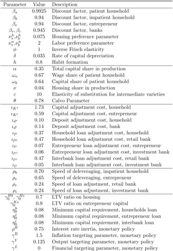
for the parameters that are common between our model and his model. If the parameter is not present in his paper, we use the parameter values that are commonly used in the literature. For instance, we set the patient household’s discount factor at 0.9925 to target the 3% annual risk-free interest rate. As in Iacoviello (2014), our value for capital depreciation is higher than the typical number in the literature, 0.025, because housing is additional factor of production which does not depreciate. Following standard NK-DSGE literature, the elasticity of substitution for intermediate varieties, ε, is calibrated as 10 to target the steady state mark-up is 10%. The coefficients in the Taylor rule are also the usual numbers to ensure the unique equilibrium of the model. Parameters related to macroprudential policies will be described later. Table 4.1 shows our benchmark calibration for the parameters and Table 4.2represents the parameterization for exogenous shocks used in our model.

4.2 Basic Results: Impulse Response Functions We will compare five model economies which

only differ in the macroprudential policies implemented. The benchmark economy (Model 1) is subject to 70% LTV ratio (γHb = 0.7), 8% constant minimum capital requirement, and monetary policy neutral

(15)

Table 4.1: Benchmark Calibration (Benchmark Economy) Parameter Value Description

βs 0.9925 Discount factor, patient household βb 0.94 Discount factor, impatient household βe 0.94 Discount factor, entrepreneur

βr, βi 0.945 Discount factor, banks

ν_sh,ν_bh 0.075 Housing preference parameter

ν_sn,ν_bn 2 Labor preference parameter

φ 1 Inverse Frisch elasticity

δ 0.035 Rate of capital depreciation

h 0.8 Habit formation

α 0.35 Total capital share in production

ωn 0.67 Wage share of patient household ωk 0.64 Capital share of patient household

ν 0.04 Housing share in production

ε 10 Elasticity of substitution for intermediate varieties

θ 0.78 Calvo Parameter

ιKs 1.73 Capital adjustment cost, household

ιKe 0.59 Capital adjustment cost, entrepreneur

ιds 0.10 Deposit adjustment cost, household

ιdr 0.14 Deposit adjustment cost, bank

ι_lb 0.37 Household loan adjustment cost, household

ι_lbr 0.47 Household loan adjustment cost, retail bank

ιle 0.07 Entrepreneur loan adjustment cost, entrepreneur

ι_lei 0.06 Entrepreneur loan adjustment cost, investment bank

ι_lir 0.47 Interbank loan adjustment cost, retail bank

ι_li 0.05 Interbank loan adjustment cost, investment bank

ρb 0.70 Speed of deleveraging, impatient household ρe 0.65 Speed of deleveraging, entrepreneur

ρr 0.24 Speed of loan adjustment, retail bank ρi 0.24 Speed of loan adjustment, investment bank γ₀Hb,γ₀He 0.7 LTV ratio on housing

γ₀Ke 0.9 LTV ratio on entrepreneur capital

η₀b 0.08 Minimum capital requirement, households loan

η₀e 0.08 Minimum capital requirement, entrepreneur loan

η₀i 0.08 Minimum capital requirement, interbank loan

ρR 0.75 Interest rate inertia, monetary policy

γΠ 1.5 Inflation targeting parameter, monetary policy

γY 0.125 Output targeting parameter, monetary policy

γL 0 Financial targeting parameter, monetary policy

to loan changes. Other economies have different policy measures as follows:

(16)

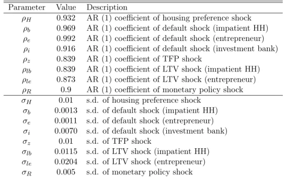
Table 4.2: Benchmark Calibration: Exogenous Shocks Parameter Value Description

ρH 0.932 AR (1) coefficient of housing preference shock ρb 0.969 AR (1) coefficient of default shock (impatient HH) ρe 0.992 AR (1) coefficient of default shock (entrepreneur) ρi 0.916 AR (1) coefficient of default shock (investment bank) ρz 0.839 AR (1) coefficient of TFP shock

ρlb 0.839 AR (1) coefficient of LTV shock (impatient HH) ρle 0.873 AR (1) coefficient of LTV shock (entrepreneur) ρR 0.9 AR (1) coefficient of monetary policy shock σH 0.01 s.d. of housing preference shock

σb 0.0013 s.d. of default shock (impatient HH) σe 0.0011 s.d. of default shock (entrepreneur) σi 0.0070 s.d. of default shock (investment bank) σz 0.01 s.d. of TFP shock

σlb 0.0115 s.d. of LTV shock (impatient HH) σle 0.0204 s.d. of LTV shock (entrepreneur) σR 0.005 s.d. of monetary policy shock

• Model 2: Extended Taylor rule (γL= 0.125)

• Model 3: Countercyclical capital requirement (η_j1= 0.15 for j=b, i, e)

• Model 4: Tightening LTV ratio on impatient household (γ₀Hb= 0.5)

• Model 5: All three policies (γL= 0.125,η_j1= 0.15 for j=b, i, e,γHb₀ = 0.5)

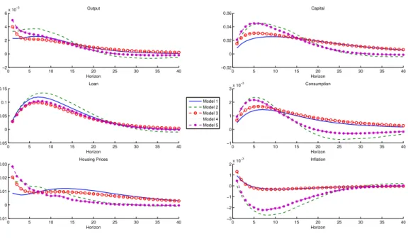
Before we present our main results, we first show the impulse response functions to some exogenous shocks (TFP shock, LTV shock (on entrepreneur), default shock (on entrepreneur), and housing preference shock) of our model economy to check if the model behaves well consistently with the usual economic intuition and to check if different policies result in different impulse responses of the variables.

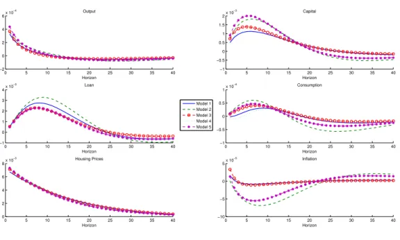
4.2.1 Comparing Effects of Different Policies with IRFs Figure 4.2.1 is the collection of

impulse response functions to one-time-one-unit shock to aggregate productivity. As usually argued in the literature, different sets of macroprudential policies do not have much impact on responses of macro variables when the real shock hits the economy. Figure4.2is the collection of impulse response functions to one-time-one-unit shock to LTV on entrepreneurs. Since positive shock on LTV of entrepreneurs means that they can borrow more given the same asset values, this shock stimulates the economy. Overall, different macroprudential policies are still not effective to lower responsiveness of the economy to the

(17)

shock. Figure 4.3 plots impulse response functions to the positive shock to default of entrepreneurs; as this is a negative redistribution shock for the banks, they will lower loans, which triggers economic downturns. While some macroprudential policies (countercyclical capital requirement in particular) seem to be effective in lowering output and loan fluctuations, most other policies are not effective. Lastly, Figure 4.4 presents impulse response functions to a shock to housing preference of households. Given fixed housing supply, more housing demand means that the housing price increases, which increases the wealth of average agents in this economy. Hence, the economy experiences boom. Note, again, the macroprudential policies are not effective in terms of lowering responsiveness of the economy.

Therefore, a quick preview of the effectiveness of different policies with impulse response functions shows that in most cases macroprudential policies do not achieve their goals to lower the effects of ex-ogenous shocks. If any, it is mostly observed from the policy that requires the banks to accumulate countercyclical capital buffers.

0 5 10 15 20 25 30 35 40 0 0.5 1 1.5 2 2.5x 10 −3 Horizon Consumption 0 5 10 15 20 25 30 35 40 0 0.005 0.01 0.015 0.02 0.025 Horizon Capital 0 5 10 15 20 25 30 35 40 −0.01 0 0.01 0.02 0.03 Horizon Loan Model 1 Model 2 Model 3 Model 4 Model 5 0 5 10 15 20 25 30 35 40 0 0.002 0.004 0.006 0.008 0.01 Horizon Output 0 5 10 15 20 25 30 35 40 0 0.005 0.01 0.015 0.02 Horizon Housing Prices 0 5 10 15 20 25 30 35 40 −8 −6 −4 −2 0x 10 −4 Horizon Inflation

Figure 4.1: Impulse Response Functions: Productivity Shock

Note: Model 1 is the benchmark economy, Model 2 is the economy with extended Taylor rule, Model 3 is the economy with countercyclical capital requirement policy, Model 4 is the economy with tight LTV on impatient household, and Model 5 is the economy with all macroprudential policy.

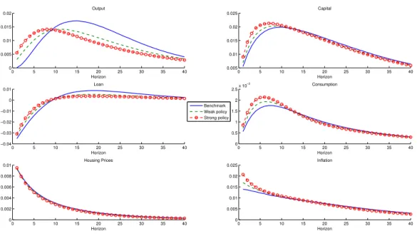
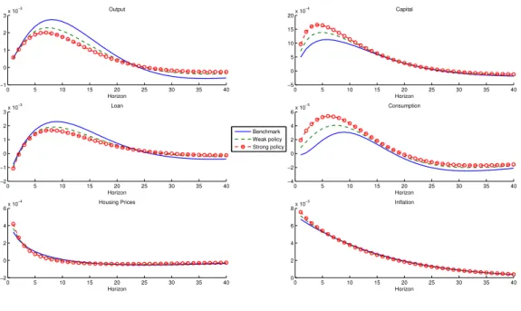
4.2.2 Effectiveness of More Aggressive Policy In this section, we evaluate the performance

of more aggressive macroprudential policy. In particular, we consider the macroprudential policy on countercyclical capital requirement, since it seems to be more effective than other policies. Figure 4.5

(18)

0 5 10 15 20 25 30 35 40 −1 0 1 2 3x 10 −3 Horizon Consumption 0 5 10 15 20 25 30 35 40 −0.02 0 0.02 0.04 0.06 Horizon Capital 0 5 10 15 20 25 30 35 40 −0.05 0 0.05 0.1 0.15 Horizon Loan 0 5 10 15 20 25 30 35 40 −2 0 2 4 6x 10 −3 Horizon Output Model 1 Model 2 Model 3 Model 4 Model 5 0 5 10 15 20 25 30 35 40 −0.01 0 0.01 0.02 0.03 Horizon Housing Prices 0 5 10 15 20 25 30 35 40 −3 −2 −1 0 1 2x 10 −3 Horizon Inflation

Figure 4.2: Impulse Response Functions: LTV Shock to Entrepreneur

0 5 10 15 20 25 30 35 40 −3 −2 −1 0 1x 10 −4 Horizon Consumption 0 5 10 15 20 25 30 35 40 −5 −4 −3 −2 −1 0x 10 −3 Horizon Capital 0 5 10 15 20 25 30 35 40 −0.015 −0.01 −0.005 0 Horizon Loan Model 1 Model 2 Model 3 Model 4 Model 5 0 5 10 15 20 25 30 35 40 −6 −5 −4 −3 −2 −1 0x 10 −4 Horizon Output 0 5 10 15 20 25 30 35 40 −20 −15 −10 −5 0 5x 10 −4 Horizon Housing Prices 0 5 10 15 20 25 30 35 40 −2 −1 0 1 2 3 4x 10 −4 Horizon Inflation

Figure 4.3: Impulse Response Functions: Default Shock to Entrepreneur

(19)

0 5 10 15 20 25 30 35 40 −1 −0.5 0 0.5 1x 10 −4 Horizon Consumption 0 5 10 15 20 25 30 35 40 −1 −0.5 0 0.5 1 1.5 2x 10 −3 Horizon Capital 0 5 10 15 20 25 30 35 40 −1 0 1 2 3 4x 10 −3 Horizon Loan 0 5 10 15 20 25 30 35 40 −2 0 2 4 6x 10 −4 Horizon Output Model 1 Model 2 Model 3 Model 4 Model 5 0 5 10 15 20 25 30 35 40 0 2 4 6 8x 10 −3 Horizon Housing Prices 0 5 10 15 20 25 30 35 40 −10 −5 0 5x 10 −5 Horizon Inflation

Figure 4.4: Impulse Response Functions: Housing Preference Shock

to 4.7 show the impulse response functions to productivity shock, default shock to entrepreneurs, and housing preference shock, respectively. The thick blue line represents the responses from the benchmark economy, the dotted green line represents the economy with weak macroprudential policy (η1_j = 0.15 for

j =b, i, e), and the circled red line represents the economy with strong macroprudential policy (η_j1= 0.30

for j=b, i, ehence the coefficient is twice from the weak policy economy).

We first note that in terms of lowering loan responses, the strong macroprudential policy is mostly effective. i.e. the strong policy achieves its goal to stabilize financial market more effectively than the weak policy does. Furthermore, when the economy experiences a recession due to the default shock to entrepreneur, the strong macroprudential policy is particularly effective in lowering output and loan fluctuations. If other shocks hits the economy, the responses of variables are heterogeneous across different policy regimes so that we cannot easily determine the overall effectiveness of macroprudential policies.

5 Frequency-Specific Effects from the Model Economy

5.1 Volatility at Business Cycle Frequency Before we proceed to analyze the frequency-specific

(20)

0 5 10 15 20 25 30 35 40 0 0.5 1 1.5 2 2.5x 10 −3 Horizon Consumption 0 5 10 15 20 25 30 35 40 0.005 0.01 0.015 0.02 0.025 Horizon Capital 0 5 10 15 20 25 30 35 40 −0.04 −0.03 −0.02 −0.01 0 0.01 Horizon Loan 0 5 10 15 20 25 30 35 40 0 0.005 0.01 0.015 0.02 Horizon Output Benchmark Weak policy Strong policy 0 5 10 15 20 25 30 35 40 0 0.002 0.004 0.006 0.008 0.01 Horizon Housing Prices 0 5 10 15 20 25 30 35 40 0 0.005 0.01 0.015 0.02 0.025 Horizon Inflation

Figure 4.5: Impulse Response Functions: Productivity Shock

Note: ‘Benchmark’ denotes the economy withη1j= 0, ‘Weak policy’ is the economy with countercyclical capital requirement policy withη1

j = 0.15, and ‘Strong policy’ is the economy with countercyclical capital requirement policy withηj1= 0.3for

j=b, i, e. 0 5 10 15 20 25 30 35 40 −1.5 −1 −0.5 0x 10 −4 Horizon Consumption 0 5 10 15 20 25 30 35 40 −3 −2.5 −2 −1.5 −1 −0.5x 10 −3 Horizon Capital 0 5 10 15 20 25 30 35 40 −10 −5 0 5x 10 −3 Horizon Loan Benchmark Weak policy Strong policy 0 5 10 15 20 25 30 35 40 −0.015 −0.01 −0.005 0 Horizon Output 0 5 10 15 20 25 30 35 40 −6 −5 −4 −3 −2 −1 0x 10 −4 Horizon Housing Prices 0 5 10 15 20 25 30 35 40 −20 −15 −10 −5 0 5x 10 −4 Horizon Inflation

Figure 4.6: Impulse Response Functions: Default Shock to Entrepreneur

(21)

0 5 10 15 20 25 30 35 40 −4 −2 0 2 4 6x 10 −5 Horizon Consumption 0 5 10 15 20 25 30 35 40 −5 0 5 10 15 20x 10 −4 Horizon Capital 0 5 10 15 20 25 30 35 40 −2 −1 0 1 2 3x 10 −3 Horizon Loan Benchmark Weak policy Strong policy 0 5 10 15 20 25 30 35 40 −1 0 1 2 3x 10 −3 Horizon Output 0 5 10 15 20 25 30 35 40 −2 0 2 4 6x 10 −4 Horizon Housing Prices 0 5 10 15 20 25 30 35 40 0 2 4 6 8x 10 −3 Horizon Inflation

Figure 4.7: Impulse Response Functions: Housing Preference Shock

j=b, i, e.

cycle frequency. In particular, we simulated the model economy 1,000 times with each simulation has total period as 1,024. We then filter each of the series with κ = 200 by applying the band-pass filter (Baxter and King (1999)) to obtain series of frequency between 2 years/cycle and 8 years/cycle where

κ is the number of leads/lags used in the approximation of the filtering (see Otrok (2001b) for choosing

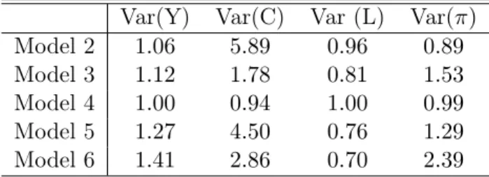
T = 1,024 and κ = 200). We then compute the variance of each series8, and take the average of the variances from each simulation. Table 5.1summarizes the results.

Several observations are noteworthy. First, economic fluctuations in the real sector are overall amplified under any of the macroprudential policies while loan fluctuations are overall stabilized. While the extended Taylor rule (Model 2) amplifies the variance of consumption compared to that from the benchmark economy more than other policies, it is more successful in achieving (in relative terms) stabilizing other variables. For instance, the variance of output all increase except the model 4 with tightened LTV ratio but the increase is the smallest in Model 2. In addition, the variance of inflation rate, Var(π), which is one of the main variables of interest by the central bank, is minimized under the extended Taylor rule. Hence, depending on the form of the loss function, which is a function of output volatility and inflation volatility, the extended Taylor rule can provide higher social welfare than other policies and no policy

8_{Here we use the variance since the spectral density provides variance at each frequency. Information contained in the}

(22)

Table 5.1: Relative Variance of Key Variables Var(Y) Var(C) Var (L) Var(π) Model 2 1.06 5.89 0.96 0.89 Model 3 1.12 1.78 0.81 1.53 Model 4 1.00 0.94 1.00 0.99 Model 5 1.27 4.50 0.76 1.29 Model 6 1.41 2.86 0.70 2.39

Note: All values are relative to the benchmark economy. Model 2 is the economy with extended Taylor rule, Model 3 is the economy with countercyclical capital requirement policy, Model 4 is the economy with tight LTV on impatient household, and Model 5 is the economy with all macroprudential policy. Model 6 is the economy with strong countercyclical capital requirement policy.

economy. Second, stabilizing the financial market at the business cycle frequency is the most successful in economies with countercyclical capital requirement policy (Model 3 (weak policy) and Model 6 (strong policy)). Third, the macroprudential policy that particularly affects LTV ratio of impatient households (model 4) is not overall effective. Finally, the strong macroprudential policy (Model 6) is more effective in the financial market than the weak policy (Model 3) but at the cost of amplifying the fluctuation in the real sector more.

Overall, two policies, extended Taylor rule and countercyclical capital requirement policy, seem to be relatively effective at the business cycle frequency from Table 5.1. In the next section, we will study if this conclusion is still preserved if we compute the variance at different frequencies.

5.2 Frequency-Specific Effects of Different Policies We now turn to our main analysis,

which analyzes the frequency-specific effects of macroprudential policies. In so doing, we take the steps described in Section 2. Again, numbers of simulation are1,000and total period of each simulation is set to be 1,024. When filtering the series, we setκ= 200when applying the band-pass filter to obtain series of frequency between 2 years/cycle and 28 years/cycle where κ is the number of leads/lags used in the approximation of the filtering. The results we report in this section still survive even when we use the original data without filtering.

Since our main purpose here is to evaluate the performance of different policies relative to the bench-mark economy without considering any macroprudential policy, we compute the spectral density of each variable under the specific policy regime relative to that under the benchmark model. We particularly consider four macro variables in this exercise; output, loan, consumption, and inflation rate. Figure 5.1

to 5.4show the results. In each figure, the vertical axis denotes the spectral density relative to model 1 at each frequency and the horizontal axis denotes frequencies from low to high frequency.

(23)

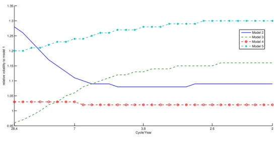
Firstly, contrary to the usual expectation that output fluctuations will be stabilized under the policy, the volatility is amplified almost at every frequency regardless of different policy. The only exception is the countercylical capital requirement policy (Model 3); it lowers the spectral density at the very low frequency (lower than 12 years/cycle) so that the policy is effective at the relative low frequency. However, at the higher frequency, the volatility becomes larger than that in the benchmark economy. i.e. there is a design limit in this particular policy at the high frequency; at the cost of increasing output fluctuations at the high frequency (higher than 12 years/cycle), it can stabilize the economy at the low frequency. Other policies do not, unfortunately, stabilize the economy at all. For instance, the extended Taylor rule, which is designed to fight against the loan stabilization, amplifies the volatility at each frequency by more than 10% than the economy without any policy. The amplification of fluctuations in the real sector is also observed in Figure 5.2; except the policy to tighten LTV ratio on impatient household (Model 3), consumption volatility is exacerbated under any policies. Especially the extended Taylor rule amplifies the consumption fluctuations by about 6.5 times from the benchmark ones. In summary, the macroprudential policies considered in our model economy are not overall effective in stabilizing the real sector of the economy. 28.4 7 3.8 2.6 2 0.95 1 1.05 1.1 1.15 1.2 1.25 1.3 1.35 Cycle/Year

relative volatility to model 1

Model 2 Model 3 Model 4 Model 5

Figure 5.1: Frequency-Specific Effects: Output

Note: Relative volatility compared to model 1 at each frequency; Model 2 is the economy with extended Taylor rule, Model 3 is the economy with countercyclical capital requirement policy, Model 4 is the economy with tight LTV on impatient household, and Model 5 is the economy with all macroprudential policy.

How about the loan fluctuations, which is the main objective of macroprudential policy? Figure 5.3

shows the result, which satisfies its main goal. Almost every policies are effective in stabilizing the financial market, in terms of loan fluctuations. For instance, the countercyclical capital requirement policy (Model

(24)

28.40 7 3.8 2.6 2 1 2 3 4 5 6 7 8 Cycle/Year

Figure 5.2: Frequency-Specific Effects: Consumption

3) is very effective since it lowers the loan volatility by about 20% at every frequency than the baseline economy. While the extended Taylor rule (Model 2) is not effective at the relatively low frequency, it becomes effective in stabilizing the financial market at near 10 years/cycle. In the mean time, the policy to tighten LTV ratio on impatient household (Model 4) is not that effective in the financial market as well as in the goods market. This means that to tighten LTV ratio of impatient households is not overall effective in any markets in our model economy. The economy which implements all of the above policies (Model 5) is also effective in stabilizing the financial market.

We first point out that tightening LTV ratio is not overall effective since it is not the policy that reacts to the changes in the economy; other policies, in contrast, react to the changes in the aggregate variables such as the loan to GDP ratio. Rather, LTV policy only changes the steady-state of the economy but not react to the fundamental changes so that it is not effective. In contrast, the countercyclical capital requirement policy is effective since it really reacts to the fluctuations in loan to GDP ratio. It is effective in lowering loan fluctuation at every frequency since banks accumulates enough capital during boom for possible losses during recessions, which results in less changes in overall loan level. In contrast, it can have a negative effect on GDP in the following sense; given loan size at the beginning of the period, lower output due to some exogenous shocks increases loan to output ratio so that banks accumulate more capital during the recessionary periods, which can potentially amplify rather than lower output fluctuations.

(25)

Policies are again not that effective in lowering the variance of inflation rate at different frequencies. Rather, the negative effect of the countercyclical capital requirement policy (Model 3) on the fluctuations of inflation rate is amplified at the higher frequency. One interesting finding is that the policy rules that directly changes the Taylor rule (Model 2 and Model 5) are effective in lowering the spectral density of inflation rate at the relatively high frequency while they have very large negative effects at the low frequency. Specifically, the effectiveness of the policy increases as frequency becomes higher. This is because the Taylor rule itself is designed to or found to be effective in lowering inflation fluctuations at the business cycle frequency. As a result, as soon as the lower frequency is considered in the analysis, its effectiveness may disappear. Hence, our result provides a lesson for the central bank; if the central bank really cares about the inflation rate (as all central banks do), it may not be a good idea to extend the Taylor rule such a way to respond to loan fluctuations.

In summary, our exercise implies that the currently well-known macroprudential policies are effective in stabilizing the financial market, as is designated. However, there is a substantial cost to achieve its effectiveness in the financial sector; it amplifies the fluctuations in the real sector. Especially the performance of the extended Taylor rule is worse than other policies in many dimensions while that of countercyclical capital requirement policy is effective even in the goods market at the very low frequency. Contrary to these policies, tightening LTV ratio on impatient households does not affect the economy much compared to other policies. Hence, the design limit of macroprudential policy in our model is two folds. First, the financial sector stabilization is associated with the real sector destabilization. Second, the effectiveness of policy is different across frequencies; for instance, the relative output variance increases as frequency becomes higher when the countercyclical capital requirement policy is implemented while the opposite is observed with the extended Taylor rule.

We finally note that our conclusion from the analysis with filtered data at business cycle frequency on the effectiveness of the extended Taylor rule is now overturned. In the previous section we showed with Table 5.1 that the extended Taylor rule performs relatively well compared to other policies. This does not hold, however, in the frequency-specific analysis since the former analysis only considered the effects of the policies at the business cycle frequency (2-8 years). This comes from the fact that the variances of output (Figure 5.1) and that of inflation rate (Figure 5.4) are much greater at the relatively low frequency (longer than 7 years) when the policymaker implements the extended Taylor rule. Since the macroprudential policy is designed to stabilize the financial cycles, which is believed to exhibit much lower frequency than the business cycle frequency, this implies that the bad performance of the extended Taylor rule is hidden under the usual analysis that computes the variance (standard deviation) of the

(26)

macro variables filtered to exhibit 2-8 years of cycles. 28.4 7 3.8 2.6 2 0.7 0.8 0.9 1 1.1 1.2 1.3 1.4 Cycle/Year

Figure 5.3: Frequency-Specific Effects: Loan

28.40 7 3.8 2.6 2 1 2 3 4 5 6 7 8 9 Cycle/Year

Figure 5.4: Frequency-Specific Effects: Inflation

Next, we study if the effects of strict macroprudential policy can be different from the less strict macro-prudential policy. As in the previous section, we only consider the countercyclical capital requirement policy since it is the most effective policy in terms of loan market stabilization. We again compute the

(27)

relative spectral density of the economy with weak macroprudential policy (η1

j = 0.15 forj =b, i, e, thick

blue line) and the economy with strong macroprudential policy (η_j1 = 0.30 for j = b, i, e, circled green line) and plot the spectral densities in Figure 5.5.

Two conclusions can be drawn from the figures. First, the strong policy is more effective in stabilizing the financial market than the weak one, as is expected. This achievement, however, is associated with the costs of amplifying the fluctuations in the real sector than the weak policy. Particularly, the output, consumption, and inflation rate volatility at each frequency are much more exacerbated under the strong policy. Even worse, the negative effects in the real sector increase in the frequency. If the monetary authority cares about the aggregate fluctuations at the business cycle frequency, which is usually defined as the fluctuations between about 2 years/cycle and 8 years/cycle, the strong macroprudential policy is not recommended; it increases output volatility compared to the benchmark economy about 40%, consumption volatility about 200%, and inflation rate volatility more than 100% at the business cycle frequency. 28.4 7 3.8 2.6 2 0.9 1 1.1 1.2 1.3 1.4 1.5 1.6 Cycle/Year

Output 28.4 7 3.8 2.6 2 0.5 0.6 0.7 0.8 0.9 Cycle/Year Loan 28.41 7 3.8 2.6 2 1.5 2 2.5 3 3.5 Cycle/Year Consumption Weak Policy Strong Policy 28.41 7 3.8 2.6 2 1.5 2 2.5 Cycle/Year Inflation

Figure 5.5: Frequency-Specific Effects: Weak vs. Strong Policy

Note: Relative volatility compared to model 1 at each frequency. ‘Weak policy’ is the economy with countercyclical capital requirement policy withη1j= 0.15, and ‘Strong policy’ is the economy with countercyclical capital requirement policy with

η1

(28)

6 Conclusion

We evaluate the performances of various macroprudential policies in this paper, within an extended New Keynesian model. Our results from the conventional macroprudential policy are somewhat negative. They can achieve their goals to stabilize the financial market while they can amplify the volatility in the real sector. Our findings further indicate that effectiveness of most macroprudential policies can vary across frequencies but above conclusion is not overturned whether we study the frequency-specific effects or not. However, the extended Taylor rule has clear frequency-specific effects so that it should be carefully evaluated using our approach.

One possibility to understand our results is that the policies are not “optimally” designed; they are originally intended to stabilize financial markets, hence there is an “unexpected” cost associated with such a policy, as shown in our paper. Therefore, the future research needs to find the optimally designed macroprudential policy so that it can achieve its main goal while the adverse effect is minimized. Other possibility is that the model we consider in this paper is not able to fully capture the positive effects from such policies on the real sector. In this regard, studies with alternative models will be another direction in evaluating the performances of macroprudential policy.

(29)

References

Angeloni, I., and E. Faia (2013): “Capital Regulation and Monetary Policy with Fragile Banks,” Journal of Monetary Economics, 60(3), 311–324. 1

Aoki, K., G. Benigno, and N. Kiyotaki (2009): “Capital Flows and Asset Prices,” in NBER In-ternational Seminar on Macroeconomics 2007, ed. by R. Clarida, and F. Giavazzi, pp. 175–216. The University of Chicago Press. 10

Bailliu, J., C. Meh, andY. Zhang(2015): “Macroprudential rules and monetary policy when financial frictions matter,” Economic Modelling, 50, 148–161. 1

Baxter, M., andR. G. King(1999): “Measuring Business Cycles: Approximate Band-Pass Filters For Economic Time Series,” Review of Economics and Statistics, 81(4), 575–593. 6,20

Benes, J., and M. Kumhof (2015): “Risky bank lending and countercyclical capital buffers,” Journal of Economic Dynamics and Control, 58, 58–80. 1

BIS (2010): “Macroprudential Instruments and Frameworks : A Stocktaking of Issues and Experiences,” Committee on the Global Financial System. 1,3

Borio, C.(2012): “The financial cycle and macroeconomics: What have we learnt?,” BIS Working Papers No. 395. 1

Brock, W. A., S. N. Durlauf, and G. Rondina (2008): “Frequency-Specific Effects of Monetary Policy Rules,” American Economic Review Papers and Proceedings, 98(2), 241–245. 2,4,6

(2013): “Design Limits and Dynamic Policy Analysis,” Journal of Economic Dynamics and Control, 37(12), 1421–1436. 2

Calvo, G. A. (1983): “Staggered Prices in a Utility-Maximizing Framework,” Journal of Monetary Economics, 12, 383–398. 12

Canova, F., L. Coutinho, C. Mendicino, E. Pappa, M. T. Punzi, and D. Supera(2015): “The Domestic and the International EÂćÂťects of Financial Disturbances,” Working Paper. 2,6,8

Collard, F., H. Dellas, B. Diba,andO. Loisel(2014): “Optimal Monetary and Prudential Policies,” Working Paper. 1

(30)

Hamilton, J. D. (1994): Time Series Analysis. Princeton University Press. 4

Iacoviello, M. (2005): “House Prices, Collateral Constraints and Monetary Policy in the Business Cycle,” American Economic Review, 95(3), 739–764. 6

(2014): “Financial Business Cycles,” Review of Economic Dynamics, Forthcoming. 2,6,7,8,10,

13

Kiley, M. T., and J. W. Sim (2014): “Optimal Monetary and Macroprudnetial Policies: Gains and Pitfalls in a Model of Financial Intermediation,” Working Paper. 2

Neumeyer, P. A., and F. Perri(2005): “Usiness Cycles in Emerging Economies: the Role of Interest Rates,” Journal of Monetary Economics, 52(2), 345–380. 10

Nguyen, T. T. (2014): “Bank Capital Requirements : A Quantitative Analysis,” Working Paper. 1 Otrok, C. (2001a): “On Measuring the Welfare Cost of Business Cycles,” Journal of Monetary

Eco-nomics, 47, 61–92. 3

(2001b): “Spectral Welfare Cost Functions,” International Economic Review, 42(2), 345–367. 6,

20

Quint, D., and P. Rabanal (2014): “Monetary and Macroprudential Policy in an Estimated DSGE Model of the Euro Area,” International Journal of Central Banking. 1

Schmitt-Grohé, S., andM. Uribe (2006): “Optimal Simple and Implementable Monetary and Fiscal Rules: Expanded Version,” NBER Working Paper No. 12402. 1

Suh, H. (2012): “Macroprudential Policy: Its Effects and Relationship to Monetary Policy,” Federal Reserve Bank of Philadelphia Working Paper No.12-28. 1

Van Den Heuvel, S. J. (2008): “The welfare cost of bank capital requirements,” Journal of Monetary Economics, 55(2), 298–320. 1

Woodford, M. (2012): “Inflation Targeting and Financial Stability,” Sveriges Riksbank Economic Re-view, 1. 2

(31)

A Equilibrium Conditions

A.1 Patient Household λst the Lagrangian multiplier attached to the budget constraint.

[C_ts] λs_t = 1 C_ts−hC_ts₋₁ −βsEt h C_ts₊₁−hC_ts (A.1) [K_ts] 1 +dACKs,t dK_ts =βsEt λs_t₊₁ λs_t (1 +r K t+1−δ) (A.2) [H_ts] pH_t = ε h tνhs H_tsλs_t +βsEt λs_t₊₁ λs_t p H t+1 (A.3) [N_ts] ws_t = ν s n(Nts)φ λs_t (A.4) [ds_t] 1 +dACd,t ddt =βsEt λs_t₊₁ λs_t r d t (A.5) [λs_t] C_ts+K_ts+pH_t H_ts−H_ts−1 +dt+ACds_,t+AC_Ks_,t=ws_tN_ts+r_td₋₁d_t₋₁+ (r_tK+ 1−δ)K_ts₋₁ (A.6)

A.2 Impatient Household λbt(resp. µbt) the Lagrangian multiplier attached to the budget constraint

(resp. borrowing constraint).

[C_tb] λb_t = 1 C_tb−hC_tb₋₁ −βbEt h C_tb₊₁−hC_tb (A.7) [H_tb] pH_t = ε h tνhb H_tbλb_t +βbEt " λb_t₊₁ λb_t p H t+1 # +µb_t(1−ρb)γtb pH_t₊₁ r_tb₊₁ (A.8) [N_tb] wb_t = ν b n(Ntb)φ λb t (A.9) [lb_t] 1−µb_t− dAClb,t dlb_t =βbEt " λb t+1 λb_t (r b t−ρbµbt+1) # (A.10) [λs_t] C_tb+pH_t hH_tb−H_tb₋₁i+rb_t₋₁l_tb₋₁+AC_lb_,t =wb_tN_tb+l_tb+εb_t (A.11) [µb_t] l_tb=ρbltb−1+ (1−ρb)γtHbEt pH_t₊₁H_tb rb t −εb_t (A.12)

A.3 Entrepreneur λet (resp. µet) the Lagrangian multiplier attached to the budget constraint (resp.

(32)

[C_te] λe_t = 1 C_te−hC_te₋₁ −βeEt h C_te₊₁−hC_te (A.13) [H_te] pH_t =βeEt λe_t₊₁ λe t pH_t₊₁(1 +r_tH₊₁) +µe_t(1−ρe)γtHe pH_t₊₁ re t+1 (A.14) [K_te] 1 +dACKe,t dK_te =βeEt λe_t₊₁ λe_t (1 +r K t+1−δ) +µe_t(1−ρe)γtKe (A.15) [N_ts] (1 + (1−ρe)γtN e)wstNts= (1−α−ν)ωnpXt Xt (A.16) [N_tb] (1 + (1−ρe)γtN e)wbtNtb = (1−α−ν)(1−ωn)pXt Xt (A.17) [r_tK] rK_t =α(1−ωk)pX_t Xt/Kts−1 (A.18) [l_te] 1 +dACle,t dl_te =µ e t+βeEt _λe t+1 λe_t (r e t+1−ρeµet+1) (A.19) [λe_t] C_te+K_te+pH_t [H_te−H_te₋₁] +ws_tN_ts+w_tbN_tb+r_tKK_ts₋₁+re_tle_t₋₁+ACKe_,t+AC_le_,t =pX_t Xt+ (1−δ)Kte−1+let+εet (A.20) [µe_t] le_t =ρelte−1+ (1−ρe) γ_tHeEt P_te₊₁H_te re t+1 +γ_tKeK_te−γ_tN e(w_tsN_ts+wb_tN_tb)−εe_t (A.21) where Xt =εzt Kte−1 αωk K_ts₋₁α(1−ωk) H_te₋₁ν(N_ts)(1−α−ν)ωn N_tb(1−α−ν)(1−ω n₎

. From the firm’s pro-duction function,pH

t rtH =νpXt Xt/Hte−1

A.4 Retail Banks λrt (resp. µrt) the Lagrangian multiplier attached to the budget constraint (resp.

(33)

[C_tr] λr_t = 1 C_tr−hC_tr₋₁ −βrEt h C_tr₊₁−hC_tr (A.22) [dt] 1− dACdr_,t ddt =µr_t +βrEt _λr t+1 λr_t (r d t −ρrµrt+1) (A.23) [lb_t] 1 +dAClbr,t dlb t =µr_t(1−(1−ρr)ηbt) +βrEt _λr t+1 λr t (rb_t−ρrµrt+1) (A.24) [l_ti] 1 +dAClir,t dli_t =µ r t(1−(1−ρr)ηit) +βrEt _λr t+1 λr_t (r i t−ρrµrt+1) (A.25) [λr_t] C_tr+lb_t+li_t+rd_t−1dt−1+ACd,t+ACli_,t+AC_lb_,t=d_t+ri_t₋₁l_ti₋₁+r_tblb_t₋₁−εb_t−εi_t (A.26) [µr_t] lb_t+l_ti−dt−εbt−εit=ρr(lbt−1+lti−1−dt−1−εbt−1−εit−1) + (1−ρr)[ηtblbt+ηitlti−εbt−εit] (A.27) (A.28)

A.5 Investment Banks λit (resp. µit) the Lagrangian multiplier attached to the budget constraint

(resp. borrowing constraint).

[C_ti] λi_t= 1 C_ti−hC_ti₋₁ −βiEt h C_ti₊₁−hC_ti (A.29) [le_t] 1 +dAClei,t dle_t =µ i t(1−ρi)(1−ηte) +βiEt _λi t+1 λi t re_t₊₁ (A.30) [l_ti] 1 +dACli,t dl_ti =µ i t+βiEt _λi t+1 λi_t (r i t−ρiµit+1) (A.31) [λi_t] C_ti+le_t+r_ti−1lit−1+ACle_,t+AC_li_,t=l_ti+re_tle_t₋₁+εi_t−εe_t (A.32) [µi_t] li_t=ρilti−1+ (1−ρi)[(1−ηet)let +εit−εet] (A.33) A.6 Retailers max P∗ t(z) Et ∞ X j=0 (θβs)jλst+j P_t∗(z)−P_te₊_jYt+j(z) subject to Yt+j(z) = P_t∗(z) Pt+j −ε Yt+j