Random Scanning Algorithm for Tracking Curves in Binary Image Sequences

(1)

Vol. 2, No. 2, Page 101 of 110

Random Scanning Algorithm for Tracking

Curves in Binary Image Sequences

Kazuhiko Kawamoto*1 and Kaoru Hirota2

1

Kyushu Institute of Technology, Japan

2

Tokyo Institute of Technology, Japan

Received 1 January 2007; revised 2 February 2007, accepted 3 March 2007 Abstract

A random scanning algorithm for tracking curves in image sequences is proposed. First it verifies the presence of a curve by votes, whose values indicate the number of the points on the curve, thus being able to robustly detect curves against outlier and occlusion. Furthermore, a procedure for preventing redundant verification is introduced by determining equivalence curves in the digital space to reduce the time complexity. Second it propagates the distribution which represents the presence of the curve to the successive image of a given sequence. This temporal propagation enables to focus on the potential region where the curves detected at time t-1 are likely to appear at time t. As a result, the time complexity does not depend on the dimension of the curve to be detected. To evaluate the performance, we use three noisy image sequences, consisting of 90 frames with 320

×

240 pixels. The results show that the algorithm successfully tracks the target even in noisy or cluttered binary images.

Keywords

Visual Tracking, Particle Filter, Voting, Curve Detection

*

Kazuhiko Kawamoto; Kyushu Institute of Technology; 1-1 Sensui-cho, Tobata-ku, Kitakyushu 804-8550, Japan; +81-93-884-3429(Phone/Fax); and [email protected]

1.

INTRODUCTION

Object tracking in image sequences has various applications, such as motion analysis and object recognition, which technologies play an important role in intelligent vision systems. In particular, robust and efficient methods for tracking objects in clutter attract increasing attention due to their potential demands. For a few decades, in order to detect objects in noisy images, voting-based algorithms, such as the Hough transform [1] and RANSAC (RANdom SAmple Consensus) [2], have been widely used in the community of computer vision. Voting is a robust way of detecting dominant models, on which many sample points lie, from a set of noisy sample points. Generally the voting-based algorithms are time-consuming, thus being thought of as the method unsuitable for real-time applications.

This paper proposes a robust and efficient voting-based algorithm for tracking curves, especially parametric curves, in noisy image sequences. To track a parametric curve in a given

image sequence, the algorithm tries to detect the curve by randomly scanning the image plane. This random scanning counts the number of the “black” pixels on hypothetical curves, i.e., this procedure verifies the presence of curves by voting. These hypotheses are obtained by propagating the hypotheses at the previous time. To efficiently do it, a particle filter [15] is used. This approach, called hypothesis propagation, enables us to focus on the potential region where the curve detected at the previous time is likely to appear. In addition, the scanning is performed in the digital space using the Bresenham algorithm [4]. The digitization enables us to prevent redundant scanning by determining equivalence curves in the digital space. The most attractive property is that the computational complexity does not depend on the dimension of the curve to be detected.

To evaluate the tracking performance in clutter, two noisy image sequences, consisting of 90 frames with 320

×

240 pixels, are used. The results show that the proposed algorithm successfully tracks the

(2)

circle and the circular arc in the binary images and that the execution time per frame for each image sequence is 23.6 msec and 23.5 msec, respectively, on the average of 10 trials.

This paper is organized as follows. In Section 2, we review a voting procedure for detecting curves in binary images. In Section 3, we present a basic algorithm of sequential Monte Carlo (SMC) filters, called the bootstrap filter [16]. In Section 4 we propose an algorithm for visual tracking with hypothesis propagation and voting-based verification. In Section 5, we propose a procedure for preventing redundant verification by determining equivalence curves in the digital space. In Section 6, we report the experimental results.

2.

VOTING-BASED CURVE

DETECTION IN BINARY IMAGE

Let us consider the problem of detecting curves in a binary image. We assume that the curves are

analytically expressed with parameter

a

=

(

a

1

,

K

,

a

na

)

Τ, i.e., the curves are

written by

f

(

r

;

a

)

=

0

, where

r

=

(

x

,

y

)

Τ

denote two-dimensional points in the image. This paper focuses on circle

0

)

(

)

(

)

;

(

=

x

−

x

2

+

y

−

y

2

−

r

2

=

f

r

a

o o (1)

where

a

=

(

x

o

,

y

o

,

r

)

Τ. Thus we can reduce the

problem to finding the parameter

a

in the parameter space.

Voting-based algorithms, such as the Hough transform [1] and RANSAC (RANdom SAmple Consensus) [2], can robustly detect the parameter

a

even in noisy binary images. The algorithms basically consist of two processes: voting (or counting) and thresholding. The voting process evaluates each curve by an additive measure, i.e., the number of the points on the curve is calculated as

otherwise

0

)

;

(

if

0

1

)

,

(

where

)

,

(

)

(

=

⎩⎨

⎧

=

∑

a

r

a

r

a

r

a

i i i i

f

h

I

(2)

where

r

i is the i-th point in the image [3]. Then the

thresholding process detects the curve if

I

(

a

)

>

T

for a given threshold

T

.

Digital Circles by the Bresenham

algorithm

Of course, the definition of the measure in Eq. (2) is not appropriate in the digital space, i.e.,

0

)

;

(

r

a

≠

f

for almost all

a

∈

R

na and

r

∈

N

2. Hence we require the definition of digital curves. Throughout this paper, we use the Bresenham algorithm for drawing circles [4] to produce a sequence of the points on a circle in the digital space. To draw a digital circle by the Bresenham algorithm, we first digitize a real parameter

a n

R

a

∈

by

⎣

⎦

⎣

⎦

⎣

⎦

⎟

⎠

⎞

⎜

⎝

⎛

+

=

⎥

⎦

⎥

⎢

⎣

⎢

⎟

⎠

⎞

⎜

⎝

⎛

+

=

5

.

0

5

.

0

5

.

0

5

.

0

5

.

0

5

.

0

ˆ

r

y

x

o o

a

(3)

where

a

ˆ

indicates the digitized vector of a real-number vector

a

, and

⎣ ⎦

⋅

is the floor function, which specifies the largest integer not exceeding a given real number. Then, giving the digital circle

a

ˆ

to the Bresenham algorithm, we obtain the sequence of the points,

r

1

,

K

,

r

l

∈

N

2 on the

digital circle. We simply write the Bresenham algorithm by

}

,

{

)

ˆ

(

Bresenham

a

≡

r

1

K

r

l (4)

Using this expression, we modify the equation

0

)

;

(

r

i

a

=

f

in Eq. (2) to

)

ˆ

(

Bresenham

a

r

i

∈

(5)

thus verifying whether a point

r

i is on the circle

a

ˆ

or not in the digital space.

Requirements for Voting

The underlying idea of the voting-based algorithm is simple and easy to implement on computers, whereas the algorithms are time-consuming because a lot of iterations are required.

RANSAC requires the number of iterations

)

1

(

1

log(

)

1

log(

a n

m

ε

γ

−

=

(6) where

γ

is the confidence level,

ε

is the outlier proportion, and

n

a is the minimal number of the

points that uniquely determines the curve to be detected. Therefore the number of iterations

m

increases as

ε

increases, which situation happens

(3)

in the case of noisy images. In addition, the number of iterations

m

also increases as

n

a increases, i.e.,

RANSAC requires more computational time when applying to higher dimensional curves.

The Hough transform increments

(

na−1

)

O

α

bins for each point, where

α

is the number of bins in each dimension of the parameter space, i.e., a total requirement is

(

na−1

)

M

O

α

if the total number of points is

M

. Therefore the number of the iterations required exponentially increases as

n

a increases.

Also the storage required is

(

na

)

O

α

. These complexities make it difficult to apply the Hough transform to higher dimensional curves.

In the literature, numerous techniques for improving the efficiency of the Hough transform and RANSAC have been proposed. For example, randomization [5-8], parallelization [9], and coarse-to-fine search [10-12] are introduced. These techniques are useful for reducing the complexities, but the application to curve detection in real-time remains difficult except for the low dimensional case (

n

a

=

2

).

3.

STATE ESTIMATION BY

PARTICLE FILTER

Particle filters [13-15] provide numerical estimates of marginal distribution

p

(

x

t

|

y

1t:

)

up to time

t

recursively in time as follows:

1 1 : 1 1 1 1 : 1

)

(

|

)

(

|

)

|

(

:

Prediction

− − − − −

=

∫

t t t t t t t

p

d

p

x

y

x

y

x

(7)

∫

− −

=

t t t t t t t t t t t

d

p

x

y

x

y

x

y

x

)

|

(

)

|

(

)

|

(

)

|

(

)

|

(

:

Filtering

1 : 1 1 : 1 : 1 (8)

where

x

0:t

≡

{

x

0,_K,

x

t

}

and

y

1:t

≡

{

y

1,_K,

y

t

}

are

the signal and the observations up to time

t

, respectively. The bootstrap filter [16] is the simplest algorithm of the sequential Monte Carlo (SMC) filters. In the computer vision community, a visual tracking algorithm proposed under the framework of the bootstrap filter is known as the conditional density propagation algorithm, namely the Condensation algorithm [17]. The general algorithm, given an initial distribution

p

(

x

0

)

and

a transition equation

p

(

x

t

|

x

t−1

)

, is described as

follows: 1. Initialization (

t

=

0

): For

i

=

1

,

K

N

, sample

~

(

0

)

) ( 0

x

i

p

and set

1

←

t

. 2. Prediction: For

i

=

1

,

K

N

, sample

x

(_ti)

~

p

(

x

t

|

x

_t(i₋)₁

)

. 3. Filtering:

For

i

=

1

,

K

N

, evaluate the likelihoods (weights) by

w

_t(i)

=

p

(

y

t

|

x

t(i)

)

.

For

i

=

1

,

K

N

, normalize the likelihoods by

∑

=

←

_N k k t i t i t

w

1 ) ( ) ( ) ( .

For

i

=

1

,

K

N

, resample

x

(_ti) according to the likelihoods.

Set

t

←

t

+

1

and go to step 2.

The bootstrap filter, thus, approximately provides the filtering distribution

p

(

x

t

|

y

1:t

)

with a set of

discrete finite sample points

{

x

(_ti)

|

i

=

1

,

K

,

N

}

. These sample points are usually called particles [18]. Theoretically, the discrete distribution asymptotically converges toward the true one if

∞

→

N

(however, due to limited computer resource, it is not practical to set the number of sample points,

N

, to be extremely large).

This simulated-based approach has some attractive properties. First, it handles nonlinear and non-Gaussian state-space models [19], because an analytical expression of the state distribution of interest is not required. Second, the computational complexity does not depend on the dimension of the state; it depends on the number of particles, namely

O

(

N

)

. Third, this discrete representation makes it easy to implement a voting-based algorithm for curve tracking in the framework of the particle filters. We will discuss the algorithm in Section 4.

4.

VOTING-BASED CURVE

TRACKER WITH HYPOTHESIS

PROPAGATION

We propose an algorithm for curve tracking in a sequence of binary images. We aim to design a tracking algorithm that works in noisy binary images robustly and efficiently. The basic idea is to

(4)

reuse the curve parameters detected by a voting-based algorithm at the previous time in order to efficiently search the curves at the current time, using the bootstrap filter. We call this approach hypothesis propagation. In other words, the algorithm does not waste the information obtained by the voting procedure, which is normally time-consuming, at each time step.

To implement the idea, the algorithm represents the distribution of votes in the parameter space by a set of particles, i.e., each particle

x

(i_t) represents a curve

a

(i_t)and its likelihood

w

(i_t) is evaluated by the received votes

I

(

a

(i_t)

)

that are normalized to 1. The most attractive property is that the computational complexity does not depend on the dimension of the curve to be detected. This property is due to the nature of the SMC filtering. Thus the algorithm efficiently deals with higher dimensional curves. The storage requirement is

O

(

n

a

N

)

, where

n

ais the dimension of the state

of interest and

N

is the number of particles. Therefore the storage size linearly increases as the dimension increases. Note that the Hough transform exponentially increases in size.

In the following, we describe the algorithm for circle tracking in detail, following the order of the general bootstrap filter in Section 3.

Generation of Initial Distribution:

Curve Detection

We treat the problem of generating initial distribution

p

(

x

0

)

as that of detecting a circle in

the first frame of a given image sequence. Thus we first detect the circle

a

0

=

(

x

o

(

0

),

y

o

(

0

),

r

(

0

))

Τ

using RANSAC or the Hough transform. Then the algorithm generates a set of particles

}

,

1

|

{

(0)

i

N

i

K

=

x

by adding system noise Τ

=

(

v

xo

,

v

yo

,

v

r

)

v

to the parameters:

N

i

N

i i i

,

1

),

,

(

~

,

() ) ( 0 ) ( 0

=

a

+

v

0

V

=

K

x

(9) where

V

=

diag

(

σ

_x2_o

,

σ

_y2_o

,

σ

r2

)

Τ , and

v

(i) is

independently chosen from the Gaussian distribution.

Prediction: Hypothesis Propagation

Let us assume that the parameters of the circle gradually change over time. We model the

assumption as the system equation

x

t

=

x

t−1

+

v

.

According to the model, the set of the particles

}

,

1

|

{

x

t(i)

i

=

K

N

at time

t

is generated from

}

,

1

|

{

()1

i

N

i t−

=

K

x

at time

t

-1, that is,

N

i

N

i i i t i t

,

~

(

,

),

1

,

) ( ) ( ) ( 1 ) (

K

=

+

=

x

−

v

0

V

x

(10) This particle set approximates the prediction distribution

p

(

x

t

|

x

t−1

)

, which indicates the set of

hypotheses (potential curves) at time

t

. Note that this approach can deal with more complicated transition models (theoretically, any models). This paper focuses on the simplest linear model to examine the basic performance of the algorithm.

Filtering: Voting-Based Verification of

Curves

The algorithm evaluates the likelihoods of the particles of the prediction distribution by the normalized votes to 1:

∑ ∑

∑

= =

=

_N i k i t k k i t k N i i t i t i t

h

I

w

1 ) ( , ) ( , 1 ) ( ) ( ) (

)

(

)

(

)

(

)

(

x

r

x

r

x

(11) Note that we redefine the function

h

(

⋅

,

⋅

)

in Section 2 as

otherwise

)

ˆ

(

Bresenham

if

0

1

)

,

(

r

a

r

∈

a

⎩

⎨

⎧

=

i i

h

(12)

that is, the algorithm calculates

(

,

)

k ) (

∑

i t k

h

r

x

in

Eq. (11) by tracing the sequence of the points on the digital curve

⎣

⎦

⎣

⎦

⎣

⎦

⎟

⎠

⎞

⎜

⎝

⎛

+

=

5

.

0

)

(

5

.

0

)

(

5

.

0

)

(

ˆ

) ( ) ( ) ( ) (

t

r

t

y

t

x

i i o i o i t

x

(13) in the image.

Resampling and Particle Elimination

The particles

x

_t(i)

,

i

=

1

,

K

,

N

are resampled with replacement according to the likelihoods

N

i

w

i t

,

1

,

) (

K

=

, i.e., the particles are drawn with probability

Pr(

X

=

x

(_ti)

)

=

w

_t(i) . This resampling enables us to avoid the degeneracy for

(5)

which most of the particles have almost zero weight after a few time steps. In other words, the aim of resampling is to concentrate on the particles with large weights [13].

However, resampling cannot prevent the tracker from losing the circle of interest in clutter. For example, consider a tracking problem for noisy binary images, as shown in Figure 1 (top). Figure 1 (middle) shows the results obtained by the voting-based tracker with resampling. The circles depicted in the images are the surviving particles after resampling at each time. These results show that the particles lose the circle and widely diffuse over the image as the time increases. This phenomenon arises from the fact that, in noisy images, the relatively high likelihood (votes) is given to the particles which correspond to background noise. From a statistical point of view, this phenomenon causes the variance increase of the state distribution over time. Figure 1 (bottom) shows the trace of the sample covariance matrix over time:

(

)

(

) (

)

2 ) ( 2 ) ( 1 2 ) ( 2 2 2

]

[

]

[

]

[

]

[

tr

r

E

r

y

E

y

x

E

x

i o i o N i o i o r o y o x

−

+

−

+

−

=

+

=

∑

=

σ

x

V

[14]

where

E

[

⋅

]

is the expectation operator. From Figure 1, one can observe that the variance of the state distribution after resampling increases as the time increase.

Thus, we introduce a procedure for variance reduction. The procedure first selects the mode

) (m t

x

of the filtering distribution

}

,

1

|

{

x

(ti)

i

=

K

N

before resampling, where the

mode is selected by

m

=

arg

max

i

w

(_ti). Then it

assigns the weights of the particles which are distance

D

away from the mode to 0:

}

,

1

,

)

,

(

|

{

if

0

) ( ) ( ) ( ) ( ) (

N

j

D

d

w

m t j t j t i t i t

K

=

>

∈

=

x

(15) where

d

(

x

,

y

)

is the squared Mahalanobis distance defined by Τ − Τ

−

=

(

)

(

)

,

(

1

y

x

V

y

x

y

x

d

(16)

We illustrate the particle elimination procedure in Figure 2.

Since the particles away from the mode of the distribution have zero weight, they are eliminated after resampling and the other particles around the mode survive over time. Figure 3 (top) shows the result obtained by the voting-based tracker with particle elimination for the input images in Figure 1 (top), and Figure 3 (bottom) shows that the variance does not increase (being almost constant) as the time increase.

5.

PREVENTION OF REDUNDANT

VERIFICATION

We introduce a procedure for preventing redundant verification by determining equivalence curves in the digital space in order to reduce the time complexity of the algorithm in Section 4. The most time-consuming part of the algorithm is the filtering (observation process), i.e., the voting-based verification in Section 4. This filtering process evaluates each particle

x

(_ti)

,

i

=

1

,

K

,

N

by the summation

(

,

)

k ) (

∑

i t k

h

r

x

. Note that

h

(

⋅

,

⋅

)

is defined by Eq. (12). Therefore, even if the relation

x

(_ti)

≠

x

(_tj), for

x

(_ti)

,

x

(_tj)

∈

R

na , holds, the relation

x

ˆ

(_ti)

=

x

ˆ

(_tj), for

x

ˆ

(_ti)

,

x

ˆ

(_tj)

∈

N

na, may hold due to digitization. Then the same calculation for the verification of potential curves (hypotheses) repeatedly can be performed for

a n N t

t

x

R

x

(1)

,

K

,

( )

∈

. Figure 4 shows the ratio of the number of “effective” particles to that of the total ones (

N

=

), where any pair of effective particles is different from each other in the digital space. In the case of

N

=

500,1000,10000, only less than 20% of the particles are usedin effect, i.e., conversely, the verification for more than 80% of the particles are redundant.

To prevent redundant verification, we determine equivalence curves in the digital space before the filtering process; if

x

ˆ

(_ti)

=

x

ˆ

(_tj) for

i

≠

j

holds, we decide that these two vectors are in the same class. This determination for

N

particles is performed with

N

(

N

+

1

)

/

2

steps for sorting and

N

steps for sweeping [20] (Section 8.6, pp.345-346). To maintain each class, we use a singly linked list, which points to the next node in the list or to a null value if it is the last node. If a particle is evaluated by its normalized votes in the filtering process, the value is given to the particles in the same class by tracing the elements of the list.

(6)

0 100 200 300 400 500 600 700 800 900 0 10 20 30 40 50 60 70 80 90

Variance of state distribution (pixel)

Time (frame) 0 100 200 300 400 500 600 700 800 900 0 10 20 30 40 50 60 70 80 90

Time (frame)

Figure 1. (Top) examples of a sequence of noisy binary images. (Middle) The tracking results without variance reduction. (Bottom) Temporal change of the variance of the state distribution.

(7)

0 100 200 300 400 500 600 700 800 900 0 10 20 30 40 50 60 70 80 90

Time (frame) 0 100 200 300 400 500 600 700 800 900 0 10 20 30 40 50 60 70 80 90

Time (frame)

Figure 3. (Top) The tracking results with particle elimination. (Bottom) Temporal change of the variance of the state distribution.

0 0.2 0.4 0.6 0.8 1 0 10 20 30 40 50 60 70 80 90

Ratio of effect particles (%)

Time (frame) N=500 N=1000 N=10000 0 0.2 0.4 0.6 0.8 1 0 10 20 30 40 50 60 70 80 90

Ratio of effect particles (%)

Time (frame) N=500

N=1000 N=10000

Figure 4. Ratio of effective particles to total ones.

6.

EXPERIMENTAL EVALUATION

IN CLUTTER

To evaluate the basic performance of the proposed algorithm, we use a sequence of noisy binary images, as shown in Figure 1 (top). This image sequence consists of 90 frames with 320

×

240 pixels and a circle moves with evolving time; the center

(

x

o

(

t

),

y

o

(

t

))

Τ and the radius

r

(

t

)

undergo the transition:

otherwise

1

)

1

(

2

if

1

)

1

(

)

(

100

)

(

3

290

)

(

⎪⎩

⎪

⎨

⎧

+

−

<

+

−

=

+

=

+

−

=

v

t

r

T

t

v

t

r

t

r

v

t

y

v

t

x

o o (17)

where

v

is a white noise generated from the Gaussian distribution with mean 0 and variance

2

(pixels), and constant

T

is the number of the frames. In addition, we add mutually independent 5000 random noises to each image.

First we examine the successful rates of tracking by the algorithm over 90 frames on 10 trials. Table 1 shows the successful rates with 1000, 2000,

K

,

(8)

10000, particles. For example, the algorithm successfully tracks the circle over the 90 frames at 6 out of 10 times with 1000 particles. We here set the variance of the system noises to be

σ

i

=

2

(pixels),

i

=

x

0

,

y

0

,

r

. Table 1 shows the algorithm tends not to lose the target as the number of particles increases. Hence, although the time and storage complexities increase as the number of particles increases, we should not set particles to be too small in number.

Table 1. Successful rates of tracking over 90 frames on 10 trials.

Number of Particle Successful Rate 1000 2000 3000 4000 5000 6000 7000 8000 9000 10000 60% 90% 100% 100% 100% 100% 100% 100% 100% 100%

Second we examine the execution time consumed by the tracking algorithm, as shown Figure 5, on 2.0 GHz Pentium 4 with 256 MB memory. In this figure, “no digitization” and “digitization” indicate the results obtained by the algorithm without and with the digitization, respectively, for preventing redundant verification in Section 5. Figure 5 shows the average time of 10 trials (except the case that the algorithm loses the target). From Figure 5, the procedure for determining equivalence curves in the digital space contributes to the improvement of the efficiency of the algorithm, especially when the particles are large in number. For example, in the case of 10000, the execution time decreases by 32.9%. 0 0.2 0.4 0.6 0.8 1 1.2 1.4 1.6 1.8 2 1000 2000 3000 4000 5000 6000 7000 8000 9000 10000

Execution time (sec)

Number of particles Digitization No digitization 0 0.2 0.4 0.6 0.8 1 1.2 1.4 1.6 1.8 2 1000 2000 3000 4000 5000 6000 7000 8000 9000 10000

Execution time (sec)

Number of particles

Digitization No digitization

Figure 5. Execution time.

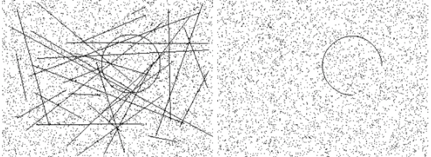
We also make other experiments using two binary image sequences, as shown in Figure 6. In the first case (Figure 6 (left)), we use a circular arc, which lacks part of the circle, as the target to be tracked. In the second case (Figure 6 (right)), we create the images having the more cluttered background than that of the first experiment; we add 20 line segments whose end-points are generated from the uniform distribution over the image plane. In both of the experiments, the other conditions, such as the target transition in Eq. (17) and the number of the background noises, are the same as the first experiment. The experimental results show that the proposed algorithm successfully tracks the circle even if the occlusion occurs or the background becomes cluttered.

7.

CONCLUSIONS

A visual tracking algorithm based on hypothesis propagation and voting-based verification is proposed. The proposed algorithm detects a curve in binary images by evaluating the curve by its received votes, and propagates the detected curve to the successive image of a given sequence. Although voting-based algorithms, such as the Hough transform and RANSAC, in general, are

(9)

time-consuming, this propagation over time provides an efficient search procedure for finding curves. In addition, a procedure for preventing redundant verification by determining equivalence curves in the digital space is introduced. This procedure contributes to the improvement of the efficiency of the algorithm. The experimental results show the execution time decreases by 32.9% when the particles are 10000 in number. Thus, two combinations of hypothesis propagation and voting-based verification enable us to track curves in clutter robustly and efficiently. Furthermore, a particle elimination procedure to suppress rapid diffusion of particles over time is introduced, which phenomenon is likely to happen in clutter. As a result, the elimination procedure prevents the variance of the filtering distribution from increasing over time.

It might be worth mentioning those which should be developed in the future. The paper assumes that transition model of target objects (e.g., Eq. (10)) is known. Then, if the object moves unexpectedly, the algorithm is likely to fail to track it. An adaptive or self-organized process may be useful for treating such a situation.

Robust and efficient algorithms in image processing and computer vision are strongly required in academic and industry because of the spread of computers and digital cameras. The proposed algorithm gives a basis of such image and vision technologies.

ACKNOWLEDGEMENTS

This work was supported in part by the Ministry of Education, Culture, Sports, Science and Technology, Japan, under a Grant-in-Aid (No.16700169).

REFERENCES

[1] R. O. Duda and P. E. Hart, “Use of the Hough transformation to detect lines and curves in pictures,” Comm. ACM, Vol. 15(1), pp. 11-15, 1972.

[2] M. A. Fischer and R. C. Bolles, “Random sample consensus: a paradigm for model fitting with applications to image analysis and automated cartography,” Comm. ACM, Vol. 24(6), pp. 381-395, 1981.

[3] J. P. Princen, J. Illingworth, and J. V. Kittler, “A Formal Definition of the Hough Transform: Properties and Relationships,” J. Mathematical Imaging and Vision, Vol. 1, No. 1, pp. 153-168, 1992.

[4] J. Bresenham, ”A Linear Algorithm for Incremental Digital Display of Circular Arcs,” Comm. ACM, Vol. 20(2), pp. 100-106, 1977.

[5] L. Xu and E. Oja, “Randomized Hough Transform: Basic Mechanisms, Algorithms and Computational Complexities,” CVGIP: Image Understanding, Vol. 57(2), pp. 131-154, 1993.

[6] J. R. Bergen and H. Shvaytser, “Probabilistic Algorithm for Computing Hough Transform,” J. Algorithms, Vol. 12(4), pp. 639-656, 1991.

[7] N. Kiryati, Y. Eldar, and M. Bruckstein,” A Probabilistic Hough Transform,” Pattern Recognition, Vol. 24(4), pp. 303-316, 1991. [8] O. Chum and J. Matas, “Randomized

RANSAC with

T

d,d test,” Proc. the British

Machine Vision Conference, Vol. 2, pp. 448-457, 2002.

[9] A. Rosenfeld, J. Jr. Ornelas, and Y. Hung, “Hough Transform Algorithms for Mesh-Connected SIMD Parallel Processors,” Computer Vision, Graphics, and Image Processing, Vol. 41(3), pp. 293-305, 1988.

[10] H. Li, M. A. Lavin, and R. L. Master, “Fast Hough transform: a hierarchical approach,” Computer Vision, Graphics, and Image Processing, Vol. 36, pp. 139-161, 1986. [11] J. Illingworth and J. Kittler, “The adaptive

Hough transform,” IEEE Trans. Pattern Analysis and Machine Intelligence, Vol. 9(5), pp. 690-698, 1987.

[12] P. H. S. Torr, and C. Davidson, “IMPSAC: synthesis of importance sampling and random sample consensus,” IEEE Trans. Pattern Analysis and Machine Intelligence, Vol. 25(3), pp. 354-364. 2002.

[13] J. S. Liu and R. Chen, “Sequential Monte Carlo methods for dynamic systems',” J. the American Statistical Association, Vol. 93, pp. 1033-1044, 1998.

[14] A. Doucet, S. Godill, and C. Andrieu, “On Sequential Monte Carlo Sampling Methods for Bayesian Filtering,” Statistics and Computing, Vol. 10(3), pp. 197-208, 2000. [15] A. Doucet, N. de Freitas, and N. J. Gordon,

“Sequential Monte Carlo Methods in Practice,” Springer-Verlag, 2001.

(10)

[16] N. J. Gordon, D. J. Salmond, and A. F. M. Smith, “Novel approach to nonlinear/non-Gaussian Bayesian state estimation',” IEE Proc. F, Vol. 140(2), pp. 107-113, 1993.

[17] M. Isard and A. Black, “Condensation - Conditional density propagation for visual tracking,” Int. J. Computer Vision, Vol. 29(1), pp. 5-28, 1998.

[18] M. S. Arulampalam, S. Maskell, N. Gordon, and T. Clapp, “A Tutorial on Particle Filters for Online Nonlinear/Non-Gaussian Bayesian Tracking',” IEEE Trans. Signal Processing, Vol. 50(2), pp.174-188, 2002. [19] G. Kitagawa, “Monte Carlo filter and

smoother for non-Gaussian nonlinear state space models,” J. Comput. Graph. Stat., Vol. 5(1), pp.1-25, 1996.

[20] W. H. Press, S. A. Teukolsky, W. T. Vetterling,”Numerical Recipes in C: The Art of Scientific Computing,” Cambridge University Press, 1993.

AUTHOR INFORMATION

Kazuhiko Kawamoto received his M.E. and Dr.E. degrees in information science from from Chiba University, Japan, in 1999 and 2002, respectively. From 2002 to 2005, he was an assistant professor at the

Department of Computational Intelligence and Systems Science,

Tokyo Institute of Technology, Japan. Since 2005, he has been an associate professor at Faculty of Engineering, Kyushu Institute of Technology, Japan. His recent research interests include computer vision and pattern recognition.

Kaoru Hirota received his M.E. and Dr.E. degrees in electronics from Tokyo Institute of Technology, Japan, in 1976 and 1979, respectively. From 1979 to 1982, he was with the Sagami Institute of Technology, Japan. From 1982 to 1995, he was with Hosei University, Japan. Since 1995, he has been a professor at the Department of Computational Intelligence and Systems Science, Tokyo Institute of Technology, Japan. His research interests include broad-ranging fields in soft computing.