Shippey, Thomas, Bowes, David and Hall, Tracy
Available at http://clok.uclan.ac.uk/24433/
Shippey, Thomas, Bowes, David and Hall, Tracy (2018) Automatically Identifying Code Features for Software Defect Prediction: Using AST N-grams. Information and Software Technology . ISSN 0950-5849
It is advisable to refer to the publisher’s version if you intend to cite from the work.
http://dx.doi.org/10.1016/j.infsof.2018.10.001
For more information about UCLan’s research in this area go to
http://www.uclan.ac.uk/researchgroups/ and search for <name of research Group>.
For information about Research generally at UCLan please go to http://www.uclan.ac.uk/research/
All outputs in CLoK are protected by Intellectual Property Rights law, including
Copyright law. Copyright, IPR and Moral Rights for the works on this site are retained by the individual authors and/or other copyright owners. Terms and conditions for use
of this material are defined in the http://clok.uclan.ac.uk/policies/
CLoK
Accepted Manuscript
Automatically Identifying Code Features for Software Defect Prediction: Using AST N-grams
Thomas Shippey, David Bowes, Tracy Hall
PII: S0950-5849(18)30205-2
DOI: https://doi.org/10.1016/j.infsof.2018.10.001 Reference: INFSOF 6057
To appear in: Information and Software Technology
Received date: 20 February 2018 Revised date: 4 September 2018 Accepted date: 2 October 2018
Please cite this article as: Thomas Shippey, David Bowes, Tracy Hall, Automatically Identifying Code Features for Software Defect Prediction: Using AST N-grams,Information and Software Technology (2018), doi:https://doi.org/10.1016/j.infsof.2018.10.001
This is a PDF file of an unedited manuscript that has been accepted for publication. As a service to our customers we are providing this early version of the manuscript. The manuscript will undergo copyediting, typesetting, and review of the resulting proof before it is published in its final form. Please note that during the production process errors may be discovered which could affect the content, and all legal disclaimers that apply to the journal pertain.
ACCEPTED MANUSCRIPT
Automatically Identifying Code Features for Software Defect
Prediction: Using AST N-grams
Thomas Shippeya, David Bowesb, Tracy Hallc
aUniversity of Hertfordshire
bUniversity of Central Lancashire
cLancaster University
Abstract
Context: Identifying defects in code early is important. A wide range of static code metrics have been evaluated as potential defect indicators. Most of these metrics offer only high level insights and focus on particular pre-selected features of the code. None of the currently used metrics clearly performs best in defect prediction.
Objective: We use Abstract Syntax Tree (AST) n-grams to identify features of defective Java code that improve defect prediction performance.
Method: Our approach is bottom-up and does not rely on pre-selecting any specific features of code. We use non-parametric testing to determine relationships between AST n-grams and faults in both open source and commercial systems. We build defect prediction models using three machine learning techniques.
Results: We show that AST n-grams are very significantly related to faults in some systems, with very large effect sizes. The occurrence of some frequently occurring AST n-grams in a method can mean that the method is up to three times more likely to contain a fault. AST n-grams can have a large effect on the performance of defect prediction models.
Conclusions: We suggest that AST n-grams offer developers a promising approach to iden-tifying potentially defective code.
1. Introduction
The aim of this paper is to automatically identify features of faulty Java code and use these features to improve defect prediction performance. Our approach is based on analysing the Abstract Syntax Tree (AST) for a piece of code. AST n-grams are sets of Java AST nodes. These AST n-grams define the low level programming constructs that have been used in a piece of code and the order in which these are used. We analysed the code to
Email addresses: [email protected](Thomas Shippey),[email protected] (David Bowes),
[email protected](Tracy Hall)
This work was partly funded by a grant from the UK’s Engineering and Physical Sciences Research Council under grant number: EP/L011751/1. We would like to thank our collaborator for allowing us to use their source code, defect repository and version control systems.
ACCEPTED MANUSCRIPT
identify AST n-grams in nine open source systems and two commercial telecommunication
Java systems. We report many AST n-grams that are significantly associated with faults1
across all eleven systems. We show that including AST n-grams in defect prediction models improves predictive performance.
Traditionally studies have focused on investigating which static features of code are associated with defects [31]. These previous approaches are top-down, focusing on a partic-ular pre-selected set of code features, for example features associated with coupling or size. Many other features of code that may be fault-prone are not considered in such top-down approaches. The performance of these traditional defect prediction models seems to have reached a performance ceiling [49]. In response to this ceiling a new bottom-up approach to identifying the defective features of code is emerging. This approach automatically learns the defective features of code by analysing the semantics of the code via the Abstract Syn-tax Tree. Wang et al. [71] built promising defect prediction models based on a subset of AST nodes using neural networks. Pradel and Sen [55] also used a neural network to build good defect prediction models using a sub-set of AST nodes (those based on identifiers and literals). We extend both of these previous studies by analysing the full set of AST nodes in relation to defects, rather than only the limited sub-set of features previously investigated. We report important new code features related to defects. We also go further by reporting our results at method rather than class level and evaluating our approach on an extended set of projects including two closed source projects. We identify features of code not used in defect prediction previously and which have large effects on the performance of defect prediction models.
Our approach starts by serialising a Java method’s AST. For each method, a serialisation is created by using a pre-order traversal of the AST, with the ordering being determined by the sequence in which the nodes are visited. AST n-grams are then extracted from the
method serialisation. These AST n-grams are an n-gram2 of the serialised AST, where an
n-gram unit is a node of the AST. These AST n-grams capture the low level building blocks that have been used in the code and, so, provide comprehensive fine grained insight into the features of that code.
We investigate and quantify the relationship between AST n-grams and faults, by an-swering the following research questions:
Research Question 1: Are any AST n-grams significantly associated with faulty code? Research Question 2: What is the effect size of AST n-grams significantly associated with faulty code?
Research Question 3: Does the inclusion of AST n-grams that are significantly associated
1We use the IEEE definition [35] of a fault being a reported defect, where a defect is a mistake in code
made by a developer which may result in a failure of the program to execute as planned.
2An n-gram is a term we have taken from computational linguistics describing a contiguous subset of a
ACCEPTED MANUSCRIPT
with faults in defect prediction models improve the performance of these models?
We answered the first two research questions by analysing five different systems and, to guard against overfitting, we added six systems for the third research question. In total there are nine open source systems and two commercial telecommunication systems. Using the Java AST, we extracted the AST n-grams from each system and used the SZZ [67] algorithm to identify faulty methods. We then used non-parametric tests to identify significant rela-tionships between AST n-grams and faults in Java methods. We calculated the effect size of the significant relationships found. Finally, we performed defect prediction on all systems, creating models with the AST n-grams significantly associated with faults, and models with-out. We compared these models to determine if there was a significant difference between the performance. As a baseline, we also compared our models, which are built with all the possible AST nodes, with the reduced set used by Wang et al. [71]. Our approach differs slightly from Wang et al. [71] as our analysis focuses on the type of AST nodes rather than the contents of those nodes. Wang et al. [71] provide node content analysis for a small set of nodes (names of methods and variables). Our analysis de-emphasises node contents as Wang et al. [71] reported that their node content analysis produced project and developer-specific findings are not generalisable.
Our results make three contributions:
Contribution 1. We present an automatic code analysis technique that comprehen-sively and objectively serialises all low level code constructs used in a software system. Specifically we introduce the concept of a method serialisation and n-gram of this serialisa-tion called an AST n-gram. This analysis technique allows researchers and practiserialisa-tioners to better understand the structure of the code in individual systems.
Contribution 2. We present important new evidence on fault-prone code constructs. We identify relatively common code structures which can make a method four times as likely to be fault-prone. We identify two code structures which involve identifiers which are fault-prone across all five systems we investigate. This new evidence of fault-prone code structures provides researchers and practitioners with new information with which to strengthen existing defect reduction approaches.
Contribution 3. We show that the inclusion of AST n-grams in within-project software defect prediction models significantly improves the performance of models built using source code metrics. Performance improves when AST n-grams significantly associated with faults are added to the models. This improvement can be up to 4.6 times that of the model con-structed with just source code metrics. This means that we could find up to 4.6 times more defects using AST n-grams. Our findings can improve the effectiveness of defect prediction and also in the future could be integrated into developer IDE’s (Integrated Development Environments) to reduce faults being initially introduced into code, or efficiently direct testing.
The rest of this paper is structured as follows: Section 2 describes related work. Section 3 outlines how we conducted our investigation and Section 4 presents results. Section 6 we highlight related work and we note the potential threats to validity in Section 5. In Section 7 we discuss the implications of our findings. Finally we conclude in Section 8.
ACCEPTED MANUSCRIPT
2. Background
Software defect prediction uses machine learning to determine potentially defective areas in software code. The predictions make it possible for the developer to focus on areas of the software system before release, reducing the time and effort of finding defects by other means. Software defect prediction relies on three main components; dependent variables, in-dependent variables and a model. Dependent variables are the defect data for the particular piece of code (i.e. is it defective or not), which can be binary, or continuous. Independent variables are the metrics which can describe the software code, how it has changed or who changed it. Independent variables come in two forms, software code metrics; those that can be derived from the software code itself, and process metrics; metrics that measure the change of software code or software practices over time. The model contains the rule(s) or algorithm(s) that predict the dependent variable from the independent variables. These rules can be as simple as the number of independent variables in the model, or be as
com-plicated as decision trees3 and regression4 techniques. To determine the effectiveness of the
model, the variables are split into test and training sets. Where the training set is used to create a model and that model is then used on the test set to predict potential defects. These predictions are then investigated to determine if they are correct or not by certain performance measures.
Previous work on features of code in relation to defects is focused on defining and evalu-ating source code metrics (SCM) that measure particular code features. Examples of source code metrics include - lines of code, object oriented metrics and McCabe’s complexity met-rics. Various studies have measured source code using such metrics and looked at how the code features measured relate to defects [6, 78, 46, 51, 33, 41, 73].
Lines of code (LOC) is a simple measure that has been commonly used to indicate where defects are. For example, Fenton and Ohlsson [22] analysed pre and post release defects of a large communications system. They found that LOC was good at ranking defective methods. LOC has been used in many other studies [78, 8, 30, 76, 38] and has been reported to be good at predicting defective code [31]. However LOC measures only one coarse grained feature of code and so provides limited insight into potential sources of defects.
Chidamber and Kemerer (CK) developed six Object Oriented (OO) metrics to measure the object oriented features of code (e.g. Coupling, Depth of Inheritance Trees and Weighted Methods per class). These metrics have been successfully used in studies to identify defective code [4, 11, 39, 15, 19]. Although, compared to LOC, the CK metrics do measure some finer grained features of code, and also identify more of those features, they still identify only a fixed subset of possible code features.
McCabe’s cyclomatic complexity metric [44] focuses on identifying branching structures in code and measuring the number of logical paths though the code. Other forms of cyclo-matic complexity have been proposed [81, 23]. Cyclocyclo-matic Complexity is another commonly
3A decision tree algorithm is one that creates a graph of decisions based on the chance of an event
happening.
ACCEPTED MANUSCRIPT
used metric in defect prediction studies with mixed success (e.g. studies [48, 69, 47]). How-ever, again, when used in defect prediction Cyclomatic Complexity focuses only on a small set of pre-determined code features likely to be related to defects.
Most of the traditional SCMs (above) have been extensively used in previous defect prediction studies [31]. Most of these metrics suffer from being very coarse grained and with capability to measure only a small sub-set of code features. Gray et al. [29] suggest that the coarse grained nature of such metrics prevents machine learning techniques from effectively differentiating between defective and non-defective methods: if one method has the same metric values as another (say in terms of LOC), but they have not been labelled the same in terms of their defectiveness, this will hinder the learning algorithm’s ability to
learn. Gray et al. [29] identifies many methods in the NASA datasets5 which have identical
values across a range of metrics but different defectiveness labels. This suggests that the current commonly used set of metrics is not sufficient to differentiate methods for defect prediction.
Complexity and size are code features commonly used in defect prediction [48, 69, 47]. Despite much effort in identifying and evaluating such features of code, there is no static code feature which consistently identifies problematic code across systems [48, 31]. Code features that indicate defects are usually system-specific [80]. Combinations of features have, so far, performed most promisingly in defect prediction. For example, Shivaji et al. [66] used combinations of static code metrics, object oriented metrics, churn metrics and textual features while Bird et al. [11] used combinations of developer contribution network metrics. Unfortunately, collecting data for such combinations is difficult, time consuming and costly. Furthermore, the ability of such combinations to identify defects, relies on the performance of each single feature included in the combination. Therefore, it is important to be able to identify features indicative of defective code and to develop associated code analysis techniques to identify these features.
Defect predictions are usually reported in studies at the package, class or file level of granularity (e.g. [52], [4]). Hata et al report that predictions at this relatively high level of granularity are not necessarily useful to developers [34] and that predictions at lower levels of granularity are likely to be most useful to developers. Such low granularity predictions (e.g. at method level) present developers with fewer lines of code in which to locate the predicted defect. Locating the predicted defect is often via manual inspection and so the fewer the lines of code to be inspected the less developer time is wasted searching for the defect. Giger et al [26] report good predictive performance at method level using both change metrics and source code metrics. However achieving good predictive performance at the method level is not easy. Indeed Pascarella et al [54] replicated [26] with a release-based performance evaluation strategy but reported poor predictive performance at method level. Despite a growing preference for method-level defect prediction, it remains an open challenge to build defect prediction models at method level [54]. We are amongst the few studies reporting defect predictions at method level and the performances that we report are competitive to studies reporting at higher levels of granularity.
ACCEPTED MANUSCRIPT
3. Methodology
To identify AST n-grams of Java code which are associated with faulty methods we collected data about which methods were faulty. We also needed to know which set of Java AST n-grams each method contained. We used statistical techniques to identify which AST n-grams are significantly associated with faulty and with non faulty methods of code. We finally include the AST n-grams that are significantly associated with faulty methods of code to defect prediction models and compare performance of those models, to models formed with the reduced AST n-gram set proposed by Wang et al. [71].
3.1. Open Source and Commercial Datasets
The open source Java systems analysed in this study were chosen because they have already been extensively used in defect prediction studies [31]. Although we collected fault data ourselves, we chose Eclipse.JDT.core 3.0 because the faults for this system had previously been mapped between the bug tracking system and the version control system [67, 10, 40]. Using a system which had been analysed for faults previously allowed us to val-idate our own technique for locating code that was faulty. We also analysed major releases of ArgoUML 0.20 and AspectJ 1.7.0 because they were Java solutions to different problems and had also been previously studied [57, 18, 72]. We also collected fault data from two com-mercial telecommunications systems. The code, together with raw bug tracking and version control data was provided to us by a large international telecommunications company based in the UK. The contextual information for each system can be found in Table 1. During the software defect prediction phase of this work, we added six more systems (shown in Table 1). We added these extra systems because we wanted to be sure that the defect prediction results we had for the first five systems would be sustained in other open source systems. These systems were chosen as our previous work had shown them to have sufficient defects to perform defect prediction [65].
System Release KLOC Total Methods
EJDT 3.0 292 13,885 ArgoUML 0.20 273 12,330 AspectJ 1.7.0 353 21,980 T1 - 52 3,914 T2 - 36 4,896 JMRI 2.4 550 19,861 SocialSDK 1.1.8.2015 69 10,183 GenoViz 5.4 193 8,489 JBoss Reddeer 1.2 38 6,475 K Framework 3.6 39 5,297 JMOL 6 225 2,269
Table 1: The 11 systems analysed in this paper. The T2 and T1 release number is the revision number before the systems were put into production.
ACCEPTED MANUSCRIPT
3.2. Identifying which methods are faultyFor each of the systems we compiled a dataset of faulty methods. We found which methods were faulty at the time of release by finding the fault insertion and fix points. To identify faulty methods we used the SZZ approach as it has been used in many previous
studies [16, 24, 40, 41, 74, 79]. SZZ is a fault linking algorithm described by ´Sliwerski,
Zimmermann, and Zeller [67]. SZZ was based on work by Cubranic and Murphy [16] and Fischer et al. [24], who inferred links between Bugzilla defect reports with CVS commit messages. The SZZ algorithm matches the fault fix described in a bug tracking system with the corresponding commit in a version control system that ‘removed’ the fault. By backtracking through the version control records, it is possible to identify earlier code changes which ended up being ‘fixed’. It is assumed that the earlier code changes inserted the fault. The method of code is therefore labeled as faulty between the time the fault was inserted and the time it was fixed. Using this technique it is possible to identify for a particular snapshot of the code base, which methods are faulty and which are not. If there are multiple changes multiple times in the past, we assume that the fault inducing change is the one immediately before the defect report. The method is marked as defective if the version snapshot lies between the fault inducing commit and the fault fixing commit and there is no change between these two commits. The tool we have created tracks individual lines throughout the history of the project to determine which methods are defective at a particular time. More details about our tool can be found in [65].
There will be defective methods which have not yet been reported. It is therefore im-portant to carry out the fault mapping after sufficient time has passed for users to report most faults. It is unlikely that all defects will be reported and therefore there will be false negatives. Kim et al. [42] suggests that as long as the number of false negatives and false positives is less than 20% in total, defect prediction can be carried out [42]. This is an important point, early work by Zimmermann et al. [79] only managed to map about 50% of faults reported in the bug tracking systems to changes in the code base. Later Bird et al. [10] improved the mapping by removing some of the constraints that Zimmermann had intro-duced, for example the requirement to have matching bug IDs in a predefined format. The implementation of SZZ used in this paper was improved slightly from the original. It has a higher weighting for those numbers found in commit messages that are in the bug database and takes into account the “Fix for” prefix. The implementation was verified by manually checking ALL bug links found for EJDT 3.0. Table 2 shows that the implementation used in this study has 80% recall and 99% precision.
Alencar da Costa et al [17] recently evaluated the SZZ variants used in studies and our variant falls into Alencar da Costa et al’s L-SZZ category. This is because not only does our tool use annotation graphs to achieve line mappings and is aware of meta changes but also identifies the largest bug introducing change. Approaches in the L-SZZ category are currently most mature in identifying bug introducing changes.
Table 3 shows the defectiveness of each of the systems studied in our experiment. The levels of fault-proneness varies across all systems. T2 has the highest fault density with over 12% defective methods, followed by the second telecommunications system T1 with around 9%. AspectJ has only 19 methods faulty out of a potential 21,980 and so has a very low
ACCEPTED MANUSCRIPT
This Paper Zimmermann et al. [79]
True Positive 727 483 False Positives 5 2 Total Positives 732 485 Total Negatives 151 398 Recall 80% 53% Precision 99% 100%
Table 2: Checking the bug-links for false positives. Zimmermann has similar precision but lower recall.
Precision is the proportion of correctly classified bug-links from all those bug-links classified (T P/(T P+F P))
and recall is the proportion of bug-links correctly classified from all possible correct bug-links (T P/(T P +
F N))
System Version Total Methods Faulty Methods % Faulty
T2 198468 4,896 612 12.5 T1 198468 3,914 360 9.2 EJDT 3.0 13,885 589 4.24 ArgoUML 0.20 12,330 42 0.34 AspectJ 1.7.0 21,980 19 0.09 JMOL 6 2,269 294 12.96 GenoViz 5.4 8,489 827 9.63 K Framework 3.6 5,297 421 7.95 SocialSDK 1.1.8.2015 10,183 754 7.40 JMRI 2.4 19,861 1,385 6.97 JBoss Reddeer 1.2 6,475 416 6.42
Table 3: Table to show the fault density of each of the datasets. N.B. Tables have been presented in order of percentage faulty.
fault-proneness of 0.09%.
3.3. Extracting the Java AST n-grams
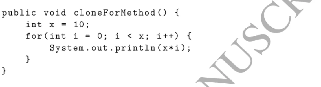
For each of the systems investigated, each file in the project was compiled using the Oracle JDK which builds an AST. Each method in a class was turned into a method sequence using
a modified version of the standard Oracle Java pretty printer6. A method sequence is a list
of AST nodes in order of when they are visited by the pretty printer, which is a pre-order depth first traversal. The pretty printer uses a visitor pattern to transforms the source code by applying styling rules (e.g. appropriate indents and spacing), which can make it easier for people to view. We modified the pretty printer so when it visits a node on the AST, it will store that node in a sequence. This means that the order in which code constructs are visited is maintained. For example, we would transform the piece of Java source code in Figure 1 into the method sequence in Figure 2. This method was used to transform all
ACCEPTED MANUSCRIPT
System Version Total Sequences Avg
Sequence Length Sequence σ Max Sequence Length T1 198468 3,914 19.73 21.88 351 T2 198468 4,896 24.00 25.87 386 EJDT 3.0 13,885 55.47 129.64 4,802 ArgoUML 0.20 12,330 36.04 68.61 2,989 AspectJ 1.7.0 21,980 37.79 75.18 2,644
Table 4: Table to show the sequence statistics for each of the systems analysed. The minimum sequence length for all systems was three. A sequence of length three is found for zero argument empty constructors
e.g. public Foo()N.B. Tables have been presented in order of percentage faulty.
public void c l o n e F o r M e t h o d () { int x = 10;
for ( int i = 0; i < x ; i ++) { System . out . println ( x * i ); }
}
Figure 1: The code that is transformed in Figure 2 using the Pretty Printer.
methods in the five systems to create a database of method sequences. Table 4 shows how many methods were transformed into method sequences and the average length of these method sequences. Method sequence lengths vary across the system, with EJDT 3.0 having the longest average by around 20 nodes. The commercial systems have both a lower average sequence length and maximum sequence length. This is because the company has a policy of keeping both classes and methods as short as possible.
From our method sequences, we can extract n-grams, which we call“AST n-grams”. We
extract from each method AST n-grams which are 1-gram, 2-gram and so on, up until the maximum length of n-grams. For example, we want to extract the AST n-grams from an
example sequence (M)[A; A; C; D; E] where the maximum AST n-gram length is three.
In total the setCS contains 11 AST n-grams. Figure 3 shows the AST n-grams in setCS.
For this study we have set the maximum AST n-gram length to seven. This is because as an AST gram length gets longer, there is an exponential increase in the number of AST
n-METHOD ; M O D I F I E R S ; P R I M I T I V E _ T Y P E ; BLOCK ; V A R I A B L E ; M O D I F I E R S ; P R I M I T I V E _ T Y P E ; I N T _ L I T E R A L ; F O R _ L O O P ; V A R I A B L E ; M O D I F I E R S ; P R I M I T I V E _ T Y P E ; I N T _ L I T E R A L ; L E S S _ T H A N ; I D E N T I F I E R ; I D E N T I F I E R ; E X P R E S S I O N _ S T A T E M E N T ; P O S T F I X _ I N C R E M E N T ; I D E N T I F I E R ; BLOCK ; E X P R E S S I O N _ S T A T E M E N T ; M E T H O D _ I N V O C A T I O N ; M E M B E R _ S E L E C T ; M E M B E R _ S E L E C T ; I D E N T I F I E R ; M U L T I P L Y ; I D E N T I F I E R ; I D E N T I F I E R ;
ACCEPTED MANUSCRIPT
CS = {( A ) , ( A ; A ) , ( A ; A ; C ) , ( A ; C ) , ( A ; C ; D ) , ( C ) , ( C ; D ) , ( C ; D ; E ) , ( D ) , ( D ; E ) , ( E ) }
Figure 3: The possible set of 11 AST n-grams (with a maximum n-gram of three) taken from an example
method sequenceA; A; C; D; E
Faulty Non-Faulty Total
N-gram 32,493 7,750 40,243
(%) 80.74 19.26
-No N-gram 230,681 4,311,566 4,542,247
(%) 0.05 95.5
-Total 263,174 4,319,316 4,582,490
Table 5: Contingency Table for AST n-gram METHOD INVOCATION MEMBER SELECT in EJDT 3.0 grams available. The limit of seven nodes prevented potential computational problems when we came to analysing the results. We do not extract the contents of the AST n-grams as our analysis is at the type level of granularity rather than the instance level of granularity. This means that our results are less influenced by the particular coding idiosyncrasies of individual developers in individual projects. Our aim is to present results that are more likely to be generalisable.
3.4. Analysing the AST n-grams
To find which AST n-grams are related to faults we compare the ratio of n-grams in non faulty code to the number of n-grams in faulty code. In this study we compare the number of instances of an AST n-gram. An n-gram is marked as faulty if it appears in a faulty method at the chosen snapshot. As the distribution of AST n-grams is normal we used the non-parametric Fisher’s exact test to determine if an AST n-gram was significantly associated with a fault. Fisher’s exact test determines if there are non-random associations between two categorical variables. In our case, the classifications are the presence or absence of a n-gram and faulty or not. To clarify our statistical analysis, we provide a worked example using EJDT 3.0. In EJDT 3.0 there is a 2.65% chance of any AST n-gram being defective. This is determined by dividing the number of faulty AST n-gram instances over all AST n-gram instances. The contingency table (Table 5) is for the AST n-gram METHOD INVOCATION MEMBER SELECT. This AST n-gram is the start of a method call. Our null hypothesis is that METHOD INVOCATION MEMBER SELECT appears in the same proportion of faulty n-grams as non-faulty n-grams. Our alternate hypothesis is that the AST n-gram appears in a greater proportion of faulty n-grams than non-faulty n-grams. When the Fisher’s exact test is applied to the contingency table in Table 5 we get a p-value of 0.0.
This is below ourα of 0.001. This means there is evidence to reject the null hypothesis. We
would conclude that the start of a method call in EJDT 3.0 is significantly associated with
faults. We set our α to 0.001 as we wanted to reduce the amount of false positives when
ACCEPTED MANUSCRIPT
We have calculated the effect sizes for the AST n-grams significantly associated with faults using an odds-ratio [14]. The odds-ratio will quantify how strongly the presence of an AST n-gram will be associated with a fault. The odds-ratio has a range of zero to infinity. If the odds-ratio is less than one, then the n-gram may be more associated with non-faults. When the odds-ratio is one then that means that the AST n-gram does not have any effect on the fault proneness of the code. The greater the amount away from one, the greater the effect that the AST n-gram has on the association with faults.
3.5. Defect Prediction using the AST n-grams 3.5.1. Building the defect prediction models
To answer RQ3, we carried out defect prediction using the AST n-grams. To show that the significant AST n-grams were having an effect, we created basic defect prediction models without the AST n-grams. These models were created with the default set of static code
metrics calculated by the program JHawk7. These metrics include lines of code (LOC),
variable declarations and Halstead metrics. In total there are 27 method level metrics and the full list of software code metrics used can be found in Appendix A. We then added the AST n-grams significantly associated with faults, up until a maximum of 200 n-grams. We chose a maximum 200 AST n-grams due to computational constraints. Adding attributes to models has an exponential computational time costs when building the model. These increased costs vary from learner to learner with high costs associated with, for example, Random Forest learners but minimal cost increases associated with Na ive Bayes.
In total, we had 11 metric datasets per classifier for each system, one metric dataset with just JHawk metrics, and then 10 more metric datasets with AST n-grams significantly asso-ciated with faults as additional attributes. When we added the AST n-grams as attributes to the models, we used the binary presence of an n-gram, not the number of n-grams in a method. We used the binary value rather than total as binary values are standard in defect prediction. Our approach of adding AST n-grams to a base of existing source code metrics increases the information available to the defect prediction model. Increasing information diversity has been previously shown to improve predictive performance (e.g. [31]) and in-crementally adding information to the model is being increasingly used in defect prediction research (e.g. [12]).
3.5.2. Training the models using AST n-grams
To determine which AST n-grams to add as attributes to our initial baseline model, we calculated the top 200 most occurring AST n-grams significantly associated with faults at the 99.9% level only from methods in the training set for each run and fold. We calculated the significant AST n-grams in only each training set to make sure that when testing our models they did not have any prior knowledge of the significant AST n-grams. For each run and fold, we created 10 models per classifier to compare with the original model. From zero up to 50 n-grams, we added an additional 10 significant n-grams to the metric dataset and trained the model on this new dataset, after 50 we increased the additional number of
ACCEPTED MANUSCRIPT
Number of Significant N-grams
Model # JHawkMetrics 10 20 30 40 50 75 100 125 150 175 200 0 X × × × × × × × × × × × 1 X X × × × × × × × × × × 2 X X X × × × × × × × × × 3 X X X X × × × × × × × × 4 X X X X X × × × × × × × 5 X X X X X X × × × × × × 6 X X X X X X X × × × × × 7 X X X X X X X X × × × × 8 X X X X X X X X X × × × 9 X X X X X X X X X X × × 10 X X X X X X X X X X X × 11 X X X X X X X X X X X X
Table 6: The number of significant n-grams in each of the 11 comparison metric datasets.
AST n-grams by 25 until we reached 200. So the first model would be trained using the initial JHawk metrics only, then second model uses the JHawk metrics plus the top ten most occurring AST n-grams significantly associated with faults in the training set and the third model would have the top 20 and so on, until 50 AST n-grams. After 50 n-grams, the models would be trained with an additional 25 AST n-grams, so the next model after 50 is 75 n-grams, then 100, then 125 and so on. Until the last comparison model had the top 200 most frequently occurring AST n-grams that were significantly associated with faults in that particular training set. Our analysis suggests that generally the more n-grams provided the more defect prediction performance improves. However this is not always the case and identifying the particular combinations of n-grams that work best for particular data sets/projects improves performance most. Song et al [68] also notes the need to tailor features to projects to achieve good predictive performance. Table 6 shows how many AST significant n-grams are in each of the 11 models.
3.5.3. Cross validation scheme
Each dataset was split into ten stratified folds to perform cross validation. Each fold was held out in turn to produce a test set and the other folds were used to produce the training set. Using stratified cross validation ensures that there are instances of the defective class in each test set, thus reducing the likelihood of classification uncertainty. The classifiers were trained using the training sets and the test set then used to evaluate the model. This experiment was repeated 100 times for each classifier and system dataset. We chose 100, instead of the more common 10 times, as Mende [45] reports that using 10 experiment repeats results in an unreliable final performance figure. This meant that we determined the top 200 AST n-grams that are significantly associated with faults in 1,000 training sets
and computed 33,000 models per system8.
ACCEPTED MANUSCRIPT
3.5.4. Classifier selectionWe created our models using three classifiers: Na¨ıve Bayes, J489, and Random Forest.
Bayes classifiers are simple probabilistic classifiers based on applying Bayes’ theorem. Na¨ıve Bayes is the most popular Bayes classifier. Na¨ıve Bayes is called naive since every feature (module) is assumed to be fully independent. Na¨ıve Bayes will produce models based on the combined probabilities of a dependent variable being associated with the different indepen-dent variables. J48 and Random Forest use decision tree learning. Decision tree learning uses a decision tree as a predictive model to map observations to a target value. Decision trees that only take a finite set of values are called classification trees. The J48 classifier builds decision trees based on the information gain of attributes. At a node in the tree, the J48 algorithm will chose the attribute of the data that most effectively splits the set into subsets enriched in one class or another. The split is based upon the attribute with the highest normalised information gain. This then repeats on the smaller subsets until the tree is built. Random Forest is an ensemble technique which aggregates the predictions made by a collection of decision trees. Each of the trees is said to be randomised as they train on a subset of available features. The mode classification across all individual classifiers is taken as the final prediction for each test vector (method). We chose these three classifiers because they are popular modelling classifiers according to Hall et al. [31]. We built the
models using a Java implementation of Weka10 using the default options for each classifier.
3.5.5. Predictive performance
We calculated each model’s performance using four different measures: precision, recall, f-measure and Matthew’s correlation coefficient (MCC). See Table 7 for definitions of these measures. Precision, recall and f-measure were chosen as they are very commonly published in defect prediction papers, and have a range of 0 to 1, with 0 being no better than random prediction and 1 being perfect prediction. MCC was chosen because it is easy to understand and includes all four components of the confusion matrix. MCC has a range of -1 to 1, with 1 being perfect prediction and -1 being total disagreement. An MCC score of 0 means the performance is no better than a random prediction.
We will statistically compare what effect the addition of AST n-grams has on our models. Our hypothesis is that models trained using AST n-grams will perform better than ones that do not contain AST n-grams significantly associated with faults. We used the Wilcoxon signed-rank test to compare the differences in performance measurements from the 100 runs of the models with the significant AST n-grams to those without. We have used the Wilcoxon signed-rank test as our data does not follow the normal distribution and is paired. Our data is paired as we have calculated the performance measurement for each run and fold (and the methods in each run and fold are always the same). We calculated the effect size of each test using Cliff’s delta. We again have used Cliff’s delta as our data is not normally distributed. We calculated the effect size to show the level of impact the AST n-grams had
on the performance of our models. Cliffs delta(d) gives a score between -1 and 1, with± 1
9J48 is the Weka implementation of the C4.5 algorithm.
ACCEPTED MANUSCRIPT
Measure Defined as Description
Recall (R) T P
T P+F N Proportion of defective
units correctly classified
Precision (P) T PT P+F P Proportion of units
cor-rectly predicted as defec-tive
F-measure 2×RR+×PP Harmonic Mean of
preci-sion and recall
Matthews Correlation
Coefficient (MCC)
T P×T N−F P×F N
√
(T P+F P)(T P+F N)(T N+F P)(T N+F N) A correlation coefficient
between the observed
and predicted binary
classifications. Also
known as the φ
coeffi-cient Table 7: Performance measures used in this study.
being the largest effect size. If d is less than 0.147 the effect is negligible, d above 0.147 and lower than 0.33 the effect is small, bigger than 0.33 and lower than 0.474 the effect size is medium and d value over 0.474 is considered large [60].
4. Results
In total there were 306,924 different AST n-grams found across the five systems we used to perform research questions 1 and 2. In all five of these systems there are AST n-grams significantly associated with faults. Our results will highlight which AST n-grams are significant across the five systems and which AST n-grams appear most in individual systems. We will highlight the AST n-grams which have the biggest effect sizes. Finally, along with the addition of six further projects we will show that our defect prediction performance improves when AST n-grams are added.
4.1. RQ1- Are any AST n-grams significantly associated with faulty code?
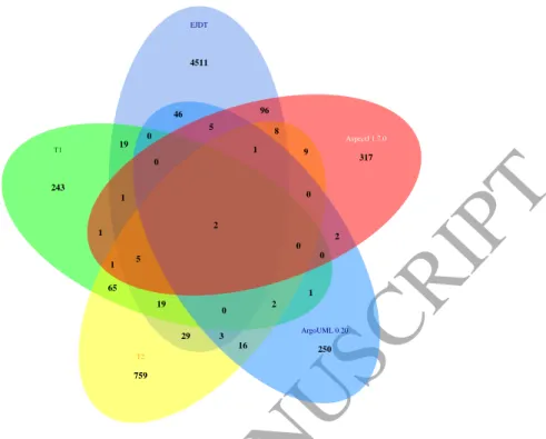
There are 6,411 AST n-grams11 significantly associated with faults in at least one of
the systems at the 99.9% level. Of these AST n-grams, 95% are significantly associated with faults in only one of the systems. The two commercial systems share around 7% of the same AST n-grams significantly associated with faults. Figure 5 shows that only two AST n-grams are significantly associated with faulty methods across all five systems. Had
the association been random we would have expected 0.03515×0.0196×0.0265×0.0036×
0.0027 = 0.00007219945 AST n-grams to be significantly associated with faults in all
sys-tems. The two AST n-grams which are significantly associated with faults in all five systems
11We refer to the number of AST n-gram types rather than the number of AST n-gram instances
ACCEPTED MANUSCRIPT
try {String n = bundle. g e t S t r i n g ( name [ i ]) ; if ( n != null && n . length () > 0) {
result [ i ] = n ; } else { result [ i ] = name [ i ]; } } catch ( M i s s i n g R e s o u r c e E x c e p t i o n e ) { result [ i ] = name [ i ]; }
Figure 4: The red portion of the text is the AST n-gram VARIABLE; MODIFIERS;
IDEN-TIFIER; METHOD INVOCATION; MEMBER SELECT; IDENTIFIER. MODIFIERS; IDENIDEN-TIFIER; METHOD INVOCATION MEMBER SELECT; IDENTIFIER; will be part of the same code, but does
not have theVARIABLEkind, which starts the line.
is greater than would be expected by chance (0.000312% > 0.00000000031%). These two
n-grams are: VARIABLE; MODIFIERS; IDENTIFIER; METHOD INVOCATION; MEMBER SELECT
IDENTIFIERandMODIFIERS; IDENTIFIER; METHOD INVOCATION; MEMBER SELECT; IDENTIFIER.
Example code of these AST grams is found in Figure 4, shown in red. Both of these n-grams are examples of a method call and are related to one another. This shows that methods with method calls could be more likely to be faulty across systems. Both of the n-grams have an odds ratio of 1.95, meaning that a method has nearly double chance of being faulty when it has a method call, compared to methods without a method call. Methods that do not contain method calls are less likely to be faulty across systems. This makes sense as these methods are likely to be methods such as getters, setters or interface methods and will be less fault prone.
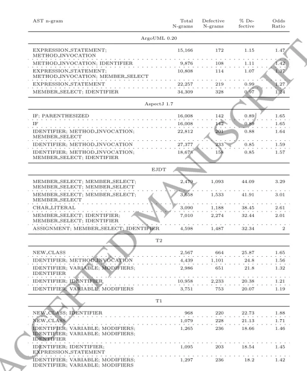
Table 8 shows that EJDT has the most AST n-grams significantly associated with faults (4,745) however, T2 has the largest by percentage (3.15%). ArgoUML has the least number of AST n-grams associated with faults (328). In EJDT more than 12% of the AST n-grams are significantly associated with faults. There does not seem to be a relationship between the number of unique AST n-grams and the number of AST n-grams that are significantly associated with faults.
System Unique AST n-grams Sig AST n-grams % T2 29,147 919 3.15 T1 18,351 359 1.96 EJDT 3.0 178,780 4,745 2.65 ArgoUML 90,499 328 0.36 AspectJ 165,005 448 0.27
Table 8: Table to show the total number of AST n-grams and AST n-grams significantly associated with
ACCEPTED MANUSCRIPT
4511 243 759 250 317 9 96 46 19 1 65 29 16 1 2 0 8 5 0 1 1 19 3 2 0 0 1 0 5 0 2 EJDT T1 T2 ArgoUML 0.20 AspectJ 1.7.0Figure 5: A Venn diagram to show the distribution of fault-prone AST n-grams between the systems. In total 2 AST n-grams are significantly associated with faults in all five systems.
Table 9 shows the top five most fault-prone AST n-grams in each system. Identifiers and
method calls appear often in the 25 AST n-grams shown. These n-grams includeIDENTIFIER
and METHOD INVOCATION. Some of these AST n-grams have very low odds-ratio, indicating
that they may not impact the overall faultiness of a method very much. However, some of
the ratios are still quite large. For example, IDENTIFIER METHOD INVOCATION has an odds
ratio of 1.56, meaning it could impact the faultiness of a method around 56% more than a method without this n-gram.
In each of the systems there are AST n-grams that are significantly associated with faults and that appear only in faulty methods. Table B.16 shows the n-grams which appear most often but only in faulty methods. All of the n-grams are around six or seven nodes in length, but appear infrequently. In the two commercial systems, the n-grams tend to appear around 20 times or less, in ArgoUML and AspectJ, the n-grams appear less than 10 times. This suggests possible differences between commercial and open source systems.
4.2. RQ2 - What is the effect size of AST n-grams significantly associated with faulty code?
A relatively high number of AST n-grams have a very large effect on the fault-proneness
of methods. For example, in EJDT the AST n-gramBREAK; CASE; INT LITERAL;
EXPRESSION STATEMENT; METHOD INVOCATION; IDENTIFIER appears only in faulty
meth-ods, so will have an odds-ratio of infinity. This AST n-gram will be linked to a piece of code in a switch statement. Over 1,000 other AST n-grams appear only in faulty methods in EJDT. Most of these exclusively faulty AST n-grams occur infrequently with those in EJDT appearing on average around 15 times. The same phenomenon is also present in
ACCEPTED MANUSCRIPT
AST n-gram Total
N-grams Faulty N-grams % Faulty Odds-Ratio T2 3.15 IDENTIFIER 39,371 7,361 18.70 1.09 IDENTIFIER; IDENTIFIER 10,958 2,233 20.38 1.21
IDENTIFIER; METHOD INVOCATION 4,439 1,101 24.80 1.56
VARIABLE; MODIFIERS; IDENTIFIER 5,296 1,057 19.96 1.18
METHOD INVOCATION; IDENTIFIER 4,676 915 19.57 1.15
T1 1.96
IDENTIFIER; IDENTIFIER 6,541 991 15.15 1.14
IDENTIFIER; IDENTIFIER; IDENTIFIER 1,762 298 16.91 1.30
IDENTIFIER; METHOD INVOCATION; MEMBER SELECT; IDENTIFIER
1,758 293 16.67 1.27
IDENTIFIER; EXPRESSION STATEMENT; 1,531 275 17.96 1.40
IDENTIFIER; VARIABLE; MODIFIERS; IDENTIFIER; VARIABLE; MODIFIERS; IDENTIFIER
1,265 236 18.66 1.46
EJDT 3.0 2.65
MEMBER SELECT 90,007 21,440 23.82 1.31
MEMBER SELECT; IDENTIFIER 71,051 16,267 22.89 1.24
EXPRESSION STATEMENT 38,603 7,816 20.25 1.06
PARENTHESIZED 29,105 6,403 22.00 1.18
IF; PARENTHESIZED 19,325 4,390 22.72 1.23
ArgoUML 0.20 0.36
METHOD INVOCATION 54,926 505 0.92 1.19
MEMBER SELECT; IDENTIFIER 34,309 328 0.96 1.24
EXPRESSION STATEMENT 22,257 219 0.98 1.27
EXPRESSION STATEMENT; METHOD INVOCATION 15,166 172 1.13 1.47 EXPRESSION STATEMENT; METHOD INVOCATION;
MEMBER SELECT
10,808 114 1.05 1.37
AspectJ 1.7.0 0.27
MEMBER SELECT 92,366 630 0.68 1.27
METHOD INVOCATION 83,991 550 0.65 1.22
MEMBER SELECT; IDENTIFIER 73,475 527 0.72 1.34
METHOD INVOCATION; MEMBER SELECT 64,647 492 0.76 1.42
METHOD INVOCATION; MEMBER SELECT; IDENTIFIER 51,380 395 0.77 1.43
ACCEPTED MANUSCRIPT
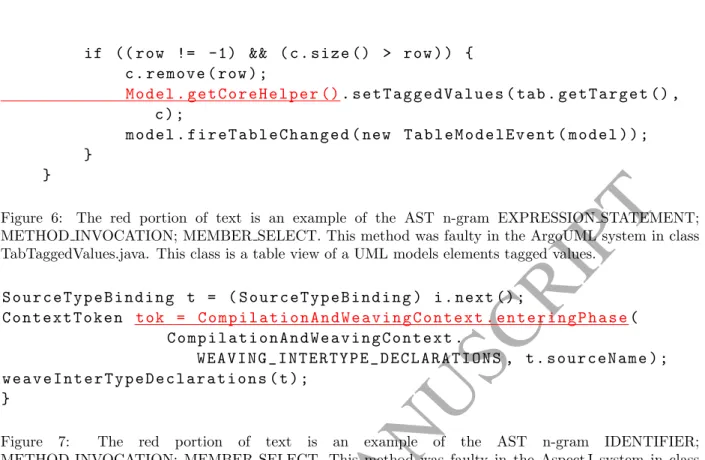
if (( row != -1) && ( c . size () > row ) ) {c . remove ( row ) ;
Model . g e t C o r e H e l p e r (). s e t T a g g e d V a l u e s ( tab . g e t T a r g e t () , c ) ;
model . f i r e T a b l e C h a n g e d ( new T a b l e M o d e l E v e n t ( model ) ) ; }
}
Figure 6: The red portion of text is an example of the AST n-gram EXPRESSION STATEMENT; METHOD INVOCATION; MEMBER SELECT. This method was faulty in the ArgoUML system in class TabTaggedValues.java. This class is a table view of a UML models elements tagged values.
S o u r c e T y p e B i n d i n g t = ( S o u r c e T y p e B i n d i n g ) i . next () ; C o n t e x t T o k e n tok = C o m p i l a t i o n A n d W e a v i n g C o n t e x t . e n t e r i n g P h a s e( C o m p i l a t i o n A n d W e a v i n g C o n t e x t . W E A V I N G _ I N T E R T Y P E _ D E C L A R A T I O N S , t . s o u r c e N a m e ) ; w e a v e I n t e r T y p e D e c l a r a t i o n s ( t ) ; }
Figure 7: The red portion of text is an example of the AST n-gram IDENTIFIER;
METHOD INVOCATION; MEMBER SELECT. This method was faulty in the AspectJ system in class AjLookupEnvironment. This class overrides the default EJDT LookupEnvironment.
ArgoUML, AspectJ and the two commercial systems. In these systems the mean number of times an exclusively faulty n-gram occurs is lower than EJDT at around 5, 2, 6 and 7 respectfully. Such infrequently occurring fault-prone AST n-grams contribute relatively little to the overall faultiness of a system.
However, many AST n-grams with a relatively large effect on fault-proneness do appear more frequently. Such AST n-grams are likely to have more impact on the overall faultiness of a system. Table 10 show fault-prone AST n-grams that appear more than two standard deviations away from the mean number of faulty n-grams in all five of the systems studied in this paper. For example, those n-grams chosen for EJDT will be only those n-grams which
have over 1,032 faulty n-grams (84.43 + (2×473.91)). These n-grams will have a greater
impact on the overall faultiness of a system.
Figures 8, 6 and 7 show source code examples of AST n-grams with the highest effect size for the open source systems. The underlined red text highlights which source code is covered by the AST n-gram. The methods that have been chosen for these code examples
are methods that have been identified as faulty12. Figure 9 shows an example method from
EJDT to highlight the AST n-gram with the largest effect size for each of the commercial telecommunications systems. We are unable to publish source code from these systems for commercial reasons.
12It is important to note that the red text that is highlighted may not be the cause of the fault in the
ACCEPTED MANUSCRIPT
AST n-gram Total
N-grams Defective N-grams % De-fective Odds Ratio ArgoUML 0.20 EXPRESSION STATEMENT; METHOD INVOCATION 15,166 172 1.15 1.47
METHOD INVOCATION; IDENTIFIER 9,876 108 1.11 1.42 EXPRESSION STATEMENT;
METHOD INVOCATION; MEMBER SELECT
10,808 114 1.07 1.37
EXPRESSION STATEMENT 22,257 219 0.99 1.27
MEMBER SELECT; IDENTIFIER 34,309 328 0.97 1.24
AspectJ 1.7
IF; PARENTHESIZED 16,008 142 0.89 1.65
IF 16,008 142 0.89 1.65
IDENTIFIER; METHOD INVOCATION; MEMBER SELECT
22,812 201 0.88 1.64
IDENTIFIER; METHOD INVOCATION 27,377 233 0.85 1.59 IDENTIFIER; METHOD INVOCATION;
MEMBER SELECT; IDENTIFIER
18,678 158 0.85 1.57
EJDT MEMBER SELECT; MEMBER SELECT;
MEMBER SELECT; MEMBER SELECT
2,479 1,093 44.09 3.29 MEMBER SELECT; MEMBER SELECT;
MEMBER SELECT
3,658 1,533 41.91 3.01
CHAR LITERAL 3,090 1,188 38.45 2.61
MEMBER SELECT; IDENTIFIER; MEMBER SELECT; IDENTIFIER
7,010 2,274 32.44 2.01 ASSIGNMENT; MEMBER SELECT; IDENTIFIER 4,598 1,487 32.34 2
T2
NEW CLASS 2,567 664 25.87 1.65
IDENTIFIER; METHOD INVOCATION 4,439 1,101 24.8 1.56 IDENTIFIER; VARIABLE; MODIFIERS;
IDENTIFIER
2,986 651 21.8 1.32
IDENTIFIER; IDENTIFIER 10,958 2,233 20.38 1.21
IDENTIFIER; VARIABLE; MODIFIERS 3,751 753 20.07 1.19 T1
NEW CLASS; IDENTIFIER 968 220 22.73 1.88
NEW CLASS 1,079 228 21.13 1.71
IDENTIFIER; VARIABLE; MODIFIERS; IDENTIFIER; VARIABLE; MODIFIERS; IDENTIFIER
1,265 236 18.66 1.46
IDENTIFIER; IDENTIFIER; EXPRESSION STATEMENT
1,095 203 18.54 1.45
IDENTIFIER; VARIABLE; MODIFIERS; IDENTIFIER; VARIABLE; MODIFIERS
1,297 236 18.2 1.42
Table 10: Table to show the AST n-grams with the greatest odds ratios and also appear in over two standard deviations from the mean in all five systems.
ACCEPTED MANUSCRIPT
this . c o n t e n t s [ l o c a l C o n t e n t s O f f s e t ++] = ( byte ) n a m e I n d e x ; d e s c r i p t o r I n d e x = c o n s t a n t P o o l . l i t e r a l I n d e x ( c o d e S t r e a m . m e t h o d D e c l a r a t i o n . binding . d e c l a r i n g C l a s s . s i g n a t u r e() ) ; this . c o n t e n t s [ l o c a l C o n t e n t s O f f s e t ++] = ( byte ) ( d e s c r i p t o r I n d e x >> 8) ;Figure 8: The red portion of text is an example of the AST n-gram MEMBER SELECT;
MEM-BER SELECT; MEMMEM-BER SELECT; MEMMEM-BER SELECT. This is a part of a longer method that was faulty in the EJDT 3.0 system in class ClassFile.java. This class represents a class file wrapper on bytes.
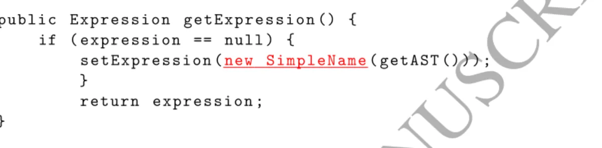
public E x p r e s s i o n g e t E x p r e s s i o n () { if ( e x p r e s s i o n == null ) { s e t E x p r e s s i o n (new S i m p l e N a m e( getAST () ) ) ; } return e x p r e s s i o n ; }
Figure 9: The red portion of text is an example of the AST n-gram NEW CLASS; IDENTIFIER which has the largest effect size for T2 and T1. This method was taken from a method in EJDT 3.0. We are unable to show code from the T2 or the T1 system.
Figure 8 highlights an example of AST n-gram with the highest effect size in EJDT. This n-gram is a long message chain, with four different object requests. In this case too, the result of this long message chain has been used as a variable in a method call. Long message chains have been identified in the past as a problem [25, 32]. Figures 6 and 7 also show examples of message chains as these AST n-grams had the highest effect sizes for these two systems.
4.3. RQ3: Does the inclusion of AST n-grams significantly associated with faults in software defect prediction models help improve their predictive performance?
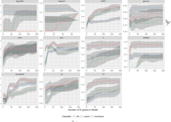
Yes. The inclusion of AST n-grams significantly associated with faults can result in sig-nificant improvements on a models predictive performance. In some cases, these increases are very large. Figure 10 shows how MCC performance changes as AST n-grams significantly
associated with faults are added to the 11 systems studied13. In all 11 systems MCC has
improved due to the inclusion of AST n-grams and in nine of the 11 systems, these improve-ments are seen across all three classifiers. The biggest increase in median MCC performance can be seen in EJDT, where J48 has risen by around 0.39, from 0.19 to around 0.58 (213%). In percentage terms, the biggest median increase was in T1 using logistic regression, where MCC increased by just over 3,900% (0.0007 to 0.27) from the baseline model. The biggest increase over all performance measures was seen in Reddeer, where the median precision of
ACCEPTED MANUSCRIPT
the logistic regression model median went from 0 to 0.52 (a percentage increase could not be calculated). The biggest median percentage increase across all performance measures was for the recall in T1 using logistic regression. The median increased by just below 12,000% (0.002 to 0.22).
SocialSDK T1 T2
jmol jmri k reddeer
ArgoUML AspectJ EJDT genoviz
0 50 100 150 200 0 50 100 150 200 0 50 100 150 200 0 50 100 150 200 0 50 100 150 200 0 50 100 150 200 0 50 100 150 200 0 50 100 150 200 0 20 40 60 0 50 100 150 200 0 50 100 150 200 0.10 0.15 0.20 0.25 0.30 0.0 0.1 0.2 0.3 0.4 0.2 0.3 0.4 0.5 0.6 0.0 0.1 0.2 0.3 0.4 0.2 0.3 0.4 0.5 0.0 0.1 0.2 0.3 0.2 0.3 0.4 0.5 0.0 0.1 0.2 0.3 0.00 0.05 0.10 0.15 0.20 0.1 0.2 0.3 0.4 0.0 0.1 0.2 0.3 0.4
Number of N−grams in Model
Median MCC
Classifier J48 Logistic NaiveBayes
Figure 10: A line plot to show the change in MCC across all the 11 systems when different levels of N-grams are added to the baseline models.
In the majority of cases, MCC increases as a greater number of AST n-grams are added. For example, in EJDT, the addition of 10 AST n-grams significantly associated with faults significantly improves the MCC median from 0.19, when using no AST n-grams, to 0.37 (a
97% increase)14. When 20 AST n-grams are added, the MCC median increases again by
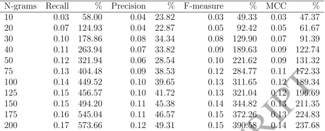
around 0.1 (3%), these increases continue and when 200 AST n-grams significantly associated with faults are added, the median MCC has risen just over 212% (0.40) on the original baseline model MCC median (0.19). Table 11 shows that on average over all the systems, adding 10 AST n-grams improves MCC by around 47%, 50 n-grams by around 131% and 200 n-grams 238%. These improvements are also seen in recall (58%, 322% and 574%), precision (24%, 29% and 49%) and f-measure (49%, 222% and 391%).
Despite the poor performance of the models in some of the systems, most notably Ar-goUML and AspectJ, AST n-grams can make a significant impact. For example, there is an increase with ArgoUML and Logistic, where MCC raises from around 0.03 to around 0.10 when 75 AST n-grams are added, then stays steady until 200. This could suggest that there was an AST n-gram that has a large effect added in the 50-75 bracket. Similarity, systems
ACCEPTED MANUSCRIPT
N-grams Recall % Precision % F-measure % MCC %
10 0.03 58.00 0.04 23.82 0.03 49.33 0.03 47.37 20 0.07 124.93 0.04 22.87 0.05 92.42 0.05 61.67 30 0.10 178.86 0.08 34.34 0.08 129.90 0.07 91.39 40 0.11 263.94 0.07 33.82 0.09 189.63 0.09 122.74 50 0.12 321.94 0.06 28.54 0.10 221.62 0.09 131.32 75 0.13 404.48 0.09 38.53 0.12 284.77 0.11 172.33 100 0.14 449.52 0.10 39.65 0.13 311.65 0.12 189.34 125 0.15 456.57 0.10 41.72 0.13 321.04 0.12 196.69 150 0.15 494.20 0.11 45.38 0.14 344.82 0.13 211.35 175 0.16 545.04 0.11 46.57 0.15 372.26 0.13 224.83 200 0.17 573.66 0.12 49.31 0.15 390.58 0.14 237.68
Table 11: Average changes in the performance measures when AST n-grams significantly associated with defects are added to the base line models
K, Reddeer, SocialSDK and T1 have an MCC which is around 0 using the baseline metrics and the Logistic model. The inclusion of n-grams, allows the logistic models performance increase to around 0.20. AspectJ with J48 sees an increase in MCC from 0 to around 0.20 by the time 75 AST n-grams have been added. AspectJ had on average only 69 significant n-grams in each run and fold, so we were unable to get results beyond a maximum of 75 n-grams for this system. The poor performance of AspectJ and ArgoUML is probably due to the very low proportion of defective methods (see Table 3) in the systems, which is a known problem [3].
Figure 12 plots the median effect size of the change between the defect prediction perfor-mance measure MCC with no n-grams and the different numbers of significant AST n-grams. The highest effect sizes are found in EJDT, JMRI and SocialSDK, where Cliff’s D reacts the maximum 1. In JMOL it reaches this maximum after 30 AST n-grams using both Naive Bayes and logistic regression. Generally, the more AST n-grams that are added to the model, the greater the effect on the models. In all of the systems, the AST n-grams have eventually a large effect on at least one of the classifiers. In six of the systems, the AST n-grams have a large effect on all of the classifiers. The AST n-grams have at least a small effect on MCC in all of the classifiers in nine of the 11 systems, AspectJ and ArgoUML being the only
two systems to miss out. Similar effect sizes are seen for the other performance measures15.
Table 12 shows that at the when 200 AST n-grams significantly associated with faults are added to the models, the performance measure they have the most effect on is recall, with an average median effect size of 0.80, whilst the lowest effect is on precision, with an average median effect size of 0.43. If we look at all the different n-gram levels, then recall is still has the largest average effect sizes with a Cliffs D value of 0.56, whilst AST n-grams only have a small effect on the precision (0.25). 200 AST n-grams have the largest effect on the logistic classifier performance, with an average effect size of around 0.80. Naive Bayes and J48 have an average large effect size of 0.66 and 0.57 respectfully when 200 AST n-grams are added.
ACCEPTED MANUSCRIPT
Over all the AST n-grams, the average median effect sizes for the classifiers come down to 0.51, 0.45 and 0.40 respectfully, which is around the large effect threshold.
SocialSDK T1 T2
jmol jmri k reddeer
ArgoUML AspectJ EJDT genoviz
0 50 100 150 0 10 20 30 40 50 0 20 40 60 0 10 20 30 40 50 0 50 100 150 200 0 10 20 30 40 50 0 5 10 15 20 0 10 20 30 40 0 20 40 60 0 10 20 30 40 50 0 25 50 75 100 0.15 0.20 0.25 0.30 0.0 0.1 0.2 0.3 0.15 0.20 0.25 0.30 0.0 0.1 0.2 0.3 0.4 0.2 0.3 0.4 0.0 0.1 0.2 0.0 0.1 0.2 0.3 0.00 0.05 0.10 0.15 0.20 0.25 0.00 0.05 0.10 0.15 0.20 0.0 0.1 0.2 0.3 0.00 0.05 0.10 0.15 0.20
Number of N−grams in Model
Median MCC
Classifier J48 Logistic NaiveBayes
Figure 11: A line plot to show the change in MCC across all the 11 systems when different levels of N-grams are added to the baseline models when using the reduced Wang et al. [71] AST node set.
Measure J48 Logistic Naive Bayes All
Recall 0.6450 0.8975 0.8492 0.7973
Precision 0.3373 0.6115 0.3483 0.4324
F-measure 0.6678 0.8862 0.7347 0.7629
MCC 0.6267 0.8118 0.6952 0.7112
Table 12: The average Cliff’s D effect score for all the systems when 200 AST n-grams significantly associated
with faults are added to the base line models (d<0.147 Negligible, d<0.33 = small, d<0.474 = medium,
d>0.474 large [59])
4.3.1. Comparing the performance of the full set to Wang et al. [71] reduced set
Figure 11 shows that using the reduced set that Wang et al. [71] proposed does not achieve the same results as the full set. Firstly, for most of the systems, the number of AST n-grams found in the systems is lower than that for models built with the full set of available nodes. In most cases, the median MCC performance across systems does not rise as dramatically as with the full available AST nodes, or does not rise at all. For example, J48’s median MCC in EJDT only rises around 0.04 from the baseline of 0.19 to a 50 AST n-grams MCC of 0.23. This 22% rise is significant (at the 99% level), however this has only
ACCEPTED MANUSCRIPT
k reddeer SocialSDK
ArgoUML genoviz jmol jmri
EJDT T1 T2 AspectJ 10 20 30 40 50 75 100 125 150 175 200 10 20 30 40 50 75 100 125 150 175 200 10 20 30 40 50 75 100 125 150 175 200 10 20 30 40 50 75 100 125 150 175 200 10 20 30 40 50 75 100 125 150 175 200 10 20 30 40 50 75 100 125 150 175 200 10 20 30 40 50 75 100 125 150 175 200 10 20 30 40 50 75 100 125 150 175 200 10 20 30 40 50 75 100 125 150 175 200 10 20 30 40 50 75 100 125 150 175 200 10 20 30 40 50 75 −0.5 0.0 0.5 1.0 −0.5 0.0 0.5 1.0 −0.5 0.0 0.5 1.0 AST n−grams Median Eff ect Siz e (using Cliffs D)
Classifier J48 Logistic NaiveBayes
Figure 12: A line plot to show the level of effect on the performance measure MCC when AST n-grams are
added to our models. The three grey straight lines are the effect size indicators (d<0.147 Negligible, d<0.33
ACCEPTED MANUSCRIPT
a small effect size (0.31). This rise is 0.26 (114%) less than what is achieved using the full sets 50 AST n-grams significantly associated with faults and 0.35 less (156%) less than the full sets 200 AST n-grams (both significant at the 99% level). Overall, median MCC is 0.07 (38%) higher using the full set, compared the Wang et al. [71] reduced set across all the systems and classifiers. Recall is on average 0.08 (45%) higher using the full set, precision
0.08 (22%) higher and f-measure 0.08 (39%) higher. Table 13 shows the difference16 in
performance measures across all of the AST n-gram levels. MCC and recall perform much better in the full set of AST nodes, by performing on average up to 472% and 279% better than the reduced set respectfully. On average, precision is less impacted by the reduction of the AST nodes, where there is minimal difference in the performance of our models built with the two different AST node sets between 0-50 n-grams and then an increase of up to 64% between 50 and 150 AST n-grams significantly associated with faults.
Recall Precision F-measure MCC
N-grams Change % Change % Change % Change %
10 0.01 0.00 0.02 0.00 0.02 0.00 0.02 6.62 20 0.02 4.82 0.02 0.00 0.02 5.32 0.03 12.55 30 0.04 20.68 0.03 1.59 0.05 14.17 0.05 21.04 40 0.06 45.80 0.02 0.00 0.06 16.58 0.05 34.24 50 0.10 69.96 -0.00 -0.47 0.07 25.85 0.07 35.20 75 0.08 22.71 0.07 2.76 0.10 18.32 0.10 33.58 100 0.09 194.72 0.05 11.11 0.08 159.20 0.08 91.31 125 0.22 452.86 0.16 66.44 0.27 323.81 0.23 223.04 150 0.20 472.41 0.14 64.02 0.26 259.29 0.20 279.47
Table 13: Median changes between the models built using the full set of AST nodes vs the reduced Wang et al. [71] set (Full set - reduced set).
Figure 13 shows a line plot of the effect of reducing the number of available AST nodes on the performance measure MCC across the systems, where a score of 1 means that the full set is performing better than the reduced set, 0 there is no effect of using the full set or the reduced set and -1 means the reduced set is performing better than the full set. The effect of using the full set over the reduced set is normally greater. In EJDT, T2, AspectJ and SocialSDK for all classifiers the effect on the performance of MCC when using the full set of AST nodes is very large compared to using the reduced set. In some instances, the there is a small effect in the favour of using the reduced set. For example, in GenoViz, logistic regression never goes above zero and stays at an average of -0.15. Overall, the effect on the performance of the model is greater if we use the full set compared to the reduced. Table 14 shows the median effect sizes over the 11 systems for each of the four effect sizes and classifiers. There is on average, a large effect on the change in recall (0.67) and f-measure (0.51), a medium effect on the change in MCC (0.41) and a negligible effect in the change in precision (0.12).
ACCEPTED MANUSCRIPT
k reddeer SocialSDK
ArgoUML genoviz jmol jmri
EJDT T1 T2 AspectJ 10 20 30 40 50 10 20 10 20 30 40 50 75100 125 150 10 20 30 40 10 20 30 40 50 75 100 10 20 30 40 50 10 20 30 40 50 75 100 125 150 175 200 10 20 30 40 50 10 20 30 40 50 10 20 30 40 50 75 10 20 30 40 50 75 −0.5 0.0 0.5 1.0 −0.5 0.0 0.5 1.0 −0.5 0.0 0.5 1.0 AST n−grams Median Eff ect Siz e (using Cliffs D)
Classifier J48 Logistic NaiveBayes
Figure 13: A line plot to show the level of effect on the change of the performance measure MCC between the full AST node set vs Wang et al. [71]’s reduced set. The three grey straight lines are the effect size
ACCEPTED MANUSCRIPT
column J48 Logistic Naive Bayes All
Recall 0.4874 0.6533 0.8727 0.6711
Precision 0.1748 0.0891 0.1016 0.1218
F-measure 0.5141 0.5646 0.4461 0.5082
MCC 0.4948 0.3187 0.4103 0.4080
Table 14: The average Cliff’s D effect score for all the systems between the changes in using the full set
and Wang et al. [71]’s reduced set of AST nodes (d<0.147 Negligible, d<0.33 = small, d<0.474 = medium,
d>0.474 large [59])
5. Threats to Validity
There are threats to validity in the research presented in this paper which fall into the categories of internal, external and construct validity.
5.1. Internal Validity
An internal threat is the small number of faults reported for both ArgoUML and AspectJ. These small datasets create the problem that it may be difficult to generate statistically significant results. It is always difficult to generate significant results with small sets of data. A small number of faults is typical of many software systems and we feel it is a particular strength that our technique is able to find significant results in the systems despite a small number of faults. The technique we show does find significant results and also finds some of the same significant AST n-grams as those found in the systems with larger numbers of reported faults.
The processing power available to us meant that we had to limit the maximum length of an AST n-gram. Limiting the length of an AST n-gram to seven means that we have not investigated possible significant AST n-grams that are over this length. There could be frequently occurring longer significant AST n-grams that are significantly associated with faulty code. With greater processing power, longer AST n-grams could be analysed.
The statistical evaluations used could be a threat to the results published in this paper. We have used significance testing which has its critics [20]. We have tried to alleviate the problems that occur with statistical testing by having a large alpha value (0.001) and by using non-parametric tests. Also, we do not say that the AST n-grams are definitely associated with faults, just that there is evidence to suggest that the faulty AST n-grams appear in a greater number of faults than that could be given by chance. There could be some AST n-grams that have been designated as significantly associated with faults that do not have an overall effect. We have tried to overcome this threat by including the effect sizes of all the AST n-grams with sufficient evidence to reject our null hypothesis. We do not assume that the AST n-gram is the root cause of any fault that has occurred in any of the systems, just that they appear to be in a higher number of faulty methods than could have happened by chance.
We have not controlled for programming confounds which result in different AST n-grams being extracted from the source code. For example, we have not controlled for the developer experience of the developers from either the open source or commercial projects
ACCEPTED MANUSCRIPT
or the coding guidelines put in place by the company. At the communications company, there is a guideline that all methods and classes must be kept as short as possible, this could have impacted on the number of n-grams we could have extracted from their code.
5.2. External Validity
An external threat is the number of systems chosen to analyse. The technique shown in this paper may only work for these systems and may not translate to smaller or larger systems. Our technique works on systems with a high or low number of identified faults and both commercial and open source systems. We have shown that the AST n-grams signifi-cantly associated with faults in all of the systems can have an impact on the performance of defect prediction models. The technique itself could be easily applied to other Java systems. The commercial systems may not be representative to other open source or commercial sys-tems, however it is very difficult to analyse this as it is extremely difficult to gain access to commercial fault data.
Another external threat is that we have only extracted AST n-grams from the Java programming language. We have not extracted code constructs from other programming languages such as C/C++ or Python. There may not be AST n-grams significantly associ-ated with faults nor might they help improve software defect prediction performance when added to the baseline models in these languages. The technique could be applied to other programming languages with the use of specific AST parsers and this is future work.
5.3. Construct Validity
Repository mining to find faulty code in systems is an inexact science. Latent defects may not have been discovered and may lie dormant in the code base. Faults may also have been fixed but not reported properly in t