Progressive Indexes:
Indexing for Interactive Data Analysis
Pedro Holanda
CWI, AmsterdamMark Raasveldt
CWI, AmsterdamStefan Manegold
CWI, AmsterdamHannes M ¨uhleisen
CWI, AmsterdamABSTRACT
Interactive exploration of large volumes of data is increasingly common, as data scientists attempt to extract interesting in-formation from large opaque data sets. This scenario presents a difficult challenge for traditional database systems, as (1) nothing is known about the query workload in advance, (2) the query workload is constantly changing, and (3) the sys-tem must provide interactive responses to the issued queries. This environment is challenging for index creation, as tra-ditional database indexes require upfront creation, hence a priori workload knowledge, to be efficient.
In this paper, we introduceProgressive Indexing, a novel performance-driven indexing technique that focuses on au-tomatic index creation while providing interactive response times to incoming queries. Its design allows queries to have a limited budget to spend on index creation. The indexing budget is automatically tuned to each query before query processing. This allows for systems to provide interactive answers to queries during index creation while being robust against various workload patterns and data distributions.
PVLDB Reference Format:
Pedro Holanda, Mark Raasveldt, Stefan Manegold and Hannes M¨uhleisen. Progressive Indexes: Indexing for Interactive Data Analysis. PVLDB, 12(13): 2366-2378, 2019.
DOI: https://doi.org/10.14778/3358701.3358705
1.
INTRODUCTION
Data scientists perform exploratory data analysis to dis-cover unexpected patterns in large collections of data. This process is done with a hypothesis-driven trial-and-error ap-proach [26]. They query segments that could potentially provide insights, test their hypothesis, and either zoom in on the same segment or move to a different one depending on the insights gained.
Fast responses to queries are crucial to allow for interactive data exploration. The study by Liu et al. [18] shows that any delay larger than 500ms (the “interactivity threshold”) sig-nificantly reduces the rate at which users make observations
This work is licensed under the Creative Commons Attribution-NonCommercial-NoDerivatives 4.0 International License. To view a copy of this license, visit http://creativecommons.org/licenses/by-nc-nd/4.0/. For any use beyond those covered by this license, obtain permission by emailing [email protected]. Copyright is held by the owner/author(s). Publication rights licensed to the VLDB Endowment.
Proceedings of the VLDB Endowment,Vol. 12, No. 13 ISSN 2150-8097.
DOI: https://doi.org/10.14778/3358701.3358705
and generate hypotheses. When dealing with small data sets, providing answers within this interactivity threshold is possible without utilizing indexes. However, exploratory data analysis is often performed on larger data sets as well. In these scenarios, indexes are required to speed up query response times.
Index creation is one of the major difficult decisions in database schema design [8]. Based on the expected work-load, the database administrator (DBA) needs to decide whether creating a specific index is worth the overhead in creating and maintaining it. Creating indexes up-front is especially challenging in exploratory and interactive data analysis, where queries are not known in advance, workload patterns change frequently and interactive responses are re-quired. In these scenarios, data scientists load their data and immediately want to start querying it without waiting for index construction. In addition, it is also not certain whether or not creating an index is worth the investment at all. We cannot be sure that the column will be queried frequently enough for the large initial investment of creating a full index to pay off.
In spite of these challenges, indexing remains crucial for im-proving database performance. When no indexes are present, even simple point and range selections require expensive full table scans. When these operations are performed on large data sets, indexes are essential to ensure interactive query response times. There are two main strategies that aim to release the DBA of having to manually choose which indexes to create.
(1) Automated index selection techniques [1, 7, 30, 10, 6, 4, 19, 27] accomplish this by attempting to find the optimal set of indexes given a query workload, taking into account the benefits of having an index versus the added costs of creating the entire index and maintaining it during modifications to the database. However, these techniques require a priori knowledge of the expected workloads and do not work well when the workload is not known or changes frequently. Hence they are not suitable for interactive data exploration.
(2) Adaptive indexing techniques such as database crack-ing [16, 9, 24, 23, 12, 15, 17, 21, 20, 11, 14, 13] are a more promising solution. They focus on automatically and incre-mentally building an index as a side effect of querying the data. An index for a column is only initiated when it is first queried. As the column is queried more, the index is refined until it eventually approaches the performance of a full index. In this way, the cost of creating an index is smeared out over the cost of querying the data many times, though not necessarily equally, and there is a smaller initial overhead
for starting the index creation. However, since the index is refined only in the areas targeted by the workload, conver-gence to a full index is not guaranteed and partitions can have different sizes. The performance of the query degrades when a less refined part of the index is queried, resulting in performance spikes whenever the workload changes.
In this paper, we introduce a new incremental indexing technique calledProgressive Indexing. It differs from other in-dexing solutions in that the inin-dexing budget (i.e., the amount of time that is spent on index creation and refinement) can be controlled. We provide two indexing budget flavors: a fixed indexing budget, where the user defines a fixed amount of time to spend on indexing per query, and an adaptive index-ing budget, where the indexindex-ing budget is adapted so that the total time spent on query execution remains constant. As a result, Progressive Indexing complements existing automatic indexing techniques by offering predictable performance and deterministic convergence independent of the workload.
The main contributions of this paper are:
• We introduce several novel Progressive Indexing tech-niques and investigate their performance, convergence, and robustness in the face of various realistic synthetic workload patterns and real-life workloads.
• We provide a cost-model for each of the Progressive Indexing techniques. The cost models are used to automatically adapt the indexing budget.
• We experimentally verify that the Progressive Indexing techniques we propose provide robust and predictable performance and convergence regardless of the work-load or data distribution.
• We provide a decision tree to assist in choosing an indexing technique for a given scenario.
• We provide Open-Source implementations of each of the techniques we describe and their benchmarks.1
Outline. This paper is organized as follows. In Section 2,
we investigate related research that has been performed on automatic/adaptive index creation. In Section 3, we describe our novel Progressive Indexing techniques and discuss their benefits and drawbacks. In Section 4, we perform an experi-mental evaluation of each of the novel methods we introduce, and we compare them against adaptive indexing techniques. In Section 5 we draw our conclusions and present a deci-sion tree to assist in choosing which Progressive Indexing technique to use. Finally, in Section 6 we discuss future work.
2.
RELATED WORK
Automatic index creation and maintenance has been a challenging and long-standing problem in database research. Even when the workload pattern is known, selecting the optimal set of indexes is an NP-Hard problem [8]. When the querying pattern is not known in advance, optimal a-priori index creation is impossible. Automatic indexing techniques can be grouped into two categories, (1) automatic index selection and (2) adaptive index creation.
1Our implementations and benchmarks are available at
https://github.com/pdet/ProgressiveIndexing
2.1
Automatic Index Selection
Automatic index selection techniques [1, 7, 30, 10, 6, 19, 27, 4] attempt to solve the problem by, given an existing (or expected) workload of the system, selecting the set of indexes that would result in optimal performance. The problem with these methods is that they can only be used when the workload of the system is known and stable. In an environment where the workload is unknown or rapidly changing, beyond what is known upfront, automatic index selection techniques do not offer much help. In addition, these techniques require sufficient time and space to invest in constructing a large full index upfront.
2.2
Adaptive Indexing
Adaptive indexing techniques are an alternative to a priori index creation. Instead of constructing the index upfront, the index is constructed as a by-product of querying the data. These techniques are designed for scenarios where the workload is unknown, and there is no idle time to invest in index creation. The high investment of creating an up-front full index is smeared out over the cost of subsequent queries. Database Cracking [16] (also known as “Standard Crack-ing”) is the original adaptive indexing technique. It works by physically reordering the index while processing queries. It consists of two data structures: a cracker column and a cracker index. Each incoming query cracks the column into smaller pieces and then updates the cracker index with the reference to those pieces. As more queries are processed, the cracker index converges towards a full index.
While database cracking accomplishes its mission of con-structing an index as a by-product of querying, it suffers from several problems that make it unsuitable for interactive data analysis: (1) cracking adds a significant overhead over naive scans in the first iterations of the algorithm, (2) the performance of cracking is not robust, as sudden changes in workload cause spikes in performance, and (3) convergence towards a full index is slow and workload-dependent.
There is a large body of work on extending and improv-ing database crackimprov-ing. These improvements include better convergence towards a full index [9, 24], more predictable per-formance [23, 12], more efficient tuple reconstruction [15, 17, 24], better CPU utilization [20], other cracking engines [21, 11], predictive query processing [29] and handling updates [14, 13]. Below, we give an overview of the work done on improv-ing robustness and general performance.
Cracking Kernels[21, 11] addresses the low CPU
effi-ciency caused by the high number of branch mispredictions. It suggests different cracking kernels that reorganize the ele-ments by exploiting either predication, vectorization, SIMD instructions, or memory rewiring. Haffner et al. [11] present a decision tree that recommends the most efficient cracking kernel depending on the query selectivity, type size, and data organization.
Stochastic Cracking [12] addresses the unpredictable
performance problem by creating partitions using a random pivot element instead of pivoting around the query predicates. The pivot is used to perform arbitrary reorganization steps for more robust query performance.
Progressive Stochastic Cracking[12] performs
stochas-tic cracking in a partial fashion every iteration. It takes two input parameters, the size of the L2 cache and the number of swaps allowed in one iteration (i.e., a percentage of the total column size). When performing stochastic cracking,
progressive stochastic cracking will only perform at most the maximum allowed number of swaps on pieces larger than the L2 cache. If the piece fits into the L2 cache, it will always perform a complete crack of the piece.
Coarse-Granular Index[24] improves stochastic
crack-ing robustness by creatcrack-ing equal-sized partitions when the first query is executed. It also allows for the creation of any number of partitions instead of limiting the number of parti-tions to two, letting the DBA decide between the trade-off of the higher cost of the first query versus building a more robust index.
Adaptive Adaptive Indexing [23] is a general-purpose
algorithm for adaptive indexing. It has multiple parameters that can be tuned to mimic the data access of different adap-tive indexing techniques (e.g., database cracking, sideways cracking, hybrid cracking). It also uses radix partitioning and exploits software managed buffers using nontemporal streaming stores to achieve better performance [25].
3.
PROGRESSIVE INDEXING
In this section, we introduce Progressive Indexing. The core features of Progressive Indexing are that (1) the indexing overhead per query is controllable, both in terms of time and memory requirements, (2) it offers robust performance and deterministic convergence regardless of the underlying data distribution, workload patterns or query selectivity, and (3) the indexing budget can be automatically tuned so more expensive queries spend less extra time on indexing while cheaper queries spend more.
As a result of the small initial cost, Progressive Indexing occurs without significantly impacting worst-case query per-formance. Even if the column is only queried once, only a small penalty is incurred. On the other hand, if the column is queried hundreds of times, the index will reliably converge towards a full index and queries will be answered at the same speed as with an a-priori built full index.
All Progressive Indexing algorithms progress through three canonical phases to eventually converge to a full B+-tree index: thecreation phase, therefinement phase, and the
consolidation phase. The work for each phase can be divided between multiple queries, keeping the extra indexing effort per query strictly limited.
Creation Phase. The creation phase progressively builds
an initial “crude” version of the index by adding anotherδ
fraction of the original column to the index with each query. Query execution during the creation phase is performed in three steps:
1. Perform an index lookup on theρfraction of the data that has already been indexed;
2. Scan the not-yet-indexed 1−ρfraction of the original column;
and while doing so,
3. Expand the index by another δ fraction of the total column.
As the index grows, and the fractionρof the indexed data increases, an ever-smaller fraction of the base column has to be scanned, progressively improving query performance. Once all data of the base column has been added to the index, the creation phase is followed by the refinement phase.
Table 1: Parameters for Progressive Indexing Cost Models.
System ω cost of sequential page read (s)
κ cost of sequential page write (s)
φ cost of random page access (s)
γ elements per page
Data set N number of elements in the data set & Query α % of data scanned in partial index
% of data scanned in final index
Index δ % of data to-be-indexed
ρ % of data already indexed
λ indexing budget as % of query cost Progressive h height of the binary search tree Quicksort σ cost of swapping two elements (s) Progressive b number of buckets
Radixsort sb max elements per bucket block τ cost of memory allocation (s)
B+-Tree β tree fanout
Refinement Phase. With the base column no longer
required to answer queries, we only perform lookups into the index to answer queries. While doing these lookups, we further refine the index, progressively converging towards a fully ordered index. In the refinement phase, we focus on refining parts of the index that are required for query pro-cessing. After these parts have been refined, the refinement process starts processing the neighboring parts. Once the index is fully ordered, the refinement phase is followed by the consolidation phase.
Consolidation Phase. With the index fully ordered, we
progressively construct a B+-tree from it, since a B+-Tree provides better data locality and thus is more efficient than binary search when executing very selective queries. Once the B+-tree is completed, we use it exclusively to answer all subsequent queries.
Indexing Budget. The value ofδdetermines how much
time is spent on constructing the index and hence deter-mines the indexing budget. Instead of letting the user setδ
themselves, however, we let the user pick between setting ei-ther a fixed indexing budget or an adaptive indexing budget. For the fixed indexing budget, the user provides a desired indexing budget tbudget to spend on indexing for the first query. We then select the value ofδbased on this budget and use thatδfor the remainder of the workload. The adaptive indexing budget allows the user to specify a desired indexing budget for the first querytbudget. The first query will then execute in time tadaptive = tscan+tbudget. After the first query, the value ofδwill be adapted such that the query cost will stay equivalent totadaptive until the index is converged.
Cost Model. We use a cost model to determine how
much time we can spend on indexing when working with the adaptive indexing budget. The cost model takes into account the query predicates, the selectivity of the query and the state of the index in a way that is not sensitive to different data distributions or querying patterns and does not rely on having any statistics about the data available. The parameters of our progressive indexing cost model are summarized in Table 1. To allow for robust query execution times regardless of the data, we avoid branches in the code and use predication when possible [22, 3].
In the following sections, we will introduce four Progres-sive Indexing algorithms: ProgresProgres-sive Quicksort, ProgresProgres-sive Radixsort (MSD), Progressive Bucketsort (Equi-Height), and Progressive Radixsort (LSD).
3.1
Progressive Quicksort
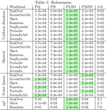
Figure 1 depicts snapshots of the creation phase, the re-finement phase, and the consolidation phase of Progressive Quicksort. We discuss all three phases in detail in the fol-lowing paragraphs.
Creation Phase
In the first iteration, we allocate an uninitialized column of the same size as the original column and select a pivot. The pivot is selected by taking the average value of the smallest and largest value of the column. In Figure 1, pivot 10 is the average of 1 and 19. If sufficient statistics are available, the median value of the column could be used instead. Unlike adaptive indexing, the pivot selection is not impacted by the query predicates. We then scan the original column and copy the firstN∗δ elements to either the top or bottom of the index depending on their relation to the pivot. In this step, we also search for any elements that fulfill the query predicate and afterwards scan the not-yet-indexed 1−ρfraction of the column to compute the complete answer to the query. In subsequent iterations, we scan either the top, bottom, or both parts of the index based on how the query predicate relates to the chosen pivot.
Cost Model. The total time taken in the creation phase
is the sum of (1) the scan time of the base table, (2) the index lookup time and (3) the additional indexing time. The scan time is given by multiplying the amount of pages we need to scan (Nγ) by the amount of time it takes for a sequential page access (ω), resulting in tscan=ω∗Nγ. The pivoting time, i.e., index construction time, consists of scanning the pages of the base table and writing the pivoted elements to the result array. The pivoting time is therefore obtained by multiplying the time it takes to scan and write a page sequentially (κ+ω) by the amount of pages we need to write, resulting intpivot= (κ+ω)∗Nγ.
The total time taken for the initial indexing process is given by multiplying the scan time by the fraction of the base table we need to scan. Initially, we need to scan the entire base table, but as the fraction of indexed data (ρ) increases, we need to scan less. Instead, we scan the index to answer the query. The amount of data we need to scan in the index depends on how the query predicates relate to the pivot. The fraction of data that we need to scan is given byα, and can be computed for a given set of query predicates. The total
16 19 7 1 4 13 13 1 14 8 9 11 1 6 3 6 3 16 13 2 1 8 19 7 12 11 4 9 14 Original Column A ≤ 10 10 < A 6 16 2 Uninitialized Initialize 3 2 8 9 14 11 12 13 Initialize 2 A ≤ 10 10 < A A ≤ 7 7 < A A ≤ 15 15 < A Refinement Pivot=10 Pivot=15 Pivot=7 14 13 4 6 1 2 3 7 8 12 16 19 Consolidation Sor ted 1 6 11 14 B+ T ree A ≤ 10 10 < A Pivot=10 7 6 3 2 4 9 11 12 19 16
Figure 1: Progressive Quicksort.
fraction of the data that we scan is 1−ρ+α−δ. The fraction of the data that we index in each step isδ. Hence the total time taken is given byttotal= (1−ρ+α−δ)∗tscan+δ∗tpivot.
Indexing Budget. In this phase, we set delta such that
δ=tbudget
tpivot. For the fixed indexing budget, we select thisδ
for the first query and keep on using thisδfor the remainder of the workload. For the adaptive indexing budget, we use this formula to select theδ for each query.
Refinement Phase
We refine the index by recursively continuing the quicksort in-place in the separate sections. The refinement consists of swapping elements in-place inside the index around the pivots of the different segments. When the pivoting of a segment is completed, we recursively continue the quicksort in the child segments. We maintain a binary tree of the pivot points. In the nodes of this tree, we keep track of the pivot points and how far along the pivoting process we are. To do an index lookup, we use this binary tree to find the sections of the array that could potentially match the query predicate and only scan those, effectively reducing the amount of data to be accessed even when the full pivoting has not been completed yet.
When we reach a node that is smaller than the L1 cache, we sort the entire node instead of recursing any further. After sorting a node entirely, we mark it as sorted. When two children of a node are sorted, the entire node itself is sorted, and we can prune the child nodes. As the algorithm progresses, leaf nodes will keep on being sorted and pruned until only a single fully sorted array remains.
Cost Model. In the refinement phase, we no longer need
to scan the base table. Instead, we only need to scan the fractionαof the data in the index. However, we now need to (1) traverse the binary tree to figure out the bounds ofα, and (2) swap elements in-place inside the index instead of sequentially writing them to refine the index. The cost for traversing the binary tree is given by the height of the binary treehtimes the cost of a random page accessφ, resulting in
tlookup=h∗φ. For the swapping of elements, we perform predicated swapping to allow for a constant cost regardless of how many elements we need to swap. Therefore the cost for swapping is equivalent to the cost of sequential writing, i.e.,tswap=κ∗Nγ. The total cost in this phase is therefore equivalent tottotal=tlookup+α∗tscan+δ∗tswap.
Indexing Budget. In this phase, we set delta such that
δ=tbudget
tswap for the adaptive indexing budget.
Consolidation Phase
In the consolidation phase we construct a B+-tree index on top of our sorted array. In order to progressively construct the B+-Tree we copy every βelement of our sorted array to a parent level. In total we copy Ncopy =P
logβ(n)
i=1 (
n βi)
elements. This process is depicted in the consolidation phase of Figure 1 whereβ= 4 and the parent node of the array indexes every 4th element (i.e., offsets 0, 4, 8 and 12).
Cost Model. In the consolidation phase, we use
bi-nary search in the sorted array until the B+-Tree levels are complete. This results in tlookup = log2(n)∗φ. To
construct the B+-Tree we copy every βelement from one level to the next, therefore the cost of copying the ele-ments is the cost of access a random element from the cur-rent level and sequentially write it to the next, defined by
tcopy=Ncopy∗κ∗γThe total cost in this phase is equivalent tottotal=tlookup+α∗tscan+δ∗tcopy.
Indexing Budget. In this phase, we set delta such that
δ= tbudget
tcopy for the adaptive indexing budget.
3.2
Progressive Radixsort (MSD)
Figure 2 depicts snapshots of the creation phase, the re-finement phase, and the consolidation phase of Progressive Radixsort (MSD). We discuss all three phases in detail in the following paragraphs.
Creation Phase
In the creation phase of progressive radixsort, we perform the radixsort partitioning into buckets that are located in separate memory regions. We start by allocatingbempty buckets. Then, while scanning the original column, we place
N∗δelements into the buckets based on their most significant log2b bits. We then scan the remaining 1−ρ fraction of
the base column. In subsequent iterations, we scan the [0, b] buckets that could potentially contain elements matching the query predicate to answer the query in addition to scanning the remainder of the base column.
Bucket Count. Radix clustering performs a random
memory access pattern that randomly writes inb output buckets. To avoid excessive cache- and TLB-misses, assuming that each bucket is at least of the size of a memory page, the numberbof buckets, and thus the number of randomly accessed memory pages, should not exceed the number of cache lines and TLB entries, whichever is smaller [2]. Since our machine has 512 L1 cache lines and 64 TLB entries, we useb= 64 buckets.
Bucket Layout.To avoid having to allocate large regions
of sequential data for every bucket, the buckets are imple-mented as a linked list of blocks of memory that each hold up tosbelements. When a block is filled, another block is added to the list and elements will be written to that block. This adds some overhead over sequential reads/writes as every
sbelements there will be a memory allocation and random access, and for every element that is added the bounds of the current block have to be checked.
Cost Model. In the creation phase, the total time taken
is the sum of (1) the scan time of the base table, (2) the index lookup time and (3) the time it takes to add elements to buckets. The scan time of the base table is equivalent to the
11 4 1 13 8 14 11 3 16 16 13 3 19 8 14 14 1 6 3 14 13 2 1 8 19 7 12 11 4 16 9 6 2 Initialize Refinement 00… 13 11 1 7 6 3 2 4 12 9 01… 10… 11… Uninitialized 19 00. 01. 10. 11. 1 2 4 6 7 00. 01. 10. 11. 9 12 00… 01… 10… Refinement 13 8 14 11 3 00. 01. 10. 11. 1 2 4 6 7 00. 01. 10. 11. 9 12 9 16 13 6 2 3 7 8 12 14 19 Original Column
Figure 2: Progressive Radixsort (MSD).
scan time (tscan) given in Section 3.1. Scanning the buckets for the already indexed data has equivalent performance to performing a sequential scan plus the random accesses we need to perform everysbelements, hence the scan time of the buckets is equivalent totbscan=tscan+φ∗sN
b. As we
determine which bucket an element belongs to only based on the most significant bits, finding the relevant bucket for an element can be done using a single bitshift. As we chose the bucket count such that all bucket regions can fit in cache, the cost of writing elements to buckets is equivalent to the cost of sequentially writing them (κ). We need to perform a memory allocation everysb entries, which has a cost ofτ. This results in a total cost of bucketing equal to
tbucket = (κ+ω)∗Nγ +τ∗sN
b. The total cost is therefore
ttotal= (1−ρ−δ)∗tscan+α∗tbscan+δ∗tbucket.
Indexing Budget. In this phase, we set delta such that
δ=tbudget
tbucket. For the fixed indexing budget, we select thisδ
for the first query and keep on using thisδfor the remainder of the workload. For the adaptive indexing budget, we use this formula to select theδ for each query.
Refinement Phase
In the refinement phase, all elements in the original column have been appended to the buckets. In this phase, we re-cursively partition by the next set of log2bmost significant digits. For each of the buckets, this results in the creation of another set ofbbuckets in each of the refinement phases, for a total ofb∗bbuckets in the second phase. To avoid the overhead of managing these buckets to become bigger than the overhead of actually performing the radix partitioning, we avoid re-partitioning buckets that fit into the L1 cache and instead immediately insert the values of these buckets in sorted order into the final sorted array, as shown in Figure 2. As the buckets themselves are ordered (i.e., for two bucketsbi andbi+1, we knowei< ei+1∀ei∈bi, ei+1∈bi+1), we know
the position of each bucket in the final sorted array without having to consider any elements in the other buckets.
We keep track of the buckets using a tree in which the nodes point towards either the leaf buckets or towards a position in the final sorted array in case the leaf buckets have already been merged in there. This tree is used to answer queries on the intermediate structure. When we get a query, we look up which buckets we have to scan based on the most significant bits of the query predicates. We then scan the buckets or the final index, where required.
When the first iteration of the refinement phase is com-pleted, we recursively continue with the next set of log2b
most significant digits until all the elements have been merged and sorted into the final index. At that point, we construct our B+-tree index from the single fully sorted array.
Cost Model. The total time taken for a query is the
sum of (1) the time taken to scan the required buckets to answer the query predicates and (2) the time taken to perform the radix partitioning of the elements. The time taken to scan the buckets is the same as in the creation phase,α∗tbscan. The time taken for the radix partitioning istbucket= (κ+ω)∗Nγ +τ∗sN
b. The total cost is therefore
ttotal=α∗tbscan+δ∗tbucket.
Indexing Budget. In this phase, we set delta such that
δ=tbudget
3.3
Progressive Bucketsort
Progressive Bucketsort (Equi-Height) is very similar to Progressive Radixsort (MSD). The main difference is in the way the initial partitions (buckets) are determined. Instead of radix clustering, which is fast but yields equally sized partitions only with uniform data distributions, we perform a value-based range partitioning to yield equally sized parti-tions also with skewed data, at the expense that determining the bucket that a value belongs to is more expensive. Figure 3 depicts a snapshot of the creation phase and two snapshots of the refinement phase. In the following, we discuss these two phases in detail. The consolidation phase is the same as with Progressive Quicksort and Progressive Radixsort (MSD).
Bucket Count. To optimize for writing and reading from
the buckets, our implementation of progressive bucketsort uses 64 buckets, as discussed in Section 3.2.
Creation Phase
Progressive Bucketsort operates in a very similar way to Progressive Radixsort (MSD). Instead of choosing the bucket an element belongs to based only on the most significant bits, the bucket is chosen based on a set of bounds that more-or-less evenly divide the elements of the set into the separate buckets. These bounds can be obtained either in the scan to answer the first query or from existing statistics in the database (e.g., a histogram).
Cost Model. In the creation phase, the cost of the
algorithm is identical to that of Progressive Radixsort (MSD) except that determining which element a bucket belongs to now requires us to perform a binary search on the bucket boundaries, costing an additional log2btime per element
we bucket. This results in the following cost for the initial indexing processttotal= (1−ρ−δ)∗tscan+α∗tbscan+δ∗ log2b∗tbucket.
Indexing Budget. In this phase, we set delta such that
δ= tbudget
log2b∗tbucket. For the fixed indexing budget, we select
thisδ for the first query and keep on using thisδ for the remainder of the workload. For the adaptive indexing budget, we use this formula to select theδfor each query.
13 14 16 8 7 16 3 4 6 11 4 19 13 7 6 9 4 6 1 2 6 3 14 13 2 1 8 19 7 12 11 4 16 9 Original Column 3 1 Initialize Refinement 2 3 12 19 Refinement A<5 9 11 3 2 1 8 12 14 A<5 A < 3 3<=A 5<=A<10 10<=A<14 14<=A<20 2 1 A < 5 5<=A Uninitialized Sor ted A < 10 10<=A 13 14 5<=A<10 10<=A<14 14<=A<20 Sor ted A < 8 8<=A A < 5 5<=A
Figure 3: Progressive Bucket Sort
Refinement Phase
In the refinement phase, all elements in the original column have been appended to the buckets. We then merge the buckets into a single sorted array. Unlike with Progressive Radixsort (MSD), we do not recursively keep on using pro-gressive bucketsort. This is because the overhead of finding and maintaining the equi-height bounds for each of the sub-buckets is too large. Instead, we sort the individual sub-buckets into the final sorted list using Progressive Quicksort. Using a progressive algorithm to sort individual buckets protects us from performance spikes caused by sorting large buckets. The buckets are merged into the final sorted index in order, as such, we always have at most a single iteration of Progressive Quicksort active at a time in which we are performing swaps. As we are using Progressive Quicksort, the cost model for this phase is equivalent to the cost model of Progressive Quicksort. After all the buckets have been merged and sorted into the final index, we have a single fully sorted array from which we can construct our B+-tree index.
3.4
Progressive Radixsort (LSD)
Progressive Radixsort Least Significant Digits (LSD) per-forms a progressive radix clustering on the least significant bits during the creation phase. Given that this does not result in a range partitioning, as with radix cluster (MSD), we cannot perform Progressive Quicksort in the individual buckets to refine them in-place. Instead, we perform out-of-place radix (LSD) clustering also during the refinement phase, to achieve a ”pure” Radixsort (LSD) in a progressive manner. Figure 4 depicts a snapshot of the creation phase and two snapshots of the refinement phase. In the following, we discuss these two phases in detail. The consolidation phase is the same as above.
Bucket Count. To optimize for writing and reading
from the buckets our implementation of progressive radixsort (LSD) uses 64 buckets, as discussed in Section 3.2.
Creation Phase
The creation phase of this algorithm is similar to the creation phase of Progressive Radixsort (MSD) except that we parti-tion elements based on the least-significant bits instead of the most-significant bits. We can use the buckets that are cre-ated to speed up point queries because we only need to scan
9 19 3 13 7 13 6 14 1 6 2 6 3 14 13 2 1 8 19 7 12 11 4 16 9 Original
Column Initialize Refinement Refinement
…00 8 13 2 3 …00 …01 …10 …11 14 …01 …10 …11 3 1 19 12 11 4 16 9 .00.. .01.. .10.. .11.. 8 12 4 16 6 0…. 1…. 4 8 16 6 12 13 .00.. .01.. .10.. .11.. 1 14 2 7 11 16 19 1 2 3 4 6
the bucket in which the query value falls. However, unlike the buckets created for the Progressive Radixsort (MSD) and Progressive Bucketsort, these intermediate buckets cannot be used to speed up range queries in many situations. Because the elements are inserted based on their least-significant bits, the buckets do not form a value-based range-partitioning of the data. Consequently, we will have to scan many buckets, depending on the domain covered by the range query.
The cost model for the Progressive Radixsort (LSD) is also equivalent to the cost model of the Progressive Radixsort (MSD), except the value ofαis likely to be higher for range queries (depending on the query predicates) as the elements that answer the query predicate are spread in more buckets. As scanning the buckets is slower than scanning the original column, we also have a fallback that whenα==ρwe scan the original column instead of using the buckets to answer the query.
Refinement Phase
In the refinement phase, we move elements from the cur-rent set of buckets to a new set of buckets based on the next set of significant bits. We repeat this process until the column is sorted. How many iterations this takes de-pends on the bucket count and the value domain of the column, which we obtain from the [min, max] values. We can compute the amount of required iterations with the formula dlog2(max−min)/log2(b)e. For example, for a
column with values in the range of [0,216) and 64 buck-ets, the amount of iterations required before convergence is
dlog2(216)/log2(64)e= 3.
Cost Model. In this phase, we scanα fraction of the
original buckets to answer the query and moveδ fraction of the elements into the new set of buckets. This results in the following cost for the refinement process: ttotal =
α∗tbscan+δ∗tbucket.
Indexing Budget. In this phase, we set delta as δ =
tbudget
tbucket for the adaptive indexing budget.
4.
EXPERIMENTAL EVALUATION
In this section, we provide an evaluation of the proposed Progressive Indexing methods and the performance charac-teristics they exhibit. In addition, we provide a comparison of the performance of the proposed methods with adaptive indexing methods.
Setup. We implemented all our Progressive Indexing
algorithms in a stand-alone program written in C++. We in-cluded implementations of the adaptive indexing algorithms, provided by the authors, and implemented an adaptive crack-ing kernel algorithm that picks the most efficient kernel when executing a query, following the decision tree from Haffner et al. [11]. Both the progressive indexing algorithms and the existing techniques were compiled with GNUg++version 7.2.1 using optimization level-O3. All experiments were con-ducted on a machine equipped with 256 GB main memory and an 8-core Intel Xeon E5-2650 v2 CPU @ 2.6 GHz with 20480 KB L3 cache.
4.1
Workloads
In the performance evaluation, we use two data sets.
SkyServer. The Sloan Digital Sky Survey2 is a project
that maps the universe. The data set and interactive data
ex-2
https://www.sdss.org/
(a) Data Distribution
0 108 0 50000 100000 150000 Query (#) Quer y Range (b) Workload Figure 5: Skyserver
ploration query logs are publicly available via the SkyServer3 website. Similar to Halim et al. [12] we focus the benchmark on the range queries that are applied on theRight Ascension
column of the PhotoObjAll table. The data set contains almost 600 million tuples, with around 160,000 range queries that focus on specific sections of the domain before moving to different areas. The data and the workload distributions are shown in Figure 5.
Synthetic. The synthetic data set is composed of two
data distributions, consisting of 108 or 109 8-byte integers
distributed in the range of [0, n), i.e., for 109the values are in the range of [0,109). We use two different data sets. The first one is composed of unique integers that are uniformly distributed, while the second one follows a skewed distri-bution with non-unique integers where 90% of the data is concentrated in the middle of the [0, n) range. The synthetic workload consists of 106queries in the formSELECT SUM(R.A)
FROM R WHERE R.A BETWEEN V1 AND V2. The values forV1
andV2 are chosen based on the workload pattern. The
dif-ferent workload patterns and their mathematical description are depicted in Figure 6.
4.2
Impact of Delta (
δ)
Theδ parameter determines the performance character-istics shown by the Progressive Indexing algorithms. For
δ= 0, no indexing is performed, meaning that algorithms resort to performing full scans on the data, never converging to a full index. For δ = 1, the entire creation phase will be completed immediately during the first query execution. Between these two extremes, we are interested in seeing how different values of theδparameter influence the performance characteristics of the different algorithms.
In order to measure the impact of differentδparameters on the different algorithms, we execute the SkyServer workload using a δ∈ [0.005,1]. We measure the time taken for the first query, the amount of queries until pay-off, the amount of queries necessary for full convergence, and the total time spent executing the entire workload.
First Query. Figure 7a shows the performance of the
first query for varying values ofδ. The performance of the first query degrades as δ increases since each query does extra work proportional toδ. For every algorithm, however, the amount of extra work done differs.
We can see that Bucketsort is impacted the most by in-creasing δ. This is because determining which bucket an element falls into costsO(log b) time, followed by a random write for inserting the element into the bucket. Radixsort, despite its similar nature to Bucketsort, is impacted much less heavily by an increasedδ. This is because determining which bucket an element falls into costs constantO(1) time.
3
Figure 6: Synthetic Workloads [12]. ● ● ● ● ● ● ● ● ● ● ● ● ● 3 6 9 12 0.01 0.10 1.00 δ Quer y Time (s) ●P. Bucket P. Quick P. Radix (LSD) P. Radix (MSD)
(a) First query.
● ● ● ● ●● ●●●●●●● 0 250 500 750 0.01 0.10 1.00 δ Quer y Number (#) ●P. Bucket P. Quick P. Radix (LSD) P. Radix (MSD) (b) Pay-off. ● ● ● ● ● ● ●●●●●●● 0 1000 2000 3000 4000 5000 0.01 0.10 1.00 δ Quer y Number (#) ●P. Bucket P. Quick P. Radix (LSD) P. Radix (MSD) (c) Convergence. ● ● ● ● ● ● ●●●●●●● 0 250 500 750 0.01 0.10 1.00 δ T otal Time (s) ●P. Bucket P. Quick P. Radix (LSD) P. Radix (MSD) (d) Cumulative time.
Figure 7: Progressive indexing experiments with varying deltas (X-axes in logarithmic scale).
Quicksort experiences the lowest impact from an increasingδ, as elements are always written to only two memory locations (the top and bottom of the array), the extra sequential writes
are not very expensive.
Pay-Off. Figure 7b shows the number of queries required
until the Progressive Indexing technique becomes worth the investment (i.e., the query numberqfor whichP
qtprog ≤
P
qtscan) for varying values of δ. We observe that with a very small δ, it takes many queries until the indexing pays off. While a smallδ ensures low first query costs, it significantly limits the progress of index-creation per query, and consequently the speed-up of query processing. With increasing δ, the number of queries required until pay-off quickly drops to a stable level.
We see that Radixsort (LSD) needs a very high amount of queries to pay-off for low values of δ. This is because the intermediate index that is created cannot be used to accelerate wide range queries until the index is converged. When the value of δ is high, the index converges faster and hence can be utilized to answer range queries earlier. Quicksort also has a high time to pay-off with a low delta because the intermediate index can only be used to accelerate range queries that do not contain the pivots, hence in early stages of the index the full table often needs to be scanned. Bucketsort and Radixsort (MSD) do not suffer from these problems, hence they pay-off fast even with lower values for
δ.
Convergence. Theδparameter affects the convergence
speed towards a full index. Whenδ= 0 the index will never
converge, and a higher value for δwill cause the index to converge faster as more work is done per query on building the index.
Figure 7c shows the number of queries required until the index converges towards a full index. We see that Radixsort converges the fastest, even with a low δ. It is followed by Quicksort and then Bucketsort.
The reason Radixsort converges in so few iterations is because it uses radix partitioning, which means that after
dlog2(n)/log2(b)e = dlog2(109)/log2(64)e = 5 partitioning
rounds the index is fully converged. The other algorithms use quicksort pivoting, which requires more passes over the data.
Cumulative Time. As we have seen before, a high value
for δ means that more time is spent on constructing the index, meaning that the index converges towards a full index faster. While earlier queries take longer with a higher value ofδ, subsequent queries take less time. Another interesting measurement is the cumulative time spent on answering a large number of queries. Does the increased investment in index creation earlier on pay off in the long run?
Figure 7d depicts the cumulative query cost. We can see that a higher value of δ leads to a lower cumulative time. Converging towards a full index requires the same amount of time spent on constructing the index, regardless of the value ofδ. However, whenδis higher, that work is spent earlier on (during fewer queries), and queries can benefit from the constructed index earlier.
Progressive Quicksort and Radixsort (LSD) perform poorly when the delta is low. For Quicksort, this is because it will
take many queries to finish our pivoting in one element. While in Radixsort (LSD) the intermediate index that is created cannot be effectively used to answer range queries be-fore it fully converges, meaning a long time until convergence results in poor cumulative time. Progressive Bucketsort and Radixsort (MSD) perform better than Progressive Quicksort for all values ofδ, with Radixsort (MSD) slightly outper-forming Bucketsort.
Another observation here is that the cumulative time con-verges rather quickly with an increasing delta. The cumu-lative time withδ = 0.25 andδ = 1 are almost identical for all algorithms, while the penalization of the initial query continues to increase significantly (recall Figure 7a).
4.3
Cost Model Validation
For both the fixed indexing budget and the adaptive index-ing budget, we need the cost models presented in Section 2.2 to estimate the actual query processing and index creation costs. For the fixed indexing budget, we need the cost model to compute the initial value ofδ based on the desired in-dexing budget. For the adaptive inin-dexing budget, we need the cost model to adapt the value ofδfor each query to the current minimum query cost.
In this set of experiments, we experimentally validate our cost models. In order to use the cost models in practice, we need to first obtain values for all of the constants that are used, such as the scanning speed and the cost of a cache miss. Since these constants depend on the hardware, we perform these operations when the program starts up and measure how long it takes to perform these operations. The measured values are then used as the constants in our cost model.
Fixed Indexing Budget. Before diving into the details
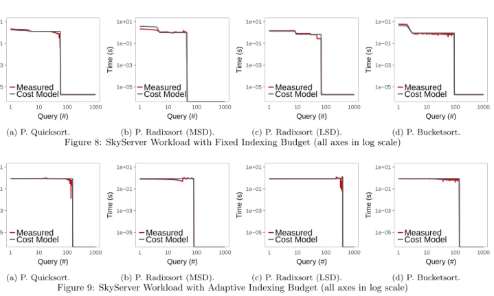
of choosing a variableδper query for the adaptive indexing budget, we first experimentally validate our cost models. We run the SkyServer benchmark with a constantδ= 0.25 for the entire query sequence and compare the measured execution times with the times predicted by our cost models. Figure 8 shows the results for all four Progressive Index-ing techniques we propose. The graphs clearly depict the individual phases of our algorithms (cf., Section 3) and show that significant improvements in query performance happen mostly with the transition from one phase to the next. Given thatδdetermines the fraction of data that is to be consid-ered for index refinement with each query (rather than a fraction of the full scan cost), the different techniques depict different per query cost, depending on the respective index refinement operations performed as well as the efficiency of the respective partially built indexes. The graphs also show that our cost models predict the actual costs well, accurately predicting each phase transition as well as the point when the full index has been finalized, and no further indexing is required.
Adaptive Indexing Budget. With our cost models
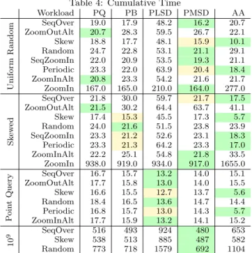
val-idated, we now run the SkyServer benchmark with all four Progressive Indexing techniques with the adaptive indexing budget. We selecttbudget= 0.2∗tscan, i.e., the indexing bud-get is selected as 20% of the full scan cost. Figure 9 depicts the results of this experiment for each of the algorithms. In all graphs, we observe that the total execution time stays close to constant at a high level, matching the given budget until the index is fully built, and no further refinement is required.
In Figure 9a, the measured and predicted time are shown
for the Progressive Quicksort algorithm. Initially, the cost model accurately predicts the performance of the algorithm. However, close to convergence, the cost model predicts a slightly higher execution time. This is because as the pieces become smaller, they start fitting inside the CPU caches entirely, which results in faster swaps than predicted by our cost model.
In Figure 9b, the measured and predicted time are shown for the Progressive Radixsort (MSD) algorithm. In the initialization phase, the cost model matches the measured time initially, but the measured time slightly decreases below the cost model as the initialization progresses. This is because the data distribution is relatively skewed, which results in the same buckets being scanned for every query, which will then be cache resident and faster than predicted. In the refinement phase, there are some minor deviations from the cost model caused by smaller radix partitions fitting in CPU caches, which our cost model does not accurately predict.
In Figure 9c, the measured and predicted time are shown for the Progressive Radixsort (LSD) algorithm. The cost model accurately predicts the performance of the initializa-tion and refinement phases of the algorithm but results in several spikes later in the refinement phase. These spikes occur because the workload we are using consists of very wide range queries. These range queries can only take advantage of the LSD index depending on the exact range queries issued. Because of this, certain queries can be answered much faster using the index, whereas others cannot use the index at all. As our cost model is pessimistic, this results in the measured time being faster than the predicted time.
In Figure 9d, the measured and predicted time are shown for the Progressive Bucketsort algorithm. In the initialization phase, the cost model closely matches the measured time. After it, Progressive Quicksort is used to merge the different buckets into a single sorted array. The different iterations of Progressive Quicksort each have small downwards spikes when the pieces start fitting inside the CPU caches.
4.4
Adaptive Indexing Comparison
In the remainder of the experiments section, we will be comparing the progressive indexing techniques with existing adaptive indexing techniques. In particular, we focus on standard cracking (STD), stochastic cracking (STC), pro-gressive stochastic cracking (PSTC), coarse granular index (CGI) and adaptive adaptive indexing (AA).
The implementations for the Full Index, Standard Crack-ing, Stochastic CrackCrack-ing, and Coarse Granular Index were inspired by the work done in Schuhknecht et al. [24]4. The
implementation for Progressive Stochastic Cracking was in-spired by the work done in Halim et al. [12]5. Progressive stochastic cracking is run with the allowed swaps set to 10% of the base column. The implementation for the adaptive adaptive indexing algorithm has been provided to us by the authors of the Adaptive Adaptive Indexing work [23], and we use the manual configuration suggested in their paper.
We compare all the progressive indexing techniques that we have introduced in this work: Progressive Quicksort (PQ), Progressive Bucketsort (PB), Progressive Radixsort LSD (PLSD) and Progressive Radixsort MSD (PMSD). For each of the techniques, we use an adaptive indexing budget where
4
https://infosys.uni-saarland.de/publications/ uncracked_pieces_sourcecode.zip
5
1e−05 1e−03 1e−01 1e+01 1 10 100 1000 Query (#) Time (s) Measured Cost Model (a) P. Quicksort. 1e−05 1e−03 1e−01 1e+01 1 10 100 1000 Query (#) Time (s) Measured Cost Model (b) P. Radixsort (MSD). 1e−05 1e−03 1e−01 1e+01 1 10 100 1000 Query (#) Time (s) Measured Cost Model (c) P. Radixsort (LSD). 1e−05 1e−03 1e−01 1e+01 1 10 100 1000 Query (#) Time (s) Measured Cost Model (d) P. Bucketsort.
Figure 8: SkyServer Workload with Fixed Indexing Budget (all axes in log scale)
1e−05 1e−03 1e−01 1e+01 1 10 100 1000 Query (#) Time (s) Measured Cost Model (a) P. Quicksort. 1e−05 1e−03 1e−01 1e+01 1 10 100 1000 Query (#) Time (s) Measured Cost Model (b) P. Radixsort (MSD). 1e−05 1e−03 1e−01 1e+01 1 10 100 1000 Query (#) Time (s) Measured Cost Model (c) P. Radixsort (LSD). 1e−05 1e−03 1e−01 1e+01 1 10 100 1000 Query (#) Time (s) Measured Cost Model (d) P. Bucketsort.
Figure 9: SkyServer Workload with Adaptive Indexing Budget (all axes in log scale)
we settbudget= 0.2∗tscan, i.e., the cost of each query will be equivalent to 1.2∗tscanuntil convergence.
For reference, we also include the timing results when only performing full scans on the data (FS) and when constructing a full index immediately on the first query (FI). The full scan implementation uses predication to avoid branches, and the full index bulk loads the data into a B+-tree after which the B+-tree is used to answer subsequent queries.
Metrics. The metrics that we are interested in are the
time taken for the first query, the amount of queries required until convergence, the robustness of each of the algorithms and the cumulative response time. The robustness we com-pute by taking the variance of the first 100 query times.
SkyServer Workload
Table 2: SkyServer Results
Index First Q Convergence Robustness Cumulative
FS 0.75 x 0 118743.7 FI 34.10 1 x 121.4 STD 5.26 x 0.290 1082.2 STC 4.99 x 0.250 245.6 PSTC 4.89 x 0.240 254.5 CGI 5.71 x 0.320 1008.9 AA 8.50 x 0.800 188.4 PQ 0.90 150 0.002 202.9 PMSD 0.90 119 0.030 157.5 PLSD 0.81 368 3.4e-05 377.4 PB 0.83 138 0.009 166.4
In the first part of the experiments section, we execute the full SkyServer workload using each of the different indexing techniques. The results for each of the indexing techniques are shown in Table 2. The algorithms have been divided into three sections: the baseline, the adaptive indexing techniques, and the progressive indexing techniques.
The results for the baseline techniques are not very sur-prising. The full scan method is the most robust method, as we use predication, and no index is constructed the cost of each query is identical. The full scan method is also the cheapest method when it comes to the cost of the first query as no time is spent on indexing at all. The full scan, how-ever, takes significantly longer to answer the full workload than the other methods. Answering the full workload takes almost 30 hours, whereas all the other techniques finish the entire workload in under 20 minutes. The full index lies at the other extreme. It takes 50xlonger to answer the first query while the index is being constructed, however, it has the lowest cumulative time as the index can be utilized to quickly answer all of the remaining queries.
For the adaptive indexing techniques, we can see that their first query cost is significantly lower than that of a full index, but still significantly higher than that of a full scan. Each of the adaptive indexing methods perform a significant amount of work copying the data and cracking the index on the first query that result in a very high cost for the first query. They do achieve a significantly faster cumulative time than the full scans, however, in sum, they take longer than the full index to answer the workload. Standard cracking and coarse granular indexing perform particularly poorly because of the sequential nature of the workload, as shown in Figure 5. Stochastic cracking and adaptive indexing perform better as they do not choose the pivots based on the query predicates. Adaptive adaptive indexing has the best cumulative perfor-mance, which is consistent with the results in Schuhknecht et al. [23].
The progressive indexing methods all have approximately the same cost for the first query, which is 1.2x the scan cost. This is by design as we set the indexing budget
tbudget = 0.2∗tscan for each of the algorithms. The main difference between the algorithms is the robustness and the
● Index (0.000003) 1.2x Scan (0.9) 10 1000 Query (#) Quer y Time (log(s)) ●AA Idx P. Quick P. Stc 10%
Figure 10: Progressive Quicksort vs Adaptive Indexing. (all axes in log scale)
time until convergence. As we are executing range queries, the Radixsort LSD performs the worst. The LSD partition-ing cannot assist in answerpartition-ing the range queries, and hence, the intermediate index does not speed up the workload prior to convergence. Radixsort MSD performs the best, as the data set is rather uniformly distributed the radix partitioning works to very efficiently create a partitioning of the data, which can be immediately utilized to speed up subsequent queries. For each of the progressive indexing methods, we see that they converge relatively early in the workload. As we have set every query to take 1.2∗tscanuntil convergence, a significant amount of time can be spent on constructing the index for each query, especially in later queries when the intermediate index can already be used to efficiently ob-tain the answer. We also note that the progressive indexing methods each have a significantly higher robustness score than the adaptive indexing methods. Progressive indexing presents up to 4 orders of magnitude lower query variance when compared to the adaptive indexing techniques. This is achieved by our cost model balancing the per query execu-tion cost to be (almost) the same until convergence, while adaptive indexing suffers from many performance spikes.
The execution time for each of the queries in the SkyServer workload is shown in Figure 10. For clarity, we focus on the best adaptive indexing methods (Adaptive Adaptive Index-ing in terms of cumulative time, and Progressive Stochastic 10% in terms of first query cost and robustness) and progres-sive quicksort. We can see that both the adaptive indexing methods start with a significantly higher first query cost, and then fall quickly. Neither of them sufficiently converges, however, and both continue to have many performance spikes. Progressive quicksort, on the other hand, starts at the speci-fied budget and maintains that query cost until convergence, after which the cost drops to the cost of a full index.
Synthetic Workloads
In the second part of our experiments, we execute all syn-thetic workloads described in Section 4.1. All results are presented in tables, each table is divided into four parts, each representing one set of experiments. The first three are on data with 108elements and use random distribution, skewed
distribution, and only point queries respectively. The final one is on 109 elements on random distribution. With the exception of point queries and the ZoomIn and SeqZoomIn workloads, all queries have 0.1 selectivity. From the adaptive indexing techniques, adaptive adaptive indexing presents the
best cumulative time. Hence we select it for comparison. As previously, we set the indexing budgettbudget= 0.2∗tscan for each progressive indexing algorithm.
Table 3: First query cost
Workload PQ PB PLSD PMSD AA Uniform Random SeqOver 0.15 0.15 0.14 0.14 1.4 ZoomOutAlt 0.15 0.15 0.14 0.14 1.4 Skew 0.15 0.15 0.14 0.14 1.4 Random 0.15 0.15 0.14 0.14 1.4 SeqZoomIn 0.15 0.15 0.14 0.14 1.4 Periodic 0.15 0.15 0.14 0.14 1.4 ZoomInAlt 0.15 0.15 0.14 0.14 1.4 ZoomIn 0.15 0.15 0.14 0.14 1.4 Sk e w ed SeqOver 0.15 0.15 0.14 0.14 1.5 ZoomOutAlt 0.15 0.15 0.14 0.13 1.5 Skew 0.15 0.15 0.14 0.13 1.5 Random 0.15 0.15 0.13 0.13 1.5 SeqZoomIn 0.15 0.15 0.14 0.13 1.5 Periodic 0.15 0.15 0.14 0.13 1.5 ZoomInAlt 0.15 0.15 0.14 0.14 1.5 ZoomIn 0.15 0.15 0.14 0.14 1.5 P oin t Query SeqOver 0.15 0.15 0.21 0.14 1.4 ZoomOutAlt 0.15 0.15 0.21 0.14 1.4 Skew 0.15 0.15 0.21 0.14 1.4 Random 0.15 0.15 0.21 0.14 1.4 Periodic 0.15 0.15 0.21 0.14 1.4 ZoomInAlt 0.15 0.15 0.21 0.14 1.4 10 9 SeqOver 1.5 1.5 1.4 1.7 13.9 Skew 1.5 1.5 1.4 1.7 13.8 Random 1.5 1.5 1.4 1.7 25.4
Table 3 depicts the cost of the first query for all algorithms. All progressive indexing algorithms present a similar first query cost. Which accounts for approximately 1.2xthe scan cost, as chosen in our setup. Adaptive indexing has a higher cost due to the complete copy of the data and by completing a full partition step in the first query. In general, progressive indexing has one order of magnitude faster first query cost than adaptive indexing.
Table 4: Cumulative Time
Workload PQ PB PLSD PMSD AA Uniform Random SeqOver 19.0 17.9 48.2 16.2 20.7 ZoomOutAlt 20.7 28.3 59.5 26.7 22.1 Skew 18.8 17.7 48.1 15.9 10.1 Random 24.7 22.8 53.1 21.1 29.1 SeqZoomIn 22.0 20.9 53.5 19.3 21.1 Periodic 23.3 22.0 63.9 20.4 18.4 ZoomInAlt 20.8 23.3 54.2 21.6 21.7 ZoomIn 167.0 165.0 210.0 164.0 277.0 Sk ew ed SeqOver 21.8 30.0 59.7 21.7 17.5 ZoomOutAlt 21.5 30.2 64.4 63.7 41.1 Skew 17.4 15.3 45.5 17.3 5.7 Random 24.0 21.6 51.5 23.8 23.9 SeqZoomIn 23.3 21.2 52.6 23.1 18.3 Periodic 23.3 21.3 64.2 23.3 17.0 ZoomInAlt 22.2 25.1 54.8 21.8 33.5 ZoomIn 938.0 919.0 934.0 917.0 1655.0 P o in t Query SeqOver 16.7 15.7 13.2 14.0 15.1 ZoomOutAlt 17.7 15.8 13.0 14.0 15.5 Skew 16.6 15.5 12.7 13.7 5.6 Random 18.4 16.5 13.6 14.7 14.4 Periodic 16.8 15.7 13.0 14.3 5.7 ZoomInAlt 17.7 15.9 13.2 14.1 15.2 10 9 SeqOver 516 493 924 480 653 Skew 538 513 885 487 582 Random 773 718 1579 692 1104
Table 4 depicts the cumulative time of fully executing each workload. Under uniform random data, we can see that
progressive indexing outperforms adaptive indexing in most workloads, with the exception of the skewed and the peri-odic workload. This comes with no surprise since adaptive indexing techniques have been designed to refine, and boost access, to frequently accessed parts of the data. From the progressive algorithms, radixsort (MSD) is the fastest since radixsort is capable to outperform other techniques under randomly distributed data.
For the skewed distribution, adaptive indexing outperforms progressive indexing in almost all workloads, due to its refine-ment strategy. However, progressive indexing outperforms adaptive indexing for ZoomIn/Out workloads, since each query accesses a different partition in different boundaries of the data, which leads to adaptive indexing accessing large unrefined pieces in the initial queries. From the progressive algorithms, bucketsort presents the fastest times since it gen-erates equal-sized partitions for skewed data distributions.
For point queries, radixsort (LSD) outperforms all algo-rithms in all workload since its intermediate index can be used early on to accelerate point queries.
Finally, for the 109data size, progressive indexing manages
to outperform adaptive indexing even for the skewed work-load, the key difference here is that the chunks of unrefined data are bigger, and progressive indexing actually spends the time on fully converging them into small pieces while adaptive indexing must manage larger pieces of data.
Table 5: Robustness
Workload PQ PB PLSD PMSD AA
Uniform
Random
SeqOver 2.4e-04 5.8e-04 2.2e-05 2.1e-04 0.02
ZoomOutAlt 1.7e-04 6.0e-04 2.1e-05 2.1e-04 0.02
Skew 2.5e-04 6.2e-04 2.9e-05 2.3e-04 0.02
Random 2.1e-04 6.5e-04 2.3e-05 2.0e-04 0.02
SeqZoomIn 2.3e-04 5.5e-04 2.6e-05 2.1e-04 0.02
Periodic 2.4e-04 6.6e-04 1.9e-05 2.1e-04 0.02
ZoomInAlt 2.4e-04 5.4e-04 2.2e-05 2.1e-04 0.02
ZoomIn 2.3e-04 3.8e-04 3.1e-05 1.4e-04 0.02
Sk
ew
ed
SeqOver 3.7e-04 7.5e-04 1.6e-05 2.5e-03 0.03
ZoomOutAlt 3.1e-04 7.6e-04 1.4e-05 2.7e-04 0.03
Skew 3.5e-04 7.9e-04 1.4e-05 2.5e-03 0.03
Random 3.4e-04 7.8e-04 1.9e-05 2.5e-03 0.03
SeqZoomIn 3.6e-04 8.5e-04 1.4e-05 2.5e-03 0.03
Periodic 3.2e-04 8.2e-04 1.5e-05 2.4e-03 0.03
ZoomInAlt 3.4e-04 7.5e-04 1.4e-05 2.5e-03 0.02
ZoomIn 1.9e-05 2.3e-04 1.4e-05 1.4e-03 0.02
P
o
in
t
Query
SeqOver 2.4e-04 7.0e-04 1.5e-03 2.2e-04 0.02
ZoomOutAlt 1.8e-04 6.3e-04 1.6e-03 2.1e-04 0.02
Skew 2.6e-04 6.8e-04 1.6e-03 2.3e-04 0.02
Random 2.2e-04 6.6e-04 1.6e-03 2.5e-04 0.02
Periodic 2.2e-04 6.8e-04 1.1e-03 2.1e-04 0.02
ZoomInAlt 2.3e-04 6.8e-04 1.5e-03 3.3e-04 0.02
10
9 SeqOver 0.02 0.03 2.8e-04 0.04 2.1
Skew 8.1e-03 0.03 1.0e-04 0.03 2.1
Random 0.01 0.03 2.4e-04 0.02 7.0
Table 5 presents the robustness of the indexing algorithms. Progressive indexing presents up to four orders of magni-tudes less variance than adaptive indexing. This is due to the design characteristic of progressive indexing to inflict a controlled indexing penalty. For uniform random and skewed distributions, radixsort LSD presents the least variance. This is due to out cost model noticing that the intermediate index created by LSD cannot be used to boost query access, hence knowing the precise cost of executing the query (i.e., a full scan cost). However, for point queries, the intermediate index from LSD can already be used, which reduces the cost model accuracy.
Figure 11: Progressive Indexing Decision Tree.
5.
CONCLUSION
In this paper, we introduce Progressive Indexing, a novel incremental indexing technique that offers robust and pre-dictable query performance under different workloads. Pro-gressive techniques perform indexing within an interactivity threshold and provide a balance between fast convergence to-wards a full index together with a small performance penalty for the initial queries. We propose four different progressive indexing techniques and develop cost models for all of them that allow for automatic tuning. We show how they perform with both real and synthetic workloads and compare their performance against adaptive indexing techniques. Based on the main characteristics of each algorithm and the results of our experimental evaluation, we conclude our work with the decision tree shown in Figure 11, that provides recommenda-tions on which technique to use in different situarecommenda-tions.
6.
FUTURE WORK
We point out the following as the main aspects to be explored in progressive indexing future work:
• Approximate Query Processing. One could also
resort to using approximate query processing tech-niques [5] to allow for a faster convergence. We can then build a progressive index as a by-product of the approximate query processing, leading to better accu-racy and faster responses as the data is queried more often.
• Indexing Methods.Other techniques can be adapted
to work progressively with different benefits. For ex-ample, instead of constructing the complete hash table, we only insertn∗δ elements and scan the remainder of the column. The partial hash table can be used to answer point queries on the indexed part of the data. Another example is column imprints [28] where instead of immediately building imprints for the entire column, only build them for the first fractionδ of the data.
• Interleaving Progressive Strategies. As depicted
in our decision tree, different progressive strategies can be more efficient in different scenarios. When the indexing budget is small, the indexes can take longer to fully converge, and the workload patterns might change dramatically. Detecting these changes and changing the progressive strategy on-the-fly can be beneficial for these cases.
7.
ACKNOWLEDGMENTS
This work was funded by the Netherlands Organisation for Scientific Research (NWO), projects “Data Mining on High-Volume Simulation Output” (Holanda) and “Process Mining for Multi-Objective Online Control” (Raasveldt).
8.
REFERENCES
[1] S. Agrawal, S. Chaudhuri, and V. R. Narasayya. Automated Selection of Materialized Views and Indexes in SQL Databases. InProceedings of the 26th International Conference on Very Large Data Bases, VLDB ’00, pages 496–505, San Francisco, CA, USA, 2000. Morgan Kaufmann Publishers Inc.
[2] P. A. Boncz, S. Manegold, and M. L. Kersten. Database architecture optimized for the new bottleneck: Memory access. InVLDB’99, Proceedings of 25th International Conference on Very Large Data Bases, September 7-10, 1999, Edinburgh, Scotland, UK, pages 54–65, 1999. [3] P. A. Boncz, M. Zukowski, and N. Nes.
MonetDB/X100: Hyper-Pipelining Query Execution. InCIDR, 2005.
[4] N. Bruno.Automated Physical Database Design and Tunning. CRC-Press, 2011.
[5] K. Chakrabarti, M. Garofalakis, R. Rastogi, and K. Shim. Approximate query processing using wavelets.
The VLDB JournalThe International Journal on Very Large Data Bases, 10(2-3):199–223, 2001.
[6] S. Chaudhuri and V. Narasayya. AutoAdmin “What-if” Index Analysis Utility.ACM SIGMOD Record, 27(2):367–378, 1998.
[7] S. Chaudhuri and V. R. Narasayya. An Efficient, Cost-Driven Index Selection Tool for Microsoft SQL Server. InVLDB, volume 97, pages 146–155, 1997. [8] D. Comer. The Difficulty of Optimum Index Selection.
ACM Transactions on Database Systems (TODS), 3(4):440–445, 1978.
[9] G. Graefe and H. Kuno. Self-selecting, self-tuning, incrementally optimized indexes. InProceedings of the 13th International Conference on Extending Database Technology, pages 371–381. ACM, 2010.
[10] H. Gupta, V. Harinarayan, A. Rajaraman, and J. D. Ullman. Index Selection for OLAP. InData
Engineering, 1997. Proceedings. 13th International Conference on, pages 208–219. IEEE, 1997. [11] I. Haffner, F. M. Schuhknecht, and J. Dittrich. An
Analysis and Comparison of Database Cracking Kernels. InProceedings of the 14th International Workshop on Data Management on New Hardware, DAMON ’18, pages 10:1–10:10, New York, NY, USA, 2018. ACM. [12] F. Halim, S. Idreos, P. Karras, and R. H. Yap.
Stochastic Database Cracking: Towards Robust Adaptive Indexing in Main-Memory Column-Stores.
PVLDB, 5(6):502–513, 2012.
[13] P. Holanda and E. C. de Almeida. SPST-Index: A Self-Pruning Splay Tree Index for Caching Database Cracking. InEDBT, pages 458–461, 2017.
[14] S. Idreos, M. L. Kersten, and S. Manegold. Updating a Cracked Database. InProceedings of the 2007 ACM SIGMOD International Conference on Management of Data, SIGMOD ’07, pages 413–424, New York, NY, USA, 2007. ACM.
[15] S. Idreos, M. L. Kersten, and S. Manegold.
Self-organizing Tuple Reconstruction in Column-stores.
SIGMOD, pages 297–308, 2009.
[16] S. Idreos, M. L. Kersten, S. Manegold, et al. Database Cracking. InCIDR, volume 3, pages 1–8, 2007. [17] S. Idreos, S. Manegold, H. Kuno, and G. Graefe.
Merging What’s Cracked, Cracking What’s Merged: Adaptive Indexing in Main-Memory Column-Stores.
PVLDB, 4(9):586–597, 2011.
[18] Z. Liu and J. Heer. The Effects of Interactive Latency on Exploratory Visual Analysis.Visualization and Computer Graphics, IEEE Transactions on, 20:2122–2131, 12 2014.
[19] A. Pavlo, G. Angulo, J. Arulraj, H. Lin, J. Lin, L. Ma, P. Menon, T. C. Mowry, M. Perron, I. Quah, et al. Self-Driving Database Management Systems. InCIDR, 2017.
[20] E. Petraki, S. Idreos, and S. Manegold. Holistic Indexing in Main-memory Column-stores. In
Proceedings of the 2015 ACM SIGMOD International Conference on Management of Data, pages 1153–1166. ACM, 2015.
[21] H. Pirk, E. Petraki, S. Idreos, S. Manegold, and M. Kersten. Database Cracking: Fancy Scan, not Poor Man’s Sort! InProceedings of the Tenth International Workshop on Data Management on New Hardware,
page 4. ACM, 2014.
[22] K. A. Ross. Conjunctive selection conditions in main memory. InProceedings of the Twenty-first ACM SIGACT-SIGMOD-SIGART Symposium on Principles of Database Systems, June 3-5, Madison, Wisconsin, USA, pages 109–120, 2002.
[23] F. M. Schuhknecht, J. Dittrich, and L. Linden. Adaptive adaptive indexing.ICDE, 2018.
[24] F. M. Schuhknecht, A. Jindal, and J. Dittrich. The Uncracked Pieces in Database Cracking.PVLDB, 7(2):97–108, 2013.
[25] F. M. Schuhknecht, P. Khanchandani, and J. Dittrich. On the surprising difficulty of simple things: the case of radix partitioning.PVLDB, 8(9):934–937, 2015. [26] T. Sellam, E. Mller, and M. Kersten. Semi-Automated
Exploration of Data Warehouses. InCIKM, pages 1321–1330, 10 2015.
[27] A. Sharma, F. M. Schuhknecht, and J. Dittrich. The Case for Automatic Database Administration using Deep Reinforcement Learning.arXiv preprint arXiv:1801.05643, 2018.
[28] L. Sidirourgos and M. Kersten. Column Imprints: A Secondary Index Structure. InProceedings of the 2013 ACM SIGMOD International Conference on
Management of Data, SIGMOD ’13, pages 893–904, New York, NY, USA, 2013. ACM.
[29] E. Teixeira, P. Amora, and J. C. Machado.
Metisidx-from adaptive to predictive data indexing. In
EDBT, pages 485–488, 2018.
[30] G. Valentin, M. Zuliani, D. C. Zilio, G. Lohman, and A. Skelley. DB2 Advisor: An Optimizer Smart Enough to Recommend Its Own Indexes. InData Engineering, 2000. Proceedings. 16th International Conference on, pages 101–110. IEEE, 2000.


![Figure 6: Synthetic Workloads [12]. ● ● ● ● ● ● ● ● ● ● ● ● ●36912 0.01 0.10 1.00 δQuery Time (s)●P](https://thumb-us.123doks.com/thumbv2/123dok_us/724230.2590846/8.918.91.833.76.589/figure-synthetic-workloads-δquery-time-s-p.webp)