University of South Florida
Scholar Commons
Graduate Theses and Dissertations
Graduate School
11-16-2015
Computational Methods for Biomarker
Identification in Complex Disease
Amin Ahmadi Adl
University of South Florida, [email protected]
Follow this and additional works at:
http://scholarcommons.usf.edu/etd
Part of the
Bioinformatics Commons
, and the
Computer Sciences Commons
This Dissertation is brought to you for free and open access by the Graduate School at Scholar Commons. It has been accepted for inclusion in Graduate Theses and Dissertations by an authorized administrator of Scholar Commons. For more information, please contact
Scholar Commons Citation
Ahmadi Adl, Amin, "Computational Methods for Biomarker Identification in Complex Disease" (2015).Graduate Theses and Dissertations.
Computational Methods for Biomarker Identification in Complex Disease
by
Amin Ahmadi Adl
A dissertation submitted in partial fulfillment of the requirements for the degree of
Doctor of Philosophy
Department of Computer Science and Engineering College of Engineering
University of South Florida
Co-Major Professor: Xiaoning Qian, Ph.D. Co-Major Professor: Lawrence O. Hall, Ph.D.
Dmitry Goldgof, Ph.D. Bo Zeng, Ph.D. Hye-Seung Lee, Ph.D.
Date of Approval: August 31, 2015
Keywords: computational biology, interaction, heterogeneity, disease stratification, networks Copyright c2015, Amin Ahmadi Adl
Dedication
In dedication to my beautiful wife Bahar, my brothers Ali and Iman, my lovely mom Azam and my dad Ghasem who showed me the joy of science and reasoning.
Acknowledgments
I would like to express the deepest appreciation to my advisor Dr. Xiaoning Qian. Without his guidance and persistent help this dissertation would not have been possible. I would also like to specially thank Prof. Lawrence Hall for his invaluable support.
In addition, I would like to thank committee members Prof. Dimitry Goldgof, Dr. Bo Zeng, and Dr. Hye Seung Lee and also the defense Chairperson Dr. Lingling Fan.
Table of Contents
List of Tables . . . iii
List of Figures . . . iv
Abstract . . . vi
Chapter 1 Introduction . . . 1
1.1 Background . . . 1
1.2 Problem Statement . . . 2
1.2.1 Biomarker Identification for Disease Outcome . . . 2
1.2.2 Biomarker Identification for Subtypes of Heterogeneous Diseases . . . 5
1.3 Our Contribution . . . 6
1.4 Organization . . . 7
Chapter 2 Literature Review . . . 9
2.1 Feature Selection for High Throughput Biomedical Data . . . 9
2.2 Clustering Methods for Tumor Stratification . . . 11
2.3 Bi-clustering Methods for Simultaneous Tumor Stratification and Biomarker Identifi-cation . . . 14
Chapter 3 Detecting Pairwise Interactive Effects For Continuous Random Variables . . . 21
3.1 Existing Methods . . . 22
3.1.1 Information Theoretic Measures . . . 22
3.1.1.1 Quantization Methods . . . 23
3.1.1.2 Simplified Gaussian Assumptions . . . 24
3.1.2 Classification-based Methods . . . 24
3.1.2.1 Logistic Regression . . . 24
3.1.2.2 Relative Expression Analysis . . . 25
3.1.2.3 Linear Classifiers . . . 25
3.2 Our Proposed Methods . . . 25
3.2.1 New Information Theoretic Measures . . . 25
3.2.1.1 Supervised Quantization . . . 26
3.2.1.2 EstimatingP(y|x)by Supervised Learning . . . 27
3.2.2 Methods Based on Classification Accuracy . . . 28
3.2.3 Methods Based on Association Analysis . . . 29
3.2.4 Performance Evaluation by Simulated Data . . . 30
3.3 Run Time Analysis . . . 34
Chapter 4 Network-based Feature Ranking . . . 38
4.1 Finding Subnetworks for Biomarker Identification . . . 38
4.2 Feature Ranking by a Graph Spectral Algorithm . . . 39
4.3 Performance Comparison Based on the Simulated Datasets . . . 40
4.4 Biomarker Identification for Breast Cancer Metastasis . . . 43
4.5 Biomarker Identification for Type 1 Diabetes . . . 46
Chapter 5 Clustering Somatic Mutation Profiles . . . 50
5.1 Calculating Distances Between Somatic Mutation Profiles Using Gene-set Represen-tations with Prior Knowledge . . . 52
5.2 Results and Discussion . . . 53
5.2.1 Breast Cancer Dataset . . . 53
5.2.2 Pathways and GO Annotation Data . . . 53
5.2.3 Performance Evaluation Measure . . . 53
5.2.4 Experimental Results . . . 54
5.2.5 Biomarkers Identified for Breast Cancer Subtypes . . . 54
Chapter 6 Novel Graph-regularized Bi-clique Finding Algorithm For Simultaneous Tumor Strat-ification and Biomarker IdentStrat-ification . . . 57
6.1 Bi-clique Finding Algorithm [64] . . . 59
6.2 Graph-regularized Bi-clique Finding . . . 60
6.3 Results and Discussion . . . 64
6.3.1 Datasets and Pre-processing . . . 64
6.3.2 Graph-regularized Bi-clique Finding Pipeline . . . 65
6.3.3 Performance Evaluation With Uterine Cancer . . . 66
6.3.4 Performance Evaluation with Ovarian Cancer . . . 68
Chapter 7 Conclusion . . . 73
7.1 Summary . . . 73
7.2 Future Research Directions . . . 74
References . . . 76
Appendix A More Experiments and Details on Interactive Effects . . . 88
A.1 EstimatingH(y|x)Using UPGMA . . . 88
A.2 KNN Classifier Implementation Detail . . . 88
A.3 Measuring the Association by MIC . . . 89
A.4 Simulated Datasets . . . 89
A.5 Simulation Results for200Variables . . . 89
A.6 Final Sets of Biomarkers for Both Individual-based and Network-based Ranking in Breast Cancer Datasets . . . 89
A.7 Gene Set Enrichment Analysis . . . 91
List of Tables
Table 1 Gene set enrichment analysis for identified biomarkers by network-based ranking. . 46 Table 2 Comparing the performance of the network-based spectral feature ranking with
individual-based feature ranking based on the DPT-1 dataset. . . 48 Table 3 Final sets of bio-markers and their corresponding performance for the DPT-1 dataset
using individual ranking, network-based ranking, and exhaustive search methods. . 48 Table 4 The NMI calculated for subtypes identified by each method compared to the actual
subtypes of Breast Cancer, based on20different sub-sampled datasets. . . 55 Table 5 Biomarkers associated with Breast Cancer subtypes identified by our GO Biological
Processes representation method. . . 56 Table 6 Performance comparison based on curated subtypes for Uterine cancer. . . 67 Table 7 Performance comparison with Ovarian cancer. . . 70 Table 8 Important identified genes for each subtype based on Ovarian cancer dataset together
with the enriched pathways. . . 72 Table A.9 Final sets of biomarkers for both network-based ranking and individual-based ranking. 92 Table A.10 Gene set enrichment analysis for biomarkers identified by the network-based ranking
List of Figures
Figure 1 An illustration of different computational approaches for biomarker identification. . 3 Figure 2 An illustration of high interactive effect between two features x1 andx2 with respect
to the outcomey. . . 5
Figure 3 All the methods studied in this chapter with their relationships illustrated in a tree graph. 22 Figure 4 Illustration for how different quantization methods work. . . 26 Figure 5 Scatter plots illustrating the relationships between two interacting variables associated
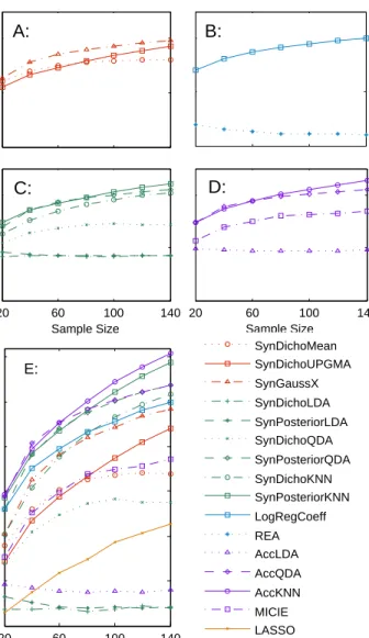
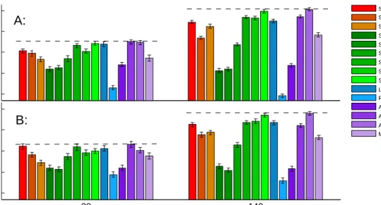
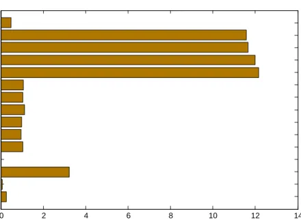
with the outcomeyin our simulated datasets (Exaggerated) coded by different shapes. 31 Figure 6 Simulation dataset results. . . 32 Figure 7 Simulation dataset results with20and140samples. . . 33 Figure 8 Run time comparison of all methods using simulated datasets. . . 35 Figure 9 Run time comparison of all methods of this chapter for different sample sizes using
simulated datasets. . . 36 Figure 10 Performance comparison between individual-based and network-based ranking for 20
simulated datasets in which we have weak individual effects and significant synergistic
effects. . . 43 Figure 11 Performance comparison between individual-based and network-based ranking for 20
simulated datasets in which we have both significant individual effects and significant
synergistic effects. . . 43 Figure 12 The AUC for predicting breast cancer metastasis based on network-based ranking and
individual-based ranking. . . 45 Figure 13 Venn diagram illustrating the identified biomarkers using different methods. . . 49 Figure 14 The pairwise distances between504Breast Cancer tumors are depicted with a gray scale
map (the distance values are quantile normalized to a normal distribution to achieve
Figure 15 Tumor stratification by finding densely connected sub-bipartite-graphs (relaxed bi-cliques) in a bipartite graph representation of the data which are constrained by prior
knowledge in the gene-gene interaction network. . . 58 Figure 16 Performance comparison with Ovarian cancer by survival analysis. . . 69 Figure A.17 Simulation dataset results with200randomly simulated variables in each sample. . 91
Abstract
In a modern systematic view of biology, cell functions arise from the interaction between molecular components. One of the challenging problems in systems biology with high-throughput measurements is discovering the important components involved in the development and progression of complex diseases, which may serve as biomarkers for accurate predictive modeling and as targets for therapeutic purposes. Due to the non-linearity and heterogeneity of these complex diseases, traditional biomarker identification approaches have had limited success at finding clinically useful biomarkers. In this dissertation we pro-pose novel methods for biomarker identification that explicitly take into account the non-linearity and het-erogeneity of complex diseases. We first focus on the methods to deal with non-linearity by taking into account the interactions among features with respect to the disease outcome of interest. We then focus on the methods for finding disease subtypes with their subtype-specific biomarkers for heterogeneous diseases, where we show how prior biological knowledge and simultaneous disease stratification and personalized biomarker identification can help achieve better performance. We develop novel computational methods for more accurate and robust biomarker identification including methods for estimating the interactive effects, a network-based feature ranking algorithm that takes into account the interactive effects between biomarkers, different approaches for finding distances between somatic mutation profiles for better disease stratification using prior knowledge, and a network-regularized bi-clique finding algorithm for simultaneous subtype and biomarker identification. Our experimental results show that our proposed methods perform better than the state-of-the-art methods for both problems.
Chapter 1 Introduction
1.1 Background
Many of complex diseases such as cancer and diabetes are influenced by a combination of several ge-netic and environmental factors. One of the major challenges in modern biomedicine is to understand the biological processes that drive such complex diseases. To enable systematic study of complex biological processes in terms of interacting molecular components, the focus has been on discovering the important cellular components, including genes or proteins, that are involved in development and progression of com-plex diseases. These components can serve as biomarkers for better disease diagnosis and prognosis and as targets for therapeutic purposes. Furthermore, discovering these biomarkers can help understand aber-rant changes that cause the disease, and enables targeted therapeutic and personalized medicine strategies. However, screening and validation using biomedical experiments or clinical trials is costly and demands a lot of resources. With the ever-increasing high-throughput data from systematic profiling of thousands of patients for diverse genome-scale omics measurements, including mRNA expression, micro-RNA (miRNA) expression, DNA sequences, somatic mutation profiles, and DNA copy number [1], there is a pressing need to develop computational approaches that help in identifying important components or biomarkers related to a certain phenotype of interest, among tens of thousands of measurements [2, 3].
Living systems are non-linear with highly interacting cellular components and heterogeneous with highly different molecular activities among similar phenotypic states [4, 5, 6]. Many complex diseases, such as cancer and diabetes, are conjectured to have complicated underlying disease mechanisms, which are neither static nor manifest as a linear systems [4, 5, 7] and exhibit complex genotypic and phenotypic heterogeneity within patients diagnosed with the same disease [6, 8, 9, 10, 11]. Multiple candidate risk factors, either genetic or environmental, and their interactions have been considered to play critical roles in triggering and determining the development of diseases [4, 5, 7, 3]. Owing to these challenges blind data mining without specifically modeling possible non-linearity and heterogeneity in disease mechanisms may lead to
fruit-less efforts even with more and “bigger” biomedical data. Previous computational methods for biomarker identification that ignore the potential interactive effects among risk factors and the heterogeneity in dif-ferent disease stages and subtypes have had limited success in identifying clinically useful information, even though significant resources and efforts have been exerted to collect as “big” and complete as possible omics data, such as in many epigenetic studies [12]. In addition, other characteristics in typical biomed-ical data, such as high noise, small sample size, extreme dimension of measurements under investigation, and the intrinsic heterogeneity, impose challenges for computational methods for accurate and reproducible biomarker identification [13]. In this dissertation we discuss the specific challenges of computational ap-proaches for biomarker identification in dealing with such complex and heterogeneous diseases and propose novel approaches to address them.
1.2 Problem Statement
In this dissertation we specifically explore biomarker identification for complex diseases in two general situations. In the first problem, biomarkers are identified among high-dimensional profiled measurements by finding a subset that possess high predictive power on the disease outcome (Figure 1 (A)). This problem is typically formulated as a computational problem of feature selection by considering each measurement as a feature in machine learning problems. In the second problem, we look at a heterogeneous population of patients, where we are interested in identifying biomarkers among high-dimensional profiled measurements for different disease subtypes while the actual subtypes or the outcome of interest, that can guide biomarker identification, are unknown. This problem is commonly referred to as tumor stratification for personalized medicine, where unsupervised machine learning methods such as clustering and bi-clustering are usually used for finding subtypes, and subtype specific biomarkers (Figure 1 (B)).
In the following two sections we provide brief background on the above two problems (a thorough liter-ature review is provided in Chapter 2) and point out the main shortcomings of the existing computational methodologies that we address in this dissertation.
1.2.1 Biomarker Identification for Disease Outcome
Feature selection techniques have been used to identify disease biomarkers based on high-throughput biomedical data [2, 3]. Given a set ofp measured components as features fornsamples,Xn×p, together
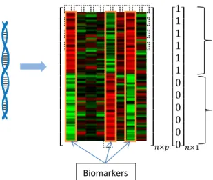
A: Biomarker identification for disease outcome (feature selection)
⬚ ⬚ ⬚ ⬚ ⬚ ⬚ ⬚ ⬚ ⬚ ⬚ ⬚ ⬚ ⬚ ⬚ ⬚ ⬚ ⬚ ⬚ ⬚ ⬚ ⬚ ⬚ ⬚ ⬚ ⬚ ⬚ ⬚ ⬚ ⬚ ⬚ ⬚ ⬚ ⬚ ⬚ ⬚ ⬚ ⬚ ⬚ ⬚ ⬚ ⬚ ⬚ ⬚ ⬚ 𝑛×𝑝 1 1 1 1 1 1 0 0 0 0 0 0 𝑛×1
Measurements (X) Outcome (Y)
Tu m o r s a m p le s DNA N o rm a l s a mples Biomarkers Clustering approach B: Biomarker identification for subtypes of a heterogeneous disease
Measurements (X) Bi-clustering approach ⬚ ⬚ ⬚ ⬚ ⬚ ⬚ ⬚ ⬚ ⬚ ⬚ ⬚ ⬚ ⬚ ⬚ ⬚ ⬚ ⬚ ⬚ ⬚ ⬚ ⬚ ⬚ ⬚ ⬚ ⬚ ⬚ ⬚ ⬚ ⬚ ⬚ ⬚ ⬚ ⬚ ⬚ ⬚ ⬚ ⬚ ⬚ ⬚ ⬚ ⬚ ⬚ ⬚ ⬚ 𝑛×𝑝
Bi-clusters (subtypes and their biomarkers)
A ll tu m o r s a m p les ⬚ ⬚ ⬚ ⬚ ⬚ ⬚ ⬚ ⬚ ⬚ ⬚ ⬚ ⬚ ⬚ ⬚ ⬚ ⬚ ⬚ ⬚ ⬚ ⬚ ⬚ ⬚ ⬚ ⬚ ⬚ ⬚ ⬚ ⬚ ⬚ ⬚ ⬚ ⬚ ⬚ ⬚ ⬚ ⬚ ⬚ ⬚ ⬚ ⬚ ⬚ ⬚ ⬚ ⬚ 𝑛×𝑝 Cluster (subtype) B io m ar ke r N o t a b io m ar ke r
Figure 1. An illustration of different computational approaches for biomarker identification. The color map is used to show imaginary gene expression levels: red representing high expression, green meaning low expression, and black for normal expression.
from thosepfeatures that can help build predictive diagnosis and prognosis models for the disease (Figure 1 (A)). Despite recent advances in feature selection techniques, most of the studies focus on univariate analysis of high-throughput biomedical data [14, 15, 16, 17, 18, 19, 20, 21, 3]. The individual power of the features are estimated and the features are filtered based on this score. Most of the advanced multivariate filter or wrapper feature selection techniques are ineffective in dealing with high-throughput biomedical which can be explained by:
• The high-dimensionality of biomedical data makes the multivariate analysis almost impossible due to the exponential growth of the number of subsets that need to be evaluated.
• The small sample size and noise in the data makes the statistics based on multiple features less reliable.
• The domain experts in biology prefer the analysis based on individual features because it is more intu-itive and easier to understand and interpret.
• And more importantly, exhaustive search approaches tend to find spurious features due to overfitting mainly because no prior assumption is made about the underlying model.
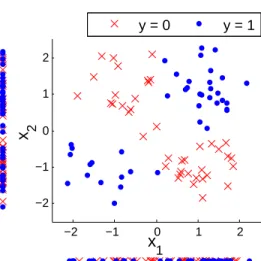
However, these analyses focusing on individual or marginal effects may not be sufficient as stated both in Genome Wide Association Studies (GWAS) [16, 18, 17] and in gene expression analysis [4, 5, 7] since two features with no significant individual effects can be highly “synergistic” and informative of the out-come when considered together [22] due to non-linearity as shown in Figure 2. Identifying such interactive effects among features not only helps identify more accurate biomarkers for outcome prediction, but also helps reveal functional interactions among cellular components which are specifically related to the pheno-type or outcome of interest [23, 22]. To overcome this problem with univariate analysis while avoiding the problems faced by previous multivariate feature selection, we can make a simplified assumption about the underlying model. Based on the nature of biological processes in cells we can assume that the components in cells (based on which the features are measured) regulate the biological processes either individually or by pairwise interactions with other components. This will enable more systematic analysis of biomedical data related to complex disease and more biologically interpretable feature selection as opposed to exhaus-tive search approaches. Feature selection based on this framework can be accomplished by measuring the individual effects and pairwise interactive effects between features and then filtering the features based on both scores. To find biomarkers considering interactive effects, most of the existing approaches first focus on detecting or measuring interactive effects among all the features and then use simple greedy approaches
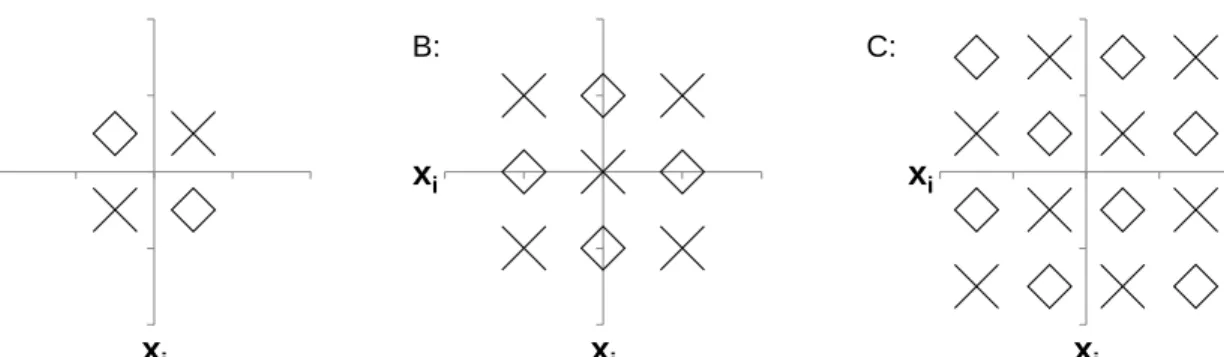
−2 −1 0 1 2 −2 −1 0 1 2 x1 x 2 y = 0 y = 1
Figure 2. An illustration of high interactive effect between two features x1 and x2 with respect to the
outcomey. The feauresx1 andx2are not able to discriminate the outcomeyindividually.
based on the ranked list of the pairs to select biomarkers [5, 4]. The performance of these methods is highly dependent on the accurate and robust measurement of interactive effects among features.
1.2.2 Biomarker Identification for Subtypes of Heterogeneous Diseases
There has been increasing evidence that many types of cancer are highly heterogeneous in the sense that associated somatic genes or other molecules may differ in different patients which usually results in different disease subtypes with varying behavior, including different survival time, different responses to drugs, and different recurrence rates [1, 8, 9, 10, 11, 6]. One of the important problems in cancer informatics is tumor stratification, where the goal is to find the tumor subtypes in a heterogeneous population of samples. In addition to finding relevant tumor subtypes, one other important problem is to identify the biomarkers (genes for example) related to each subtype for the purpose of personalized treatment and prognosis. Unlike supervised learning for previously proposed biomarker identification with respect to disease outcome, here the aim is to find biomarkers that better discriminate the disease subtypes in an unsupervised manner where the outcome or subtypes are not known.
There are two general computational approaches for identifying features (genes) associated with each subtype as biomarkers: (1) Clustering methods can be used to first stratify the tumor samples into subtypes and then for each subtype the genes that show significantly different values compared to other subtypes can be selected as the biomarkers. Here, identifying accurate subtypes is a crucial first step towards identifying
meaningful personalized biomarkers associated with heterogeneous diseases. (2) Bi-clustering approaches can be used to simultaneously find the subtypes and their corresponding biomarkers. The benefit of using bi-clustering approaches is that the bi-clustering methods may fail to find the correct clusters as they are utilizing all the genes for clustering, not specifically the relevant genes; and they may also fail to find the relevant genes after clustering as the performance depends on those clusters which may not be correct in the first place.
Using “big” data provided by high-throughput omics profiling techniques, researchers have used standard unsupervised clustering [1, 8, 9, 10, 11, 6] and bi-clustering approaches [24, 25, 26] to find subtypes with significantly different survival rates, tumor stages or grades, histological types, and drug responses mostly based on mRNA expression profiles [1, 8, 9, 10, 11]. However, these methods have limited performance because usually the datasets contain a very small number of samples and the gene expression measurements are often noisy. A relatively more promising and less noisy source of biomedical data is the somatic mutation profiles [1], where each gene is represented by a binary vector of mutation profiles. However, the problem with mutation profiles is that the number of mutations for each tumor is usually very small compared to the total number of genes under investigation and the tumors rarely share the same mutations, due to the extreme heterogeneity of the disease. It is in fact very common for two clinically identical tumors to share only one mutation [1, 27]. Owing to these properties it is very difficult to compare the tumors by calculating the distance or similarity between mutation profiles [6]. Due to these critical issues traditional clustering approaches usually fail in achieving meaningful subtypes by simply clustering the mutation profiles. Fur-thermore, in traditional bi-clustering [24, 25, 26] the goal is to simultaneously cluster both rows (tumors) and columns (genes) of data matrix by finding sub-matrices (or so called bi-clusters) in which the subset of tumors behave similarly over the subset of genes. However, for binary somatic mutation matrix data (or the smoothed somatic mutation data in which the mutation signals are smoothed), we are only interested in bi-clusters (or sub-matrices) containing mostly1s (or large values). In other words, although a sub-matrix containing all zeros (or small values) is considered as a perfect bi-cluster in bi-clustering approaches, it does not indicate a meaningful subtype.
1.3 Our Contribution
In this dissertation we focus on addressing the main shortcomings of the existing computational method-ologies for the aforementioned two main problems.
For the first problem, we focus on the problem of estimating the interactive effect between features, specially focusing on finding methods for better estimation for continuous random variables (numerical features) when we have a limited number of samples. Based on the estimated interactive effects, we further propose a novel feature ranking approach based on a constructed synergy network [22] that takes into account interactive effects among features in addition to their individual effects.
For the second problem, we first focus on clustering somatic mutations and explore new ways of incor-porating biological knowledge to better estimate the distance between binary somatic mutation profiles. We show that information from GO annotations (please refer to Chapter 5) and other curated gene-sets such as pathway databases can help achieve better stratification for Breast Cancer. The benefit of this approach, as opposed to using gene-gene interaction network, is that we directly use separate gene-sets or modules instead of using the network as whole. We then focus on simultaneous identification of both subtypes and their corresponding biomarkers based on somatic mutation profiles, by solving a novel bi-clique finding problem in a bipartite graph.
1.4 Organization
The rest of this dissertation is organized as follows. In Chapter 2, we provide technical background on recent related computational methods used for biomarker identification and tumor stratification in the field of bioinformatics. Then in next two chapters we focus on the problem of considering interactive effects in biomarker identification. In Chapter 3, we first review previously proposed methods for interactive effect estimation. We then propose new approaches, along with a discussion of the problems and challenges in pre-vious methods and explain how these new approaches can address them. We then evaluate the performance of the interactive effect estimation methods on simulation experiments and compare their power in detect-ing actual interactions among simulated random variables (as features) with data of different sample sizes from small to large. The results show that our proposed new methods can detect interactive effects more accurately than other methods with both large and small sample sizes. Based on these estimated interactive effects, we further propose a novel feature ranking in Chapter 4, that takes into account interactive effects among features in addition to their individual effects to rank the features. We first test the performance of our network-based feature ranking method based on simulated datasets. We then show that it can help in finding more accurate biomarkers for prediction of breast cancer metastasis and type 1 diabetes compared to tradi-tional individual-based ranking approaches. We further show that the identified biomarkers, by considering
interactive effects, contain genes that are involved in important pathways related to cancer metastasis. Then in two chapters, we focus on biomarker identification for heterogeneous diseases. In Chapter 5, we focus on separate subtype identification and biomarker identification approaches. We propose novel methods for calculating the distance between somatic mutation profiles. We propose the use of prior biological knowl-edge in pathway databases and GO Annotations to address the non-linearity in disease and heterogeneity of the mutation profiles which can help achieve more accurate clustering for somatic mutation profiles. Fur-thermore, we discuss the problems in calculating the distance between sparse binary vectors and suggest a method to alleviate that. We show that our approach based on pathways and GO terms can perform bet-ter than the traditional clusbet-tering methods as well as the recent state-of-the-art NBS method in identifying actual subtypes of Breast Cancer using somatic mutation profiles. In Chapter 6, we propose a novel bi-clique finding method for simultaneous tumor stratification and biomarker identification based on somatic mutation profiles. We propose a novel formulation for bi-clique finding which can help take into account prior biological knowledge in the gene-gene interaction network to alleviate the noise and small sample size problem in biomedical data. And finally, in Chapter 7 we summarize the dissertation and provide possible new directions for research in the computational biomarker identification area.
Chapter 2 Literature Review
In this chapter, we provide a summary of related computational work in biomarker identification. We first discuss the recent feature selection approaches used for biomarker identification based on high-throughput biomedical data. We then review recent clustering and bi-clustering methods used for subtype and biomarker identification for heterogeneous diseases.
2.1 Feature Selection for High Throughput Biomedical Data
Feature selection has been studied in data mining and machine learning literature [28, 29, 3]. The feature selection techniques are usually organized in two main categories: filter methods and wrapper methods. In filtering techniques, the relevance of the features are measured by looking at the statistical association be-tween the features (or a subset of features) and the outcome. A score is calculated for each feature or subset and then the high scoring features or subsets of features are selected. Filter techniques are usually simple and fast, as they are independent of the classification algorithm. However, most of the filtering methods are univariate and focus only on the individual power of the features and ignore the possible interactions between features that might be informative of the outcome. To overcome this problem, a number of multi-variate analysis methods have been proposed to try to incorporate the interaction between features such as Correlation-based feature selection [28] and Markov blanket filter [29]. The wrapper techniques [30] are usually multivariate and search for a subset of features that provides the best classification accuracy for a given classifier. Several subsets of features are generated and evaluated by learning a classifier and esti-mating the empirical error rate. The wrapper methods take into account the specific classifier for feature selection and therefore provide more relevant features to achieve more accurate classifiers. However, they are very computationally intensive and they suffer from overfitting.
Despite recent advances in feature selection techniques, most of the studies in biomarker identification focus on univariate analysis of high-throughput biomedical data [14, 15, 16, 17, 18, 19, 20, 21, 3]. The
indi-vidual power of the the features are estimated and the features are filtered based on this score. Most of the ad-vanced multivariate feature selection techniques are ineffective in dealing with high-throughput biomedical due to high-dimentionality of biomedical data, small sample size problem, lack of biological interpretabil-ity, and no effective prior assumption about the underlying model, as discussed in Section 1.2.1 of Chapter 1. However, these analyses focusing on the individual effects may not be sufficient [16, 18, 17, 4, 5, 7] since two features with no significant individual effects can be highly “synergistic” and informative of the outcome when considered together [22] (Figure 2 of Chapter 1). For example, in [31], a study was done to discover multivariate logical predictive relations among gene expressions. They have found several XOR relationships similar to what is shown in Figure 2. For example, they showed that if both Interleukin18 and MRC1 genes are up-regulated or if both are down-regulated, then the EHHADH gene is down-regulated.
As explained in Section 1.2.1 of Chapter 1, to overcome this problem with univariate analysis while avoiding the problems faced by previous multivariate feature selection, we can make a simplified assump-tion about the underlying model. Based on the nature of biological processes in cells we can assume that the components in a cell (based on which the features are measured) regulate the biological processes either individually or by pairwise interactions with other components in the cell. Therefore, the cell can be viewed as individual components and pairwise interaction among them. This will enable a more systematic analysis of biomedical data related to complex disease and more biologically interpretable feature selection as op-posed to exhaustive search approaches. Feature selection based on this framework can be accomplished by measuring the individual effect and pairwise interactive effects between features and filtering the features based on both scores.
Several methods have been proposed both in GWAS [16, 18, 17] and other -omic data analyses [4, 5, 7] to take into account interactive effects among features. However, the performance of these methods highly depends on accurate and reliable interactive effect estimation, which is very difficult to achieve compared to individual effect, due to the small sample size problem in biomedical data. Recently, re-searchers have proposed different statistical and computational methods for measuring the interactive effect [32, 16, 17, 18, 33, 34, 23, 22, 4, 5, 35]. However, most of these proposed methods are designed for quan-tized or discrete random variables (nominal features) [16, 17, 18, 33, 32, 34, 35, 23] or have made simplified data distribution assumptions [32].
For better readability of the dissertation, we leave a more detailed literature review on methods for estimat-ing and incorporatestimat-ing interactive effects to Chapter 3, where we propose new methods for better interactive
effect estimation and compare the performance of all methods. We further propose a novel feature ranking in Chapter 4 that integrates both individual and interactive effects to sort the features.
2.2 Clustering Methods for Tumor Stratification
Using the data provided by high-throughput omics profiling techniques, researchers have used standard unsupervised clustering such as hierarchical clustering and Non-negative Matrix Factorization (NMF) to cluster the samples as subtypes [1, 8, 9, 10, 11, 6] to find subtypes with significantly different survival rates, tumor stages or grades, histological types, and drug responses mostly based on mRNA expression profiles [1, 8, 9, 10, 11].
In this section we summarize clustering approaches recently used for identifying subtypes in complex disease based on high-throughput biomedical data.
The traditional k-means clustering [36] is used by [37] to stratify tumor gene expression profiles. For a specified number of clusters K, k-means clusters the data into K groups such that following objective function is minimized E= K X i=1 X O∈Ci |O−µi|2
whereO is a data point andCi is the set of all data points categorized in theith group andµi is the cluster
centroid or the mean of the data points in Ci. To optimize the above objective function, k-means uses a
two step procedure: first each data point is assigned to the closest cluster based on the distance from the centroids; in the second step the cluster centroids are updated based on the new data point assignments.
Hierarchical clustering is another traditional clustering method widely used for tumor stratification [8, 9, 10, 11]. Based on the distances between data points and between clusters, the hierarchical clustering generates a nested tree structure called dendrogram. The dendogram then can be cut at any level to obtaining any specified number of clusters. There are two ways of generating the tree: bottom-up (Agglomerative) approach in which initially each data point is considered as a separate cluster and, for example, in each further step the two closest clusters are merged until only one cluster remains; top-down (divisive) approach where initially all data points are put in one cluster and in each further step the large clusters are split, based on a certain criteria, until only singleton clusters remain. One widely used variation for clustering biomedical data is called UPGMA [38] where the distance between two clusters is calculated as the average distance between all pair of points across the two clusters.
Other model based clustering methods are also frequently used for clustering biomedical data [39]. In latent model based clustering, the data points are assumed to come from a mixture of distributions with each component representing one cluster. Assuming the probability density function for theith componentCiis
f(x, θi), the mixture model is
P(x=xr) = K
X
i=1
γr,if(x=xr, θi)
in whichK is he number of components and the hidden parameterγki is the mixture parameter indicating
the probability of therth data point coming from theicomponent. Due to the hidden variable involved in such mixture models, a two step algorithm, Expectation Maximization (EM) can be used to find the maxi-mum likelihood estimation of the parameters. One of the variations of these model based clustering is called the Gaussian Mixture Model in whichf(x)is assumed to follow the Gaussian distribution and is widely used for clustering gene expression profiles.
To achieve more robust clustering, consensus clustering [40] techniques are also extensively used for tu-mor stratification based on biomedical data [41, 1, 42, 43]. Consensus clustering is usually used to combine the results of several clustering methods based on different types of biomedical data [44] or to aggregate the clustering results based on several runs of clustering on a single dataset [6]. Several approaches has been proposed for combining the multiple clustering results [40]. For example, [40], proposed an approach to combine the clustering results of multiple runs of the same clustering algorithm on different sub-samplings of the dataset. They first generate a co-clustering matrixCCn×n (nis the number of samples), in which
CCi,jis equal to the number of timesith andjth datapoints are clustered together divided by the number of
times both appeared in a sub-sampled dataset. The resulting consensus matrix provides a similarity measure between datapoints which can be used in conjunction with agglomerative hierarchical clustering to generate a dendogram tree.
Matrix factorization techniques which are usually used to represent data in a lower dimension, can also be used for clustering proposes. Among them Non-negative Matrix Factorization (NMF) [45] is widely used for clustering gene expression profiles, however, a preprocessing step is always required to create a non-negative matrix from gene expression data. Given the non-negative representation of the dataXn×m
and and a pre-specified number of clustersK, the NMF algorithm finds two non-negative matricesWm×K
andHn×Kthat minimize the residual error||X−HWT||F2. The columns ofW are usually called the
meta-genes (a combination ofmgenes) representing the clusters and each row ofHcontainsKvalues indicating the probability of the data-points belonging to each one of theK clusters. The maximum value in theith
row ofHindicates the cluster to which theith element is assigned. To solve this optimization problem mul-tiplicative updating rules are used that converge to the local minimum of the above optimization problem [45]: Hik ←Hik (XW)ik (HWTW) ik Wik ←Wik (XTH)ik (W HTH) ik
Most of the traditional clustering approaches are suitable for gene expression, however, as previously shown [6], these methods have limited performance because usually the datasets contain a very small num-ber of samples and the measurements are often noisy. A relatively more promising and less noisy source of biomedical data is somatic mutation profiles, where each tumor is represented by a binary vector of muta-tion profiles. However, clustering binary mutamuta-tion profiles is difficult due to their extreme sparseness and heterogeneity. To address this issue [6] proposed a network-based stratification (NBS) framework that takes advantage of two sources of information to find subtypes: 0-1matrixAn×mcontaining the somatic
muta-tion profiles ofmgenes fornpatients; and the adjacency matrixMm×mof a gene-gene interaction network.
They first smooth the mutations inAover the networkMusing a network propagation technique introduced in [46] using the following recursive formula:
At+1=αAtM0+ (1−α)A0 (2.1)
whereA0is equal to somatic mutation matrixA,M0is obtained by dividing each column ofMby the
sum-mation of elements in that column (degree normalized adjacency matrix). The tuning parameterαcontrols the distance in which mutation signal is allowed to diffuse into the network. The propagation spreads the influence of the mutation to the neighboring genes in the network. The new smoothed somatic mutation matrix is then decomposed using Network-regularized NMF originally proposed by [47] by minimizing the following objective function:
min
W,H>0||A∞−HW
T||2+trace(W LWt)
MatricesHn×KandWm×Kform a decomposition of the network smoothed matrixA∞n×m, whereKis the
ofH are the weighted cluster assignments to each one ofK clusters where the largest value on each row indicates the assigned cluster to the corresponding patient tumor. The matrix L is the Laplacian matrix computed based on the adjacency graphM. By minimizing the term trace(W LWt), the basis vectors in W are constrained to respect local network neighborhoods, i.e., connected genes in the network tend to have similar corresponding values in basis vectors. Similar to NMF, following multiplicative updating rules derived for Network-regularized NMF [47]:
Hik ←Hik(HW(XWTW)ik) ik Wik ←Wik (X TH+M W) ik (W HTH+DW) ik
in which,Dis the diagonal matrix of the degrees of nodes in the network corresponding toM. The above multiplicative updating rules are proved to converge to local minimum of the above optimization problem [47].
2.3 Bi-clustering Methods for Simultaneous Tumor Stratification and Biomarker Identification
One traditional approach for for simultaneous subtype and biomarker identification is bi-clustering [24, 25, 26] where the goal is to simultaneously cluster both rows (tumors) and columns (genes) of a data matrix by finding sub-matrices (or so called bi-clusters) in which the subset of tumors behave similarly over the subset of genes. Based on the application of interest several definitions exist for bi-clusters. For example, constant bi-clusters are the sub-matrices of data with almost the same values. Other bi-clustering approaches may look for sub-matrices with constant values on rows or on columns. Several surveys on different types of bi-clusters and the algorithms to find them are provided in [24, 48, 49]. In traditional bi-clustering approaches, usually a measure of quality for bi-clusters, e.g. mean squared residue(MSR) or scalling mean squared residue (SMSR), are defined and heuristic algorithms are used to find bi-clusters with high quality [50, 51]. Here we review recent more sophisticated bi-clustering approaches used for analyzing biomedical data [52, 53, 54, 55].
Several probabilistic modeling approaches are used for bi-clustering [52, 53]. In [52] they proposed a probabilistic modeling approach called Plaid Models (PM) for multivariate analysis of gene expression data. They assume that the data matrix is an image generated by different layers representing the underlying bi-clusters with different colors. Based on this, they assume following model for the gene expression values
in the gene expression data matrixY: Yij =µ0+ K X k=0 µkδikκjk
in whichK is the number of desired bi-clusters,µ0 is the background color,µk is the main effect (color)
of thekth bi-cluster,δikandκjk are binary values indicating whether theith gene andjth sample belong to
cluster. This model can be used to find constant bi-clusters. To further improve the model, [53] proposed a Bayesian approach, called the Bayesian Biclustering model (BBC), that allows multiple bi-clusters without overlapping samples or overlapping genes. They assume the following model:
Yij = K X k=1 ((µk+αik+βjk+ijk)δikκjk) +eij(1− K X k=1 )δikκjk,
whereαik andβjk are the effect of sampleiand genej which are added to allow finding bi-clusters with
constant rows and constant columns,ijk is the noise term for clusterk, andeij is used to model the data
points that do not belong to any clusters. The priors of the indicatorsκ andδ are set as follows to avoid overlapping samples in bi-clusters:
κij ∼Bernoulli(qk)
P(δij = 1, δil= 0, l6=k) =pk
P(δil = 0, l= 1,2, ..., K) =p0 = 1−PKk=1pk
wherepkandqkare constant. The following a priori assumptions are made:
µk ∼N(0, σµ2k) αik|δik= 1 ∼N(0, σα2k) βik|κik= 1 ∼N(0, σ2βk) ijk ∼N(0, σ2k) eij ∼N(0, σe2) (2.2)
where all theσ2 are assumed to follow an inverse Gamma distribution. To learn the model they use a Gibbs sampling method. Further improvement over the above method is provided in [55]. They provide a Bayesian Framework for bi-clustering called the Penalized Plaid Model (PPM), in which they propose a method to find the optimal number of bi-clusters and address overlapping. In this model, the hard-EM algorithm has been used for parameter estimation. Another probablistic bi-clustering approach is cMonkey [54]. Recently, [25] used cMonkey for stratification of breast cancer tumors, which shows promising results in identifying phenotipically heterogeneous subtypes together with their corresponding biomarker or feature set.
Other approaches for bi-clustering propose the use of Matrix Factorization methods to find the bi-clusters. One famous algorithm called Non-smooth Non-negative Matrix Factorization (nsNMF) [56] is used in [57] to analyze gene expression profiles. This algorithm is motivated by the NMF clustering algorithm explained previously in this section but provides very sparse matrices and therefore enables gene selection for identified subtypes. They propose to approximate data matrixXn,mbyW SHwhereW andHare the same as in the
original NMF method. The positive symmetric matrixSK×K, is called the smoothing matrix defined as
S= (1−θ)I+ θ
K11
T,
where IK×K is the identity matrix and 1 is a vector of lengthK with all the elements equal to 1. The
parameterθis the ”smoothness” parameter that controls the sparseness of the of the final solution. To find the solution, they propose an algorithm to minimize the divergence ofXfromW SH defined as follows:
D(X, W SH) = n X i=1 m X j=1 Xijln Xij (W SH)ij −Xij+ (W SH)ij .
They further provide an iterative algorithm based on the following rules to findW andHthat minimizes the divergence. Hik ← Hik Pn j=1((W S)jk(X)ij)/PKq=1((W S)jq(H)qi) Pn j=1(W S)jk Wik ← Wik Pm j=1((HS)kj(X)ij)/PKq=1((W)jq(HS)qj) Pn j=1(HS)jk Wik ← Wik Pn j=1(W)jk
All of the above discussed approaches for bi-clustering are designed for analysis of gene expression pro-files which are real valued vectors. As discussed in the introduction, the tumor stratification problem using somatic mutation data can be better represented as finding densely connected sub-graphs in a bipartite graph, which enables both subtype identification and personalized biomarker identification for each subtype. More formally, given the somatic mutation data matrixAn×p, which contains the smoothed somatic mutation
pro-files ofpgenes forntumors, we can construct its corresponding bipartite graph denoted byG= (U, V, E)
, where the node setU = {u1, ..., un}is in one part of the graph representing the tumor samples, and the
node setV ={v1, ..., vm}is in the other part of the graph representing the genes. Nodeviis connected to
uj with weightAi,j ifAi,j >0.
Community detection and graph partitioning approaches have been studied for finding densely connected subgraphs [58]. In community detection or graph partitioning, the nodes in a given graph are clustered in an arbitrary number of partitions, modules, or communities such that the clusters are highly connected internally while there are a small number of connections across different clusters. Although these methods can be used to find clusters in any graph, recently, researchers have proposed alternative methods that per-form better for bipartite graphs [59, 60, 61]. In the following, we discuss two methods for bipartite graph clustering proposed by [61, 59] that can be used for tumor stratification.
One approach for finding densely connected subgraphs is a graph partitioning approach in which the aim is to divide the graph nodes into two groups such that the number of edges between groups or the cut is minimum [60, 61]. In [61] they propose a method for partitioning the bipartite graph by minimizing the ratio-cut between the partitions. For a graphG= (V, E)(|V|=n), the ratio-cut between two partitionsV1
andV2(V1∪V2 =V andV1∩V2=∅) is defined as:
Ratio-cut= cut(V1, V2)
|V1| +
cut(V1, V2)
|V2| .
They show that solving the following optimization problem finds the partitions that minimize the Ratio-cut:
min q6=0
qTLq
qTDq, subject toq
TDe= 0
whereqof sizenis a{−1,1}assignment vector (qi = 1meansith node in the graph is assigned to first partition andqi =−1meansith node in the graph is assigned to second partition),Dis a diagonal matrix of node degrees,Lis the Laplacian matrix ofG, ande= [1, ...,1]T. This problem is also NP-complete so
they propose a spectral graph algorithm in which they relax the values of the elements inqto take any real number. They prove that a solutionq∗ of the relaxed problem is equal to the eigenvector corresponding to the second smallest eigenvalue of the following generalized eigen system problem:
Lz=λDz
To find larger numbers of partitions they suggest either calling the spectral partitioning problem recursively or using other eigenvectors of the above problem to form a matrixZ and perform k-means clustering algo-rithm. For the case of a bipartite graph with adjacency matrixAn×m, they defineAn =D
1 2 1AD 1 2 2 in which
D1 and D2 are diagonal matrices of degrees for the left part of the bipartite graph and right part of the
bipartite graph respectively. They then prove that the solution for the bipartite partitioning problem are the left and right singular vectors corresponding to the the second smallest singular values ofAn.
Another approach for community detection was proposed by [62], in which they used the leading eigen-vectors of a Modularity matrix of the graph to find the communities. This method is further extended for bipartite graphs in [59], in which they define a modularity matrix suitable for bipartite graphs and use the left and right singular vectors of the new modularity matrix to find the clusters. Given the adjacency matrix An×mof a bipartite graph, they define the modularity matrixB asB =A−P wherePij = kmidj,ki is the
degree of theith node inU, anddjis the degree of thejth node inV. The module or community assignment
of the nodes inUandV can be represented by assignment matricesSn,K andGm,K whereKis the number
of communities or modules,Si,k = 1if theith node inU belongs tokth module, andGj,k = 1if thejth
node inV belongs tokth module. The modularityQof a given assignmentsSandGis defined as
Q= 1
mtrace(S
TBG)
Now the problem is to find the assignment matricesS∗ andG∗ that maximize the modularityQwhich is computationally intractable. Instead, they use singular vector decomposition to find the left and right leading singular vectors ofBto obtain approximate solutions for the corresponding relaxed problems.
Neither of the above graph partitioning and community detection methods have been tested for the strat-ification problem, but it has shown promising results in finding community groups in bipartite social net-works [59] and document clustering [61]. However, these methods may not be appropriate for stratification
problems as they attempt to cluster all the genes, while in stratification we are interested in finding a few important genes or biomarkers for each identified subtype and the rest of the genes could be put aside.
The most dense subgraphs in bipartite graphs are bi-cliques. The problem of finding and enumerating all edge maximal bi-cliques has been studied in literature [63, 64, 65, 66] among which [64] proposed a novel approach to efficiently find large bi-cliques. LetAn×m be the adjacency matrix of the bipartite graphG, a
maximal bi-clique can be computed by finding solution of the the following optimization problem:
maxs,gsTAg s.t. si>0fori∈ {1..n} gi >0fori∈ {1..m} Pn i=1sαi = 1 Pm i=1g β i = 1
Given a solution (s∗,g∗) of the above optimization problem, the nodes in left part and right part of the maximal bi-clique are indicated by non-zero elements ins∗andg∗respectively. The parameters1< α≤2
and1< β≤2favor different shapes of cliques: If for exampleα > βthen it tends to find the cliques with a larger number of nodes from the left side than from the right side. Also, settingα, β to a value close to
1(e.g. 1.05or1.1) helps find very tight (exact) cliques and setting α, β to larger values (e.g. 1.2) could find loose cliques with some missing edges. The latter is more useful in most of the applications such as tumor stratification since densely connected subgraphs are more realistic. To solve the above optimization problem, they use following multiplicative update rules:
s(it+1) = s(it) (Ag (t)) i [s(t)]TAg(t) 1/α gi(t+1) = gi(t) (A Ts(t)) i [s(t)]TAg(t) 1/β
Starting from a random feasible s0 and g0 they prove that the multiplicative update rules converge to a
point satisfying KKT conditions for local maxima. To find multiple bi-cliques they suggest deleting the first bi-clique from the matrixAand performing the above algorithm to find the next bi-clique. This can be repeated until we find a desired number of bi-cliques. Unlike graph partitioning or community detection approaches, bi-clique finding is able to set aside irrelevant genes as it does not attempt to cluster all the
genes. It tends to find highly densely connected subgraphs which usually contain small numbers of genes. In Chapter 6, we will show how this method can be extended to incorporate knowledge from gene-gene interaction networks for better simultaneous tumor stratification and biomarker identification.
Chapter 3
Detecting Pairwise Interactive Effects For Continuous Random Variables
In this chapter, we first review the previously proposed methods for estimating the interactive effects between features focusing on the methods dealing with continuous random variables (In this chapter we assume that the features are continuous random variables and we will refer to them as variables). We then propose new methods for better estimation of interactive effects especially for the small sample size scenario. We represent biomedical data byXwhich is an-by-pmatrix, wherepis the number of candidate variables andnis the number of observations or samples. Typically in biomedical data we have:pn. Throughout this chapter we investigate methods for measuring the interactive effect between two continuous random variablesxi andxj with respect to the outcome variable y, which, for example, can be binary denoting
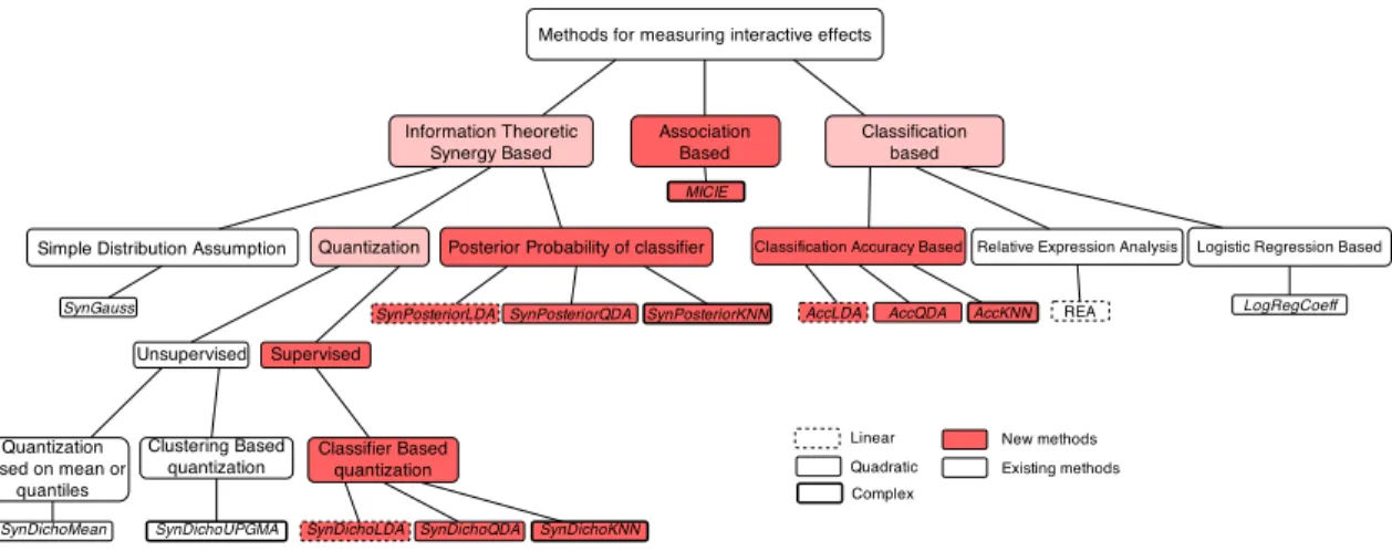
whether the corresponding samples come from “healthy” or “diseased” subjects. We review the previously proposed methods, especially focusing on the ones studying continuous random variables; and then further propose a set of new methods to better detect interactive effects. We have categorized existing methods together with our newly proposed methods into three categories: (1) Information theoretic synergy based methods [32, 22, 23], in which marginal and conditional probability distributions of xi, xj, and y are
estimated from data to compute the information theoretic synergy as interactive effect. In this category, the reliability of interactive effect estimation depends on how well the involved probability distributions are estimated; (2) Classification based methods [34, 5, 4], in which first a classification model is learned from the data and then the interactive effect is measured by some parameters in the model, such as coefficients in Logistic Regression, relative values of variables in Relative Expression Analysis (REA), or estimated synergistic predictive power of xi and xj to y using classification accuracy; and (3) Association based
methods, where the interactive effect is measured by the increase in association betweenxi andxj after
observing the outcomey. In Figure 3, we have laid out a hierarchy of the approaches studied in this chapter that include the existing methods as well as our newly proposed methods.
We evaluate the performance of all the methods based on simulations and compare their power in de-tecting underlying interactions among simulated random variables with data of different sample sizes. The
Figure 3. All the methods studied in this chapter with their relationships illustrated in a tree graph.
simulation results show that our proposed methods outperform many existing methods for interactive effect estimation in general.
3.1 Existing Methods
Here we review the existing methods in the literature for measuring interactive effects between two con-tinuous random variablesxiandxj on a categorical outcomey.
3.1.1 Information Theoretic Measures
One of information theoretic measures is based on the definition of synergy Syn(xi,xj;y)by
Anastas-siou et al. [23], which measures the portion of the information gain from the pair of covariates (xi,xj)
subtracting their individual information gain [67]:
Syn(xi,xj;y) =I(xi,xj;y)−I(xi;y)−I(xj;y), (3.1)
whereI(x;y) =H(y)−H(y|x) =H(x)−H(x|y)can be considered as the amount of the information gain measured in the reduction of the entropy ofyafter knowing the value of either individual or multiple variables. Hence, it is essential to accurately estimateI(x;y), which can be challenging under the small sample size scenario withpn. Further expanding the formula in (3.1), we can rewrite the synergy based
on conditional entropies: Syn(xi,xj;y) = H(xi,xj)−H(xi,xj|y) +H(xi|y)−H(xi) +H(xj|y)−
H(xj) = H(y|xi) + H(y|xj)−H(y|xi,xj) −H(y). For quantized random variables x and y, we
can have relatively reliable maximum likelihood estimates of conditional entropiesH(y|x) =P
µP(x=
µ)P
ν−P(y = ν|x = µ) log(P(y = ν|x = µ))if the sample size is reasonably large [23, 35, 33, 32].
When x is continuous and y is discrete, we can compute conditional entropies H(x|y) = P
νP(y = ν) +∞ R −∞ −P(x = µ|y = ν) log(P(x = µ|y = ν)))dµ; and H(y|x) = +∞ R −∞ P(x = µ) Pν−P(y =
ν|x =µ) log(P(y = ν|x = µ))dµ. Clearly, in this case, it is more difficult to have reliable conditional entropy estimates, especially with the limited sample size, which is often the case in biomedical research. We now first review the existing methods that estimate conditional entropies for continuous input variables with binary outcome.
3.1.1.1 Quantization Methods
The first intuitive approach for continuous random variables is to quantize the data and estimate the conditional entropies as quantized random variables. Generally, the observed values of continuous random variables can be categorized into several groups for quantization. The obtained quantized variablexcwill be
used to compute the conditional entropyH(y|xc)as an approximate estimate forH(y|x)and consequently to estimate Syn(xi,xj;y).
One simple quantization scheme is to take the corresponding sample mean estimates mi = n1 Pn`=1x`i
as the threshold to dichotomize the original measurements as Bernoulli random variables. There are other quantization schema. For example, instead of using mean values, we can quantize by quantiles. Also, to estimateH(y|xi,xj), the quantization of the pair of variables can be done simultaneously. For example,
one can categorize the observed values ofxi andxj into two groups by using the line xi−xj = 0as a
separating line which categorizes the data points in the(xi,xj)plane into two groups: The sample points
withxi ≥ xj and the points with xi < xj, which indeed is the essence of Relative Expression Analysis
(REA) [5].
The main problem with those quantization methods is that the appropriate thresholds or separating cri-teria for quantization are generally unknown. More complicated clustering methods have been proposed for automatic quantization. For example, Anastassiouet al. [22] have proposed an UPGMA hierarchical clustering method to quantize continuous variables. By taking clustering results at different levels of the hierarchy, the average estimates of conditional entropies with different numbers of clusters are used as the
robust interactive effect estimates [22]. Other clustering methods (e.g. in [68]) can be used for more compli-cated quantization of continuous variables. We will test the performance of the following specific methods in this category:
• SynDichoMean: dichotomize by sample mean estimates.
• SynDichoUPGMA: quantize by the UPGMA clustering [22]. Implementation details can be found in Section1ofAppendix A.
3.1.1.2 Simplified Gaussian Assumptions
Instead of quantization, we can also estimate conditional entropies by assuming that input variables fol-low simple distributions as done in [32]. For example, assuming thatxfollows a Gaussian distribution (a multivariate Gaussian distribution ifxdenotes multiple variables), we can obtain the corresponding maxi-mum likelihood estimates (MLE) of the distribution parameters, the expectation and standard deviation in this case. Given the standard deviationσ (or the covariance matrixΣ), the entropyH(x) can be directly computed as 12ln(2πeσ2) (or 12ln|2πeΣ|for multivariate cases). Based on this, we can then estimate the synergy Syn(xi,xj;y). In our simulation experiments, we will test its performance and refer to this method
asSynGaussX.
3.1.2 Classification-based Methods 3.1.2.1 Logistic Regression
The most commonly used statistical model for relating input variables x and a given binary outcome y is arguably the logistic regression model [69], in which the effect of a variable on the outcome can be measured by its corresponding model coefficient after fitting with the given data. Based on this, the interactive effect of two variablesxiandxj on the outcomeycan be computed similar to individual effect
by−log(p)wherepis the p-value of the coefficientβ after fitting the following logistic regression model
log(g/(1−g)) = α0+α1xi +α2xj+βxixj, in whichg =p(y = 1|xi,xj)[34]. We later refer to this
method asLogRegCoeff in our simulation experiments and we note thatLogRegCoeff is a quadratic method due to the integration of the interaction terms.
3.1.2.2 Relative Expression Analysis
This method has been proposed by [5] to find interactive pairs of genes based on their relative expression. Given two input variablesxi andxj, the interactive effect associated with the outcomeycan be measured
by IE=|P(xi <xj|y= 0)−P(xi<xj|y= 1)|. The estimate forP(xi <xj|y= 0)is the frequency of
the observations withxi <xj andy= 0and similarlyP(xi <xj|y= 1)is the frequency of observations
withxi < xj andy = 1by MLE. Looking deep into their method reveals that they have used the linear
functionxi=xj to quantize data points in the two-dimensional plane(xi,xj)and assumed that this line is
a proper quantization boundary. Based on this assumption, they expect that for highly interactive pairs, the linexi =xjbetter discriminates samples with larger IE. We also evaluate its power of detecting interactions
in our experiments and refer to this method asREA.
3.1.2.3 Linear Classifiers
For highly interactive pairs of variables, it is intuitive to expect that we can train simple classifiers that possess certain discriminating power. Based on this, a procedure based on permutation tests has been pro-posed in [4] to test each pair of input variables xi,xj to find significantly interacting pairs by estimated
classification accuracies based on Linear Discriminant Analysis (LDA). They perform two empirical signif-icance tests: the first to rank variable pairs by estimated accuracies and the second to check whether this accuracy is only due to interactive effects of variables by permuting one variable in each pair. Based on these tests, highly ranked pairs were considered significantly interacting pairs. However, the procedure depends on the relative difference of estimated accuracies and does not provide a measure for evaluating interactive effects. Motivated by this procedure, we propose new interactive effect estimates based on the classification performance in the following sections.
3.2 Our Proposed Methods
3.2.1 New Information Theoretic Measures
In this section, we first propose two new methods to estimate information theoretic synergy for continuous random variables based on supervised modeling.
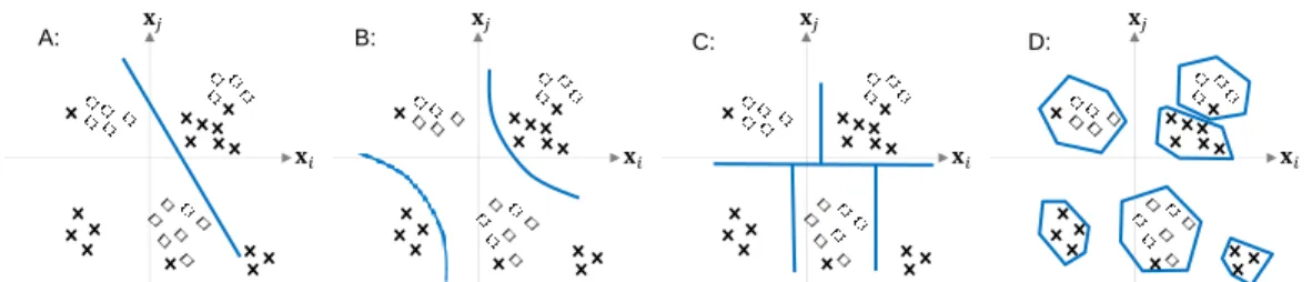
𝐱𝑗 𝐱𝑖 𝐱𝑗 𝐱𝑖 𝐱𝑗 𝐱𝑖 𝐱𝑗 𝐱𝑖 A: B: C: D:
Figure 4. Illustration for how different quantization methods work. A: Linear separating boundary. B: Quadratic separating boundary. C: UPGMA clustering based separating boundary. D: KNN based separating boundary.
3.2.1.1 Supervised Quantization
Previous information theoretic measures are done in an unsupervised fashion in the sense that either quantization or distribution assumptions ofxare made without consideringy. Hence, it may lose critical predictive information as the approximation by quantization may destroy the underlying structure of data. We explore new supervised quantization for better estimates of interactive effects by taking into account the information given in y. More specifically, we propose new supervised quantization approaches based on existing classification methods at different levels of complexity, in which we search for the best possible separating boundaries detected by a classification algorithm for quantization. In other words by learning a classifier, all the possible separating boundaries based on the type of classifiers e.g. line (linear classifier), hyperbola (quadratic classifier), and Voronoi diagram (KNN classifier) can be explored. The separating boundary which minimizes the error is assumed to be the most appropriate boundary for quantizingx. To accomplish this, we first learn a classifier to predictyfromx, and then for each observationx(`),1≤`≤n we predict its corresponding outputy(`) ∈ {0,1}by the learned classifier, which is considered as the new quantized value of x(`). Similar to previous information theoretic measures using quantization, we can
now estimate the probabilities and compute conditional entropies using quantized variable x. Note that depending on the classifier used, the separating boundaries may change. For example, simple modeling methods like LDA will find the best possible linear boundaries to categorize the data x while KNN (K Nearest Neighbor classifiers) can find more complex boundaries with increasing K but may overfit the data. An illustrative example of how different methods may quantize(xi,xj) is shown in Figure 4. We
expect that the integration of the outcome information and exploring non-linear interactions among variables can capture more general interactive relationships among variables than unsupervised linear ones like the previously discussed methods [22, 5, 4]. In order to test our hypothesis, we evaluate the performance of the following supervised quantization methods:
• SynDichoLDA: LDA classifier (MATLAB implementation) [70] is used to find a linear separating boundary to quantizex.
• SynDichoQDA: Quadratic Discriminant Analysis (QDA) classifier (MATLAB implementation) [70] is used to find a quadratic separating boundary to quantizex.
• SynDichoKNN: KNN classifier is used to find a non-linear separating boundary to quantizex. In order to avoid overfitting, we implement a method similar toSynDichoUPGMAand estimate interactive effects by averaging over multiple KNN classifiers with differentK. Implementation details can be found in Section2ofAppendix A.
3.2.1.2 EstimatingP(y|x)by Supervised Learning
In this section, we propose another new way to estimate conditional entropiesH(y|x)by directly estimat-ing theP(y|x)without quantization. Usually, classification methods are used to learn the relation between input variablesxand the outcomey. After learning the classifier, for any observationx(`),1≤`≤n, the classifier can predict its corresponding most probable outputy(`)∈ {0,1}. In addition, many classification methods, such as Naive Bayes, Logistic Regression, LDA, and QDA, can provide estimates of the posterior probabilitiesP(y|x=x(`)). For example, in LDA, to estimate the posterior probability, first the probabili-tiesP(y),P(x), andP(x|y)are estimated by assuming Bionomial and Gaussian distributions respectively, and the posterior probabilityP(y|x)is then computed using the Bayes rule:P(y|x) =P(x|y)P(y)/P(x). In other classifiers including Decision Trees, Support Vector Machines (SVM), and KNN, the posterior prob-abilityP(y=y(`)|x=x(`))for a given inputx(`)can be considered as a value describing how confident the classifier is ony(`). For example, in KNN, if from theK nearest neighbors ofx(`),tof them have class
label1, then we can approximately estimate that the posterior probabilityP(y= 1|x=x(`)) = Kt and the posterior probabilityP(y= 0|x=x(`)) = K−t
K . With these estimates ofP(y|x), we can always estimate
the conditional entropiesH(y|x)using following formula:
H(y|x) = +∞ Z −∞ P(x=x) X y∈{0,1} −P(y=y|x=x) log(P(y=y|x=x))dx. (3.2)
But the problem with the above formula is that we need to estimateP(x), for example, by making a Gaus-sian assumption or by quantization as discussed earlier. Such assumptions and approximations may lead to
inaccurate estimates of the desired conditional entropies. To overcome this problem, the empirical distribu-tion ofxbased on the givennobservations can be used:P(x=x) = n1Pn
`=1δ(x−x(`)), in whichδ(.)is
the Dirac Delta function. Substituting this empirical distribution ofP(x)into the equation (3.2) we get:
H(y|x) = +∞ Z −∞ 1 n n X `=1 δ(x−x(`)) X y∈{0,1} −P(y=y|x=x) log(P(y=y|x=x))dx. (3.3)
Taking the integral into summation we get
H(y|x) = 1 n n X `=1 +∞ Z −∞ δ(x−x(`)) X y∈{0,1} −P(y=y|x=x) log(P(y=y|x=x)) dx. (3.4)
Also, based on the definition of the Dirac Delta function, we have
+∞ R −∞ δ(x−α)f(x)dx = f(α), which implies that: H(y|x) = 1 n n X `=1 X y∈{0,1} −P(y=y|x=x(`)) log(P(y=y|x=x(`))).
Based on the above formula we can efficiently estimate H(y|x). In our simulation experiments, we test the performance of the following specific methods for measuring interactive effects based on the direct estimation ofP(y|x):
• SynPosteriorLDA: The posterior probability estimated by LDA (MATLAB implementation) [70].
• SynPosteriorQDA: The posterior probability by QDA (MATLAB implementation) [70].
• SynPosteriorKNN: The posterior probability estimated by KNN. For more detailed information about the implementation details to avoid overfitting, please refer to Section2of theAppendix A.
3.2.2 Methods Based on Classification Accuracy
We further introduce new methods for estimating interactive effects directly based on classification accu-racy. For two continuous variablesxiandxj and the outcomey, we measure the interactive effect as