Statistical Features Based Real-time Detection of
Drifted Twitter Spam
Chao Chen, Yu Wang, Jun Zhang,Yang Xiang,Wanlei Zhou, and Geyong Min
Abstract—Twitter Spam has become a critical problem nowa-days. Recent works focus on applying machine learning tech-niques for Twitter spam detection, which make use of the statistical features of tweets. In our labelled tweets dataset, however, we observe that the statistical properties of spam tweets vary over time, and thus the performance of existing machine learning based classifiers decreases. This issue is referred to as “Twitter Spam Drift”. In order to tackle this problem, we firstly carry out a deep analysis on the statistical features of one million spam tweets and one million non-spam tweets, and then
propose a novelLfunscheme. The proposed scheme can discover
“changed” spam tweets from unlabelled tweets and incorporate them into classifier’s training process. A number of experiments are performed to evaluate the proposed scheme. The results show that our proposed Lfun scheme can significantly improve the spam detection accuracy in real-world scenarios.
Index Terms—Online Social Networks Security, Twitter Spam, Machine Learning.
I. INTRODUCTION
T
WITTER has become one of the most popular social networks in the last decade. It is rated as the most popular social network among teenagers according to a recent report [14]. However, the exponential growth of Twitter also con-tributes to the increase of spamming activities. Twitter spam, which is referred to as unsolicited tweets containing malicious link that directs victims to external sites containing malware downloads, phishing, drug sales, or scams, etc. [1], not only interferes user experiences, but also damages the whole In-ternet. In September 2014, the Internet of New Zealand was melt down due to the spread of malware downloading spam. This kind of spam lured users to click links which claimed to contain Hollywood star photos, but in fact directed users to download malware to perform DDoS attacks [24].Consequently, security companies, as well as Twitter itself, are combating spammers to make Twitter as a spam-free platform. For example, Trend Micro uses a blacklisting service called Web Reputation Technology system to filter spam URLs for users who have its products installed [22]. Twitter also implements blacklist filtering as a component in their detection system called BotMaker [17]. However, blacklist fails to protect victims from new spam due to its time lag [15]. Research shows that, more than 90% victims may visit
C. Chen is with University of Electronic Science and Technology of China and the School of Information Technology, Deakin University, Australia e-mail: [email protected].
Y. Wang, J. Zhang, Y. Xiang and W. Zhou is with the School of Infor-mation Technology, Deakin University, Australia e-mail:{y.wang, jun.zhang, yang.xiang, wanlei.zhou}@deakin.edu.au.
G. Min is with University of Electronic Science and Technology of China and University of Exeter, UK e-mail: [email protected].
a new spam link before it is blocked by blacklists [32]. In order to address the limitation of blacklists, researchers have proposed some machine learning based schemes which can make use of spammers’ or spam tweets’ statistical features to detect spam without checking the URLs [12], [35].
Machine Learning (ML) based detection schemes involve several steps. First, statistical features, which can differentiate spam from non-spam, are extracted from tweets or Twitter users (such as account age, number of followers or friends and number of characters in a tweet). Then a small set of samples are labelled with class,i.e.spam or non-spam, as training data. After that, machine learning based classifiers are trained by the labelled samples, and finally the trained classifiers can be used to detect spam. A number of ML based detection schemes have been proposed by researchers [1], [30], [34], [38].
However, the observation in our collected data set shows that the characteristics of spam tweets are varying over time. We refer to this issue as “Twitter Spam Drift”. As previous ML based classifiers are not updated with the “changed” spam tweets, the performance of such classifiers are dramatically influenced by “Spam Drift” when detecting new coming spam tweets. Why do spam tweets drift over time? It is because that spammers are struggling with security companies and researchers. While researchers are working to detect spam, spammers are also trying to avoid being detected. This leads spammers to evade current detection features through posting more tweets or creating spam with the similar semantic meaning but using different text [29], [34].
In this work, we firstly illustrate the “Twitter spam drift” problem through analysing the statistical properties of Twitter spam in our collected dataset and then its impact on detection performance of several classifiers. By observing that there are “changed” spam samples in the coming tweets, we propose a novel Lfun (Learning from unlabelled tweets) approach, which updates classifiers with the spam samples from the unlabelled incoming tweets. In summary, our contributions are listed below:
• We collect and label a real-world dataset, which contains
10 consecutive days’ tweets with 100k spam tweets and 100k non-spam tweets in each day (2 million tweets in total). This dataset is available for researchers to study Twitter spam.
• We investigate the “Twitter Spam Drift” problem from both data analysis and experimental evaluation aspects. To the best of our knowledge, we are the first to study this problem in Twitter spam detection.
• We propose a novel Lfun approach which learns from unlabelled tweets to deal with “Twitter Spam Drift”.
Through our evaluations, we show that our proposed Lfun can effectively detect Twitter spam by reducing the impact of “Spam Drift” issue.
The rest of this paper is organized as follows. Section II presents a review on machine learning based methods for Twit-ter spam detection. In Section III, the collection and labelling of the data used in our work is introduced. Meanwhile, the “Spam Drift” problem is illustrated and justified. Then we introduce our Lfun approach in Section IV, and analyse the performance benefit of our approach. Section V evaluates our Lfun approach and compares it with four traditional machine learning algorithms. Finally, Section VII concludes this work and introduces our future work.
II. RELATEDWORK
Due to the increasing popularity of Twitter, spammers have transferred from other platforms, such as email and blog, to Twitter. To make Twitter as a clean social platform, security companies and researchers are working hard to eliminate spam. Security companies, such as Trend Micro [22], mainly rely on blacklists to filter spam links. However, blacklists fail to protect users on time due to the time lag. To avoid the limitation of blacklists, some early works proposed by researchers use heuristic rules to filter Twitter spam. [36] used a simple algorithm to detect spam in #robotpickupline (the hashtag was created by themselves) through these three rules: suspicious URL searching, username pattern matching and keyword detection. [19] simply removed all the tweets which contained more than three hashtags to filter spam in their dataset to eliminate the impact of spam for their research. Later on, some works applied machine learning algorithms for Twitter spam detection. [1], [20], [30], [33] made use of account and content based features, such as account age, the number of followers/followings, the length of tweet, etc.
to distinguish spammers and non-spammers. Wang et al.
proposed a Bayesian classifier based approach to detect spam-mers on Twitter [33], while Benevenuto et al. detected both spammers and spam by using Support Vector Machine [1]. In [30], Stringhini et al.trained a Random Forest classifier, and used the classifier to detect spam from three social networks, Twitter, Facebook and MySpace. Lee et al. deployed some honeypots to get spammers’ profiles, and extracted the statis-tical features for spam detection with several ML algorithms, such as Decorate, RandomSubSpace and J48 [20].
Features used in previous works [1], [20], [30], [33] can be fabricated easily through purchasing more followers, posting more tweets, or mixing spam with normal tweets [34]. Thus, some researchers [29], [34] proposed robust features which rely on the social graph to avoid feature fabrication. Song et al. extracted the distance and connectivity between a tweet sender and its receiver to determine whether it was spam or not [29]. After importing their features into previous feature set, the performance of several classifiers were improved to nearly 99% True Positive and less than 1% False Positive. While in [34], Yanget al.proposed more robust features, such
as Local Clustering Coefficient, Betweenness Centrality and
Bidirectional Links Ratio. By comparing with four existing
works [1], [20], [30], [33], their feature set can outperform all the previous works.
Instead, [31] and [21] solely relied on the embedded URLs in tweets to detect spam. A number of URL based features were used by [31], such as thedomain tokens, path tokens and
query parameters of the URL, along with some features from
the landing page, DNS information, and domain information. In [21], the authors studied the characteristics of Correlated URL Redirect Chains, and further collected relevant features,
like URL redirect chain length, Relative number of different
initial URLs etc.These features also showed their
discrimina-tive power when used for classifying spam.
However, all the above mentioned works do not consider the “Spam Drift” problem. Their detection accuracy will decrease as time goes on, since spammers are changing strategies to avoid being detected. Egeleet al.proposed a historical model based spam detection scheme, whose detection accuracy would not be affected by “Spam Drift” [10]. They built several models, like Language model and Posting Time model, for each user. Once the model behaved abnormally, there might be a compromise of this account, and this account was likely to be used to spread spam by attackers. This method can only detect whether an account was compromised or not, but cannot identify the spamming accounts which were created by spammers fraudulently.
Different to related works, we are going to thoroughly study the “Spam Drift” problem. In addition, we will propose an innovative scheme called Lfun which learns from the unlabelled tweets and can tackle this issue in identifying Twitter spam. Thus, our work can make great contributions to the research area of Twitter spam detection.
III. PROBLEM OFTWITTERSPAMDRIFT
A. 10-day groundtruth
A labelled dataset is important for classification tasks, such as Twitter spam detection. In this work, we used Twitter’s Streaming API to collect tweets with URLs in a period of 10 consecutive days. While it is possible to send spam without embedding URLs on Twitter, the majority of spam contains URLs [10]. We have inspected hundreds of spam tweets by hand and only find a few tweets without URLs which could be considered as spam. In addition, spammers mainly use embedded URLs to make it more convenient to direct victims to external sites to achieve their goals, such as phishing, scams, and malware downloading [38]. Therefore, we only focus on spam tweets with URLs.
Currently, researchers use two ways to build ground-truth, manual inspection and blacklists filtering. While manual in-spection can label a small number of training data, it is very time- and resource-consuming. A large group of people are needed to check tens of thousands of tweets. Although HIT (human intelligence task) websites can help label the tweets, it is also costly and sometimes the results are doubtful [3]. Others apply existing blacklisting services, such as Google SafeBrowsing and URIBL [13] to label spam tweets. Never-theless, these services’ API limits make it impossible to label a large amount of tweets.
TABLE I: Extracted Features
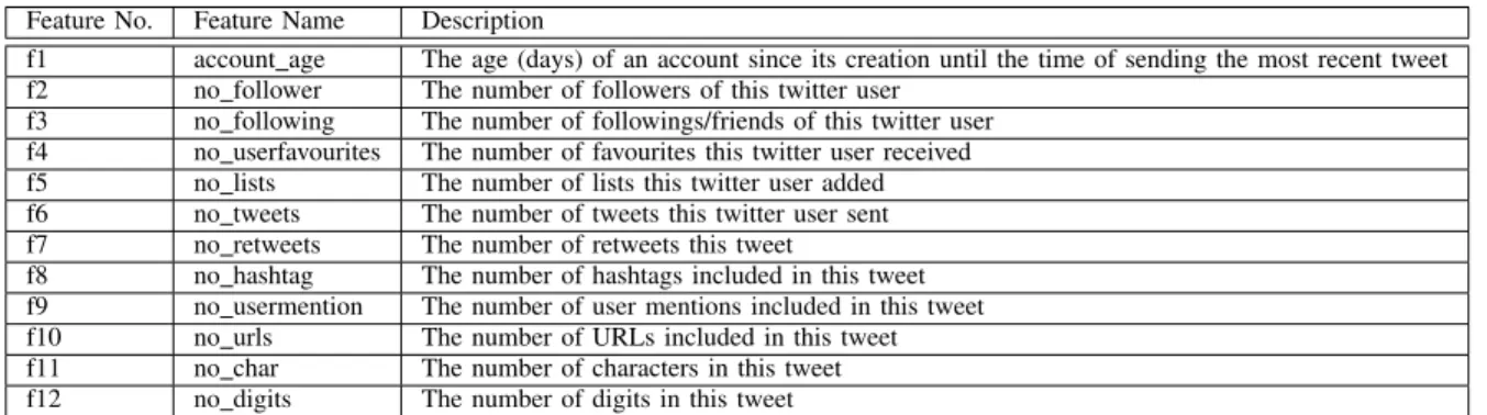
Feature No. Feature Name Description
f1 account age The age (days) of an account since its creation until the time of sending the most recent tweet f2 no follower The number of followers of this twitter user
f3 no following The number of followings/friends of this twitter user f4 no userfavourites The number of favourites this twitter user received f5 no lists The number of lists this twitter user added f6 no tweets The number of tweets this twitter user sent f7 no retweets The number of retweets this tweet
f8 no hashtag The number of hashtags included in this tweet f9 no usermention The number of user mentions included in this tweet f10 no urls The number of URLs included in this tweet f11 no char The number of characters in this tweet f12 no digits The number of digits in this tweet
We apply Trend Micro’s Web Reputation Technology to identify which tweets are deemed spam [4]. Trend Micro’s WRT system maintains a large dataset of URL reputation records, which are derived from their customers’ opt-in URL filtering records. WRT system is dedicated to collecting the latest and the most popular URLs, to analysing them, and then to providing Trend Micro customers with real-time protection while they are surfing the web. Hence, through checking URLs with the WRT system, we are able to identify whether a URL is malicious or not. We define those which contain malicious URLs as Twitter spam. In our collected data, we labelled one million spam tweets and one million non-spam tweets for 10 days, with 100k spam tweets and 100k non-spam tweets for each day.
Feature extraction is a key component in machine learning based classification tasks [37]. Some studies [1], [30], [33] have applied a few features which make use of historical in-formation of a user, such as tweets that the user sent in a period of time. While these features may be more discriminative, it is not possible to collect them due to the restrictions of Twitter’s API. Other researchers [29], [34] applied some social graph based features, which are hard to be evaded. Nevertheless, It is significantly expensive to collect those features, as they cannot be calculated until the social graph is formed. Thus, those expensive features are not suitable for real-time detection, despite that they have more discriminative power in separating spammers and legitimate users. The longer time a spam tweet exists, the more chance it can be exposure to victims. Thus, it is very important to detect spam tweets as early as possible. To reduce the loss caused by spam, real-time detection is in demand. Consequently, we only focus on extracting light-weight features which can be used for timely detection. These features can be straightforwardly extracted from the collected tweets’ JSON data structure [23] with little computation. We have totally extracted 12 features from our dataset as listed in TABLE I.
B. Problem Statement
In the real world, the statistical features of spam tweets are changing in unpredicted ways over time. As a result, machine learning based detection system becomes inaccurate. The issue is referred to as “Spam Drift” problem in our previous paper [5]. Here, we present an investigation of “Spam Drift” problem
from the aspect of the change of mean value of each feature from day to day.
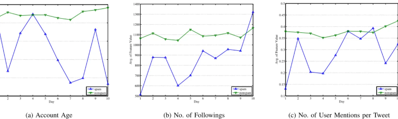
Fig. 1 shows the changing trend of average value of each feature for two classes in 10 days. In general, the variation of average value of feature from spam tweets is greater than that of non-spam tweets. Fig. 1a shows that, the average value of Account Age for spam tweets ranges from 530 to 730, and the variation is dramatic. However, it deviates from 710 to 740 for non-spam tweets, which is relatively stable. It is due to the fact that spammers are creating a large number of new accounts to send spam once their old account are blocked. For instance, we have 3 spammers with account age of 2 days, 6 days, 10 days in the first day, the average value of Account Age is (2 +6 +10) / 3 = 6 days. In the second day, if the spammer whose account age is 2 days is detected and removed, the average value of Account Age is (6+10) / 2 = 8 days, which increases. In addition, spammers may also generate new accounts with 0 day Account Age to spread spam after some of their accounts are block, which can lead the decrease of average value of Account Age. That is why the average value of Account Age is fluctuating. Naturally, spammers tend to keep following new friends as they want to be exposed to public more frequently, whereas for non-spammers, their number of followings are not changing too much once they have built their friend circle, as we can see from Fig. 1c. As expected, most of the other features have the same trend: the average value of one feature varies for spam tweets, while it is stable for non-spam tweets. To sum up, the characteristics of spam tweets is varying from day to day, while that of non-spam tweets is not changing much, as we see from Fig. 1. “Spam Drift” is a crucial issue in Twitter spam detection, which is in great need to be solved.
C. Problem Justification
In previous section, we simply compare some representative statistics, such as the mean values of features to show the “Spam Drift” problem. To further illustrate the changing of the statistical features in a dataset, a natural approach is to model the distribution of the data [8]. There are two kinds of approaches: parametric and non-parametric. Parametric approaches are very powerful when the specific distribution of the dataset, like Normal Distribution, is already known. However, the distribution of the Twitter spam data is unknown, thus it is not possible to apply parametric approaches. Con-sequently, non-parametric methods, such as statistical tests,
1 2 3 4 5 6 7 8 9 10 500 550 600 650 700 750 Day
Avg. of Feature Value
spam nonspam
(a) Account Age
1 2 3 4 5 6 7 8 9 10 500 600 700 800 900 1000 1100 1200 1300 1400 Day
Avg. of Feature Value
spam nonspam (b) No. of Followings 1 2 3 4 5 6 7 8 9 10 0.1 0.15 0.2 0.25 0.3 0.35 0.4 0.45 0.5 Day
Avg. of Feature Value
spam nonspam
(c) No. of User Mentions per Tweet
Fig. 1: Changes of Average Values of Features
TABLE II: KL Divergence of Spam and Nonspam Tweets of two Consecutive Days
D1 VS D2 D2 VS D3 D3 VS D4 D4 VS D5 D5 VS D6 D6 VS D7 D7 VS D8 D8 VS D9 D9 VS D10 f1 0.36 0.04 0.34 0.03 0.44 0.04 0.24 0.03 0.26 0.03 0.27 0.03 0.29 0.05 0.26 0.03 0.34 0.04 f2 0.24 0.1 0.22 0.1 .26 0.1 0.19 0.1 0.21 0.1 0.21 0.1 0.17 0.1 0.38 0.1 0.35 0.1 f3 0.28 0.07 0.22 0.07 0.32 0.07 0.15 0.07 0.22 0.07 0.2 0.07 0.2 0.08 0.26 0.08 0.23 0.08 f4 0.16 0.07 0.13 0.07 0.14 0.08 0.14 0.07 0.17 0.07 0.19 0.07 0.13 0.07 0.27 0.08 0.19 0.08 f5 0.02 0.01 0.02 0.01 0.03 0.01 0.02 0.01 0.01 0.01 0.02 0.01 0.01 0.01 0.05 0.01 0.05 0.01 f6 0.98 0.35 0.52 0.35 0.63 0.35 0.36 0.35 0.45 0.34 0.4 0.34 0.45 0.35 0.5 0.35 0.52 0.36 f7 0.1 0.04 0.08 0.03 0.04 0.04 0.04 0.04 0.05 0.03 0.07 0.04 0.06 0.04 0.1 0.04 0.08 0.04 f8 0.19 0 0 0 0.04 0 0.03 0 0.02 0 0.03 0 0.01 0 0.04 0 0.02 0 f9 0.09 0 0.03 0 0.01 0 0.02 0 0.01 0 0.01 0 0 0 0.04 0 0.01 0 f10 0 0 0.03 0 0.03 0 0.01 0 0.1 0 0 0 0.01 0 0.32 0 0.27 0 f11 0.26 0.01 0.06 0.01 0.06 0.01 0.11 0.01 0.1 0 0.09 0 0.26 0.01 0.28 0.01 0.2 0.02 f12 0.04 0 0 0 0.02 0 0.03 0.01 0.03 0 0.04 0 0.04 0 0.46 0 0.46 0 Original spam Changed spam Decision Boundary Non-spam
Fig. 2: Illustration of “Spam Drift”
which make no assumptions of the dataset distributions are used by researchers [11].
The statistical tests are to compute the distance of two distributions to determine the change. One of the most com-mon measures to compute the distance of distributions is Kullback-Leibler (KL) Divergence [8], [27]. The suitability of KL Divergence to be used in measuring distributions can be found in [8]. KL Divergence, which is also known as relative
entropy is defined as Dkl(PkQ) = X i P(i)logP(i) Q(i).
It is used to compare two probability distributions. We need to map data points into distributions to apply the formula. According to [7], lets={x1, x2, . . . , xn}be a multi-set from
a finite setFcontaining numerical feature values, and denote
N(x|s)the number of appearances ofx∈s, thus the relative proportion of each xis donated by
Ps(x) =
N(x|s) n .
However, the ratio of p/q is undefined if Q(i) = 0. As suggested by [18], the estimatePs is replaced as,
Ps(x) =
N(x|s) + 0.5 n+|F|/2 .
when |F| is number of elements in the finite set F. The distance between two day’s tweets, D1 andD2is,
D(D1kD2) =X x∈F PD1(x)log PD1(x) PD2(x) .
We compute the KL Divergence of each feature of spam and non-spam tweets in two adjacent days, which is listed in TABLE II. The shadowed ones are the KL Divergence of features of non-spam tweets, while the others are the KL Divergence of features of spam tweets. KL Divergence indicates the dissimilarity of two distributions. The larger the
5)&ODVVLILHU 6SDPWZHHWV LDT /DEHOOHGWZHHWV 8QODEHOOHGWZHHWV 1RQVSDPWZHHWV LHL 5)&ODVVLILHU
8QODEHOOHGWZHHWV 3UWę5 $FWLYHO\
ODEHOOHGWZHHWV
5)&ODVVLILHU
7HVWLQJWZHHWV &ODVVLILFDWLRQ5HVXOWV
Spam tweets
Fig. 3: Lfun Framework
value is, the more different the two distributions are. As shown in Table II, the KL Divergence of spam tweets in two adjacent days are much larger than that of the non-spam tweets for more than half the features. Taking f1 (”account age”) for example, the KL Divergence of spam between Day 1 and Day 2 is 0.36, while it is only 0.04 for non-spam, which indicates that the distribution of f1 of spam in Day 1 is much different to it in D2, compared with non-spam tweets’ distribution. From these KL Divergence values, we can see that the distribution of spam tweets’ features is changing unpredictably from day to day. Nevertheless, the distribution of training data is unchanged. As the knowledge structure which learns from the unchanged training data is not updated while being used to classify new incoming tweets, the performance of classifiers becomes inaccurate. As it is illustrated in Fig. 2, while the spam changes, the decision boundary is not updated. Consequently, more spam tweets are misclassified as non-spam.
IV. PROPOSEDSCHEME:Lfun
Existing machine learning based spam detection methods suffer from the problem of “Spam Drift” due to the change of statistical features of spam tweets as time goes on. When “spam drifts”, the old classification model is not updated with “changed” spam samples, as a result, the classification results will gradually become inaccurate. To solve this problem, obtaining the “changed” samples to update the classification model is very important. By observing that there are such samples in the unlabelled incoming tweets which are very easy to collect, we propose a scheme called “Lfun” to address “Spam Drift” problem.
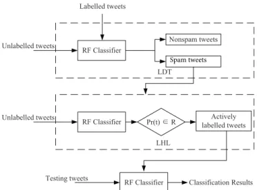
This section presents our Lfun scheme to deal with the drift problem in Twitter spam detection. Fig. 3 illustrates the framework of our proposed scheme. There are two main components in this framework: LDT is to learn from detected spam tweets and LHL is to learn from human labelling. In “Drifted Spam Detection” scenario, we have already got a small amount of labelled spam and non-spam tweets. How-ever, there are not enough samples of “changed” spam. It is
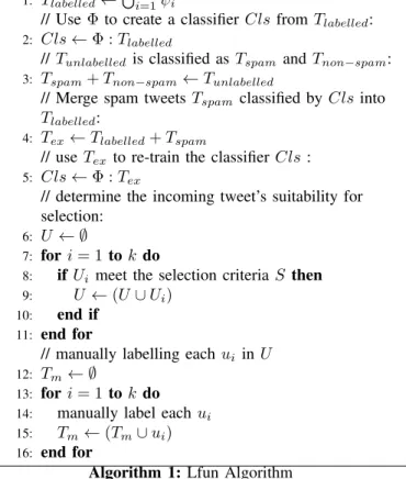
extraordinary expensive to have human label a large amount of “changed” tweets. Consequently, we make use of the above mentioned two components to automatically extract “changed” spam tweets from a set of unlabelled tweets, which are very easy to collected from Twitter. Once getting enough labelled “changed” spam tweets, we implement the scheme which employs a sufficiently powerful algorithm, Random Forest, to perform classification. Our Lfun scheme is summarised in Algorithm 1.
A. Learning from Detected Spam Tweets
LDT is used to deal with a classification scenario where there is a sufficiently robust algorithm, but in lack of more data [25]. By learning from a large number of unlabelled data, LDT can obtain sufficient new information, which can be used to update the classification model.
In a LDT learning scenario, we are given a labelled data set Tl = {(x1, y1),(x2, y2), . . . ,(xm, ym)}, containing m
labelled tweets, where xi ∈ Rk(i = 1,2, . . . , m) is the
feature vector of a tweet, yi ∈ {spam, non−spam} is the
category label of a tweet. We are also given a large data set Tu ={xm+1, ym+1),(xm+2, ym+2), . . . ,(xm+n, ym+n)}
containingnunlabelled tweets (n >> m). Then a classifierϕ
is trained byTl.ϕcan be used to divideTu into spamTspam
and non-spamTnon−spam. Labelled spam tweets fromTuwill
be added into the labelled data setTl to form a new training
data set.
The basic of LDT is to find a function ϕ : Rk −→
{spam, non−spam}to predict the labely∈ {spam, non−
spam}of new tweets when trained byTl+spam, which is the
combination of the labelled data setTland spam tweetsTspam
identified fromTu. Particularly, the unlabelled data setTuused
in LDT does not have to share the same distribution with the labelled data setTl[16]. In addition, only detected spam tweets
will be added into the training data. The reason is that, we’ve already gained sufficient information of non-spam tweets, as the statistical properties are not changing for non-spam tweets. It is not necessary for us to gain more information about non-spam tweets.
However, the spam tweets detected by the classifier that is trained using Tl also have the same or similar distribution of
old spam. We need samples from “changed spam” to calibrate the classifier. We then use LHL (in Section IV-B) to get “changed spam” samples.
B. Learning from Human Labelling
In a supervised spam detection system, a learning algorithm, such as Random Forest, must be trained by sufficient labelled data to obtain more accurate detection results. However, la-belled instances are very expensive and time-consuming to obtain. Fortunately, we have a huge number of unlabelled tweets which can be easily collected. The LHL in our Lfun is best suited where there are numerous unlabelled data instances, and human annotator anticipating to label many of them to train an accurate system [28]. LHL aims to minimize the labelling cost by using different learning criteria to select most informative samples from unlabelled data to be labelled by a
Require: labelled training set{ψ1, ..., ψN},
unlabelled tweetsTunlabelled,
a binary classification algorithmΦ,
Ensure: manually labelled selected tweetsTm
1: Tlabelled←S N i=1ψi
// UseΦto create a classifierClsfromTlabelled:
2: Cls←Φ :Tlabelled
//Tunlabelled is classified asTspam andTnon−spam:
3: Tspam+Tnon−spam←Tunlabelled
// Merge spam tweetsTspam classified byClsinto
Tlabelled:
4: Tex←Tlabelled+Tspam
// useTex to re-train the classifierCls:
5: Cls←Φ :Tex
// determine the incoming tweet’s suitability for selection:
6: U ← ∅
7: fori= 1 tok do
8: ifUi meet the selection criteriaS then
9: U ←(U∪Ui)
10: end if 11: end for
// manually labelling eachui inU
12: Tm← ∅
13: fori= 1 tok do 14: manually label eachui
15: Tm←(Tm∪ui)
16: end for
Algorithm 1: Lfun Algorithm
human annotator [39]. We also import active learning in our Lfun scheme.
Now let us define our learning component in a for-mal way. In supervised Twitter spam detection, we are given a labelled training data set Ttraining =
{(x1, y1),(x2, y2), . . . ,(xm, ym)}, containing m labelled
tweets, wherexi∈Rk(i= 1,2, . . . , m)is the feature vector of
a tweet,yi∈ {spam, non−spam}is the category label of a
tweet. The labelyi of a tweetxiis donated asy=f(x). The
task is then to learn a functionfˆwhich can correctly classify a tweet to spam or non-spam. We use generalisation error to measure the accuracy of the learned function:
Error( ˆf) = X
x∈Ttraining
Lf(x),f(ˆx)P(x).
In practice, f(x) is not available for testing data instances. Therefore, it is usual to estimate the generalisation error by the test error:
Error( ˆf) = X
x∈Ttesting
Lf(x),f(ˆx)P(x),
whereTtestingrefers to the testing tweets, and prediction error
can be measured by a loss function L, such as mean squared error (MSE) [26]: LM SE f(x),f(ˆx)=f(x)−f(ˆx) 2 .
The learning criteria is set to select the most useful instances
Xselectedand add them to the training setTtrainingfor
achiev-ing some certain objectives. Let us consider this objective as the minimization of generation error of a learned function trained by Ttraining. So the learning criteria can be donated
as
Error(Ttraining∪ {Xselected}).
The goal of this kind of learning is to select instances
Xselected which can minimize the generalisation error
Error(Xselected):
argmin Error(Xselected).
As a result, good selection criteria must be estimated to minimize the error. In Lfun scheme, we apply the selection criteria, called “Probability Threshold Filter Model”, to select the most informative tweets to tackle “Spam Drift”. In order to achieve this, Random Forest (RF) is used to determine the probability of a tweet whether it belongs to spam or not. Random Forest [2] can generate many classification trees after being trained withTexfrom Asymmetric Self-Learning. When
classifying a new incoming tweet, each tree in the forest will give a class prediction. Then forest chooses the classification result which has the most votes. In our case, we set the number of trees tom, ifntrees vote for the class “spam”, the probability of the tweet to be classified as “spam” isP r=mn. Through our empirical study, the mis-classification mostly occurred when P r ∈[0.4,0.7]. So we set the threshold τ to
P r ∈[0.4,0.7]. After we pre-filter some candidate tweets to be labelled using the “Probability Threshold Filter Model”, the number of tweets is still too many. We then randomly select a smaller number of tweets from the candidate tweets (we set it to be 100 in our experiments) to be manually labelled. As shown in Fig. 3, the manually labelled tweets, along withTex
will be used to train a new classifier, which can tackle “Spam Drift” problem.
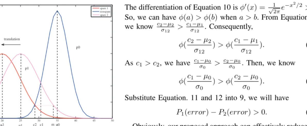
C. Performance Benefit Justification
We study the performance benefit of the proposed Lfun scheme by providing the theoretical analysis in this section. Fig. 4 illustrates the performance benefit by using simulation. We use three normal distributions (listed below) to simulate this:w0represents the distribution of non-spam, whilew1and
w2 represents the distribution of spam before and after using
our Lfun approach, respectively. w0∼N(µ0, σ20) w1∼N(µ1, σ212) w2∼N(µ2, σ212)
The PDFs (probability distribution functions) [9] of these three distributions, w0, w1 and w2 are illustrated as p0, p1
and p2 in Fig. 4. We assume that only the mean µ1 of w1
changes toµ2, but the varianceσ12 is not changing.
As p1 translated to p2, we can always find m, which can
make
0 5 10 15 20 25 30 35 40 45 50 0 0.02 0.04 0.06 0.08 0.1 0.12 0.14 spam 1 nonspam spam 2 p0 p2 p1 translation u2 u1 c2 c1 m u0
Fig. 4: Performance Benefit Illustration
and p1(m) =p2(c2). (2) Asc2< c1, we have p0(c2)< p0(c1). (3) We also have p0(c1) =p1(c1), p0(c2) =p2(c2). (4)
From Equation. 3 and Equation. 4, we get
p1(c1)> p2(c2). (5)
From Equation. 2 and Equation. 5, we can have
p1(c1)> p1(m). (6)
As a result,
m > c1. (7)
Taking into account Equation. 7 and Equation. 1, we can have
c1−c2< µ1−µ2. So,
c2−µ2> c1−µ1. (8)
The error rate of classification before Lfun,
P1(error) =P(x > c1) +P(x < c2) = Z ∞ c1 p1(t)dt+ Z c1 −∞ p0(t)dt = 1−φ(c1−µ1 σ12 ) +φ(c1−µ0 σ0 ).
Similarly, we have the error rate after using Lfun
P2(error) = 1−φ( c2−µ2 σ12 ) +φ(c2−µ0 σ0 ).
The difference of P1(error)andP2(error),
P1(error)−P2(error) =hφ(c2−µ2 σ12 )−φ( c1−µ1 σ12 ) i +hφ(c1−µ0 σ0 )−φ( c2−µ0 σ0 ) i , (9) while φ(x) = √1 2π Z x 0 e−t2/2dt. (10)
The differentiation of Equation 10 isφ0(x) = √1
2πe
−x2/2
>0. So, we can haveφ(a)> φ(b)when a > b. From Equation. 8, we know c2−µ2 σ12 > c1−µ1 σ12 . Consequently, φ(c2−µ2 σ12 )> φ(c1−µ1 σ12 ). (11)
Asc1> c2, we have c1σ−0µ0 > c2σ−0µ0.Then, we know
φ(c1−µ0 σ0
)> φ(c2−µ0 σ0
). (12)
Substitute Equation. 11 and 12 into 9, we will have
P1(error)−P2(error)>0. (13)
Obviously, our proposed approach can effectively reduce the probability of error from Equation 13.
V. PERFORMANCEEVALUATION
In this section, we evaluate the performance of the proposed Lfun scheme in detecting “drifted” Twitter spam. All the experiments are carried out on our real-world 10 consecutive days’ tweets with each day containing 100k spam tweets and 100k non-spam tweets.
As in existing works [34], we also use F-measure and
Detection Rateto measure the performance. Despite that both
of the metrics are used to evaluate all the classes’ performance, we only focus on the F-measure and Detection Rate of spam class. F-measure is an evaluation metric which combines precision and recall to measure the per-class performance of classification or detection algorithms. It can be calculated by
F−measure= 2∗P recision∗Recall P recision+Recall .
Detection Rate is defined as the ratio of those tweets correctly classified as belonging to classspam to the total number of tweets in class spam, it can be calculated by
DetectionRate= T P T P+F N.
In the evaluation, we have designed three sets of experi-ments in order to show the impact of spam drift (in Section V-A) firstly, then the benefit of our proposed Lfun (in Section V-B) and the comparisons with other traditional machine learn-ing algorithms (in Section V-C). We repeat the experiments for 100 times with different random training samples and report the average values on all the 100 runs.
A. Impact of Spam Drift
In order to evaluate the impact of “Spam Drift” problem, we perform a number of experiments in this section. It is aiming to show that the performance of a traditional classifier, for example C4.5 Decision Tree, varies over time when “Spam Drift” exists.
During these experiments, Day 1 data is divided into two parts, half for training pool where training data can be ex-tracted from, and another half for testing purpose. We create a classifier by using a supervised classification algorithm, and train it with 10k spam and 10k non-spam tweets which are randomly sampled from the training pool of Day 1. Then the
1 2 3 4 5 6 7 8 9 10 0 0.1 0.2 0.3 0.4 0.5 0.6 0.7 0.8 0.9 1 Day Detection Rate spam nonspam
(a) Random Forest
1 2 3 4 5 6 7 8 9 10 0 0.1 0.2 0.3 0.4 0.5 0.6 0.7 0.8 0.9 1 Day Detection Rate spam nonspam (b) C4.5 Decision Tree 1 2 3 4 5 6 7 8 9 10 0 0.1 0.2 0.3 0.4 0.5 0.6 0.7 0.8 0.9 1 Day Detection Rate spam nonspam (c) Bayes Network
Fig. 5: Trend of Detection Rate
classifier is used to classify the testing data in Day1, as well as the testing samples in Day 2 to Day 10.
Fig. 5 shows the Detection Rate of both spam and non-spam tweets on three classifiers, Random Forest, C4.5 Decision Tree and Bayes Network. We can see that, the Detection Rate of non-spam is very stable, it keeps above 90% for Random Forest and C4.5 Decision Tree, and near 90% for Bayes Network, despite the change of testing data. However, when it comes to spam tweets, the Detection Rate fluctuates dramatically, and the overall trend is decreasing. The Detection Rates for Random Forest and C4.5 Decision Tree are 90% in the first day, but they could decrease to less then 40% in the 9th day. This phenomenon also applies with Bayes Network, the Detection Rate decreases from 70% on 1st day to less than 50% for most of the other testing days.
B. Performance of Lfun
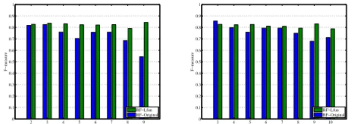
We evaluate the performance of Lfun here, by using F-measure and Detection Rate. The number labelled training samples from old day (i.e.Day 1 and Day 2 in this case) is 5000. The number of manually labelled samples during Lfun is set to 100.
Fig. 6 shows the Detection Rate of Lfun, when Day 1 data (Fig. 6a) or Day 2 data (Fig. 6b) is used for training and the rest days are used for testing. We can see from Fig. 6a that, the Detection Rates of original Random Forest are relatively low. For example, the Detection Rate when testing on Day 9 is only around 40%. However, our RF-Lfun can reach over 90% Detection Rate on the same day. While Random Forest can only achieve Detection Rate ranging from 45% to 80%, our RF-Lfun can rise as high as 90% Detection Rate. This also happens when training data is from Day 2, and testing data is from Day 3 to Day 10, as illustrated in Fig. 6b. The highest Detection Rate of Random Forest is around 85%, but that of RF-Lfun is over 95%. Generally, our Lfun can detect most of the spam tweets even with “Spam Drift”. The reason is that, our Lfun brings more samples of “changed spam tweets” to update the training process.
Fig. 7 shows the F-measure of Random Forest using Lfun approach compared with it without using Lfun. We can see that, the F-measure of original Random Forest keeps
decreas-2 3 4 5 6 7 8 9 0 0.1 0.2 0.3 0.4 0.5 0.6 0.7 0.8 0.9 1 Day Detection Rate RF−Lfun RF−Original
(a) Day 1 training, Day 2 to 9 testing
3 4 5 6 7 8 9 10 0 0.1 0.2 0.3 0.4 0.5 0.6 0.7 0.8 0.9 1 Day Detection Rate RF−Lfun RF−Original
(b) Day 2 training, Day 3 to 10 testing
Fig. 6: Detection Rate of Lfun
2 3 4 5 6 7 8 9 0 0.1 0.2 0.3 0.4 0.5 0.6 0.7 0.8 0.9 1 Day F−measure RF−Lfun RF−Original
(a) Day 1 training, Day 2 to 9 testing
3 4 5 6 7 8 9 10 0 0.1 0.2 0.3 0.4 0.5 0.6 0.7 0.8 0.9 1 Day F−measure RF−Lfun RF−Original
(b) Day 2 training, Day 3 to 10 testing
Fig. 7: F-measure of Lfun
ing from 80% to 55% as the testing data changes from Day 2 to Day 9 in Fig. 7a. However, once it is applied with our Lfun approach, the F-measure becomes stable, which is always greater than 80%, except on Day 8. Similarly, when the training data is from Day 2, F-measure of Random Forest is decreasing as well. But F-measure of our Lfun-RF is not fluctuating, as shown in Fig. 7b. Nevertheless, the proposed Lfun can effectively improve the F-measure and the improvement is up to 25% in the best case.
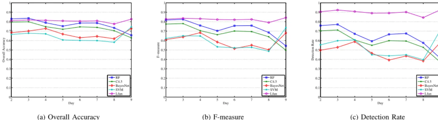
C. Comparisons with other Algorithms
In this section, we compare our Lfun approach with four traditional machine learning algorithms (Random Forest, C4.5
Decision Tree, Bayes Network and SVM) to detect spam tweets
in the “drift” scenario. There are two sets of experiments carried out. One set is to evaluate the performance while
training data is from Day 1, and testing data are varying from Day 2 to Day 9. Another set is to evaluate the performance when training and testing data are from two specified days, but the number of labelled training data is changing from 1000 to 10000.
1) Comparisons with Changing Days: Fig. 8 demonstrates
the experimental results in terms of overall accuracy, F-measure and detection rate of Lfun compared to other algo-rithms, when the testing days are varying. We can see from Fig. 8a that, the overall accuracy of Lfun outperforms all the other algorithms, followed by Random Forest, C4.5 Decision Tree, Bayes Network and SVM. In terms of F-measure (see Fig. 8b), our Lfun is also the best among all the algorithms. For example, it is over 30% higher than C4.5 Decision Tree when testing data is from Day 9. Furthermore, the performance of Lfun is much better in terms of detection rate. Fig. 8c show that, the detection rate of Lfun is above 90% for most of the days. However, the detection rate of all the others is below 80%. Especially, Bayes Network has the lowest detection rate, which is below 50%. In general, our Lfun is the best among all the algorithms evaluated by all the three metrics.
2) Comparisons with Changing Labelled Training Samples:
Fig. 9 and Fig. 10 report the evaluation results when the number of labelled training samples is changing. The training and testing data is from Day 1 and Day 5 in Fig. 9, while the training and testing data is from Day 4 and Day 8 in Fig. 10. We can see that the overall accuracy of Lfun increases from 70% to 80% with the increase of labelled training samples. It is better than the four algorithms in comparison, as the best of them (C4.5 Decision Tree) can only achieve less than 74% overall accuracy. When it comes to F-measure, the performance of Lfun is still the best; it is 10% higher than that of C4.5 Decision Tree and nearly 30% higher than that of SVM. In terms of detection rate, our Lfun is about 30% higher than the second best algorithm. Similarly in Fig. 10, Lfun outperforms all the other algorithms.
VI. DISCUSSIONS
In research community, there are also some machine learn-ing approaches related to our proposed method. For exam-ple, online learning and incremental learning. They are both common machine learning algorithms to continuously update the prediction model with new training data for better future classification. They can generate a prediction model and put it into operation without much training data at first, but they require new training data to update the model. When it comes to online Twitter spam classification, it is very difficult to label enough training samples to update the model. The reasons are two-folds. Firstly, it is significantly time-consuming to label a large amount of tweets by human. Secondly, it is difficult to gain enough spam tweets even we have got a large number of human-labelled tweets, as the spam rate of Twitter is about 5% [6]. If there are not enough spam samples (Lfun does not need non-spam samples as non-spam tweets are not drifting) to retrain the model, it is not able to solve the “spam drift” issue.
Our Lfun approach has the same advantage of online learning and incremental learning, i.e., it can be deployed
without much training data at the beginning, but to be up-dated when new training data comes. Different to online and incremental learning, we incorporate both automated labelling and human labelling. The LDT component learns from the detected tweets. This competent is automatically updated with detected spam tweets with no human effort. To better adjust the prediction model, we also import LHL component, which learns from human labelling. To minimize human effort, LHL only samples a very small number of tweets for labelling, for example, 100 tweets in our experiments. In addition, it does not randomly pick up tweets to label, but to be in line with selection criteria called “Probability Threshold Filter Model” which can choose the most useful tweets. Benefiting from these two components, our Lfun approach can successfully deal with “spam drift”, but with the least human effort.
VII. CONCLUSION ANDFUTUREWORK
In this paper, we firstly identify the “Spam Drift” problem in statistical features based Twitter spam detection. In order to solve this problem, we propose a Lfun approach. In our Lfun scheme, classifiers will be re-trained by the added “changed spam” tweets which are learnt from unlabelled samples, thus it can reduce the impact of “Spam Drift” significantly. We evaluate the performance of Lfun approach in terms of De-tection Rate and F-measure. Experimental results show that both detection rate and F-measure are improved a lot when applying with our Lfun approach. We also compare Lfun to four traditional machine learning algorithms, and find that our Lfun outperforms all four algorithms in terms of overall accuracy, F-measure and Detection Rate.
There is also a limitation in our Lfun scheme. The benefit of “old” labelled spam is to eliminate the impact of “spam drift” to classify more accurate spam tweets in future days. The effectiveness of “old” spam has been proved by our experiments during a short period. However, the effectiveness will decrease as the correlation of “very old” spam becomes less with the new spam in the long term run. In the future, we will incorporate incremental adjustment to adjust the training data, such as dropping the “too old” samples after a certain time. It can not only eliminate unuseful information in the training data but also make it faster to train the model as the number of training samples decrease.
ACKNOWLEDGMENT
The authors would like to thank Trend Micro for providing us the service to label spam tweets. This work is supported by ARC Linkage Project LP120200266.
REFERENCES
[1] F. Benevenuto, G. Magno, T. Rodrigues, and V. Almeida. Detecting spammer on twitter. In Seventh Annual Collaboration, Electronic messaging, Anti-Abuse and Spam Conference, July 2010.
[2] L. Breiman. Random forests. Machine Learning, 45(1):5–32, 2001. [3] C. Castillo, M. Mendoza, and B. Poblete. Information credibility on
twitter. InProceedings of the 20th international conference on World wide web, WWW ’11, pages 675–684, New York, NY, USA, 2011. ACM.
2 3 4 5 6 7 8 9 0 0.1 0.2 0.3 0.4 0.5 0.6 0.7 0.8 0.9 1 Day Overall Accuracy RF C4.5 BayesNet SVM Lfun
(a) Overall Accuracy
2 3 4 5 6 7 8 9 0 0.1 0.2 0.3 0.4 0.5 0.6 0.7 0.8 0.9 1 Day F−measure RF C4.5 BayesNet SVM Lfun (b) F-measure 2 3 4 5 6 7 8 9 0 0.1 0.2 0.3 0.4 0.5 0.6 0.7 0.8 0.9 1 Day Detection Rate RF C4.5 BayesNet SVM Lfun (c) Detection Rate
Fig. 8: Comparisons with other Algorithms (changing testing days)
10000 2000 3000 4000 5000 6000 7000 8000 9000 10000 0.1 0.2 0.3 0.4 0.5 0.6 0.7 0.8 0.9 1
No. of Labelled Traning Samples
Overall Accuracy RF C4.5 BayesNet SVM Lfun
(a) Overall Accuracy
10000 2000 3000 4000 5000 6000 7000 8000 9000 10000 0.1 0.2 0.3 0.4 0.5 0.6 0.7 0.8 0.9 1
No. of Labelled Traning Samples
F−measure RF C4.5 BayesNet SVM Lfun (b) F-measure 10000 2000 3000 4000 5000 6000 7000 8000 9000 10000 0.1 0.2 0.3 0.4 0.5 0.6 0.7 0.8 0.9 1
No. of Labelled Traning Samples
Detection Rate RF C4.5 BayesNet SVM Lfun (c) Detection Rate
Fig. 9: Comparisons with other Algorithms (training on Day 1 and testing on Day 5)
10000 2000 3000 4000 5000 6000 7000 8000 9000 10000 0.1 0.2 0.3 0.4 0.5 0.6 0.7 0.8 0.9 1
No. of Labelled Traning Samples
Overall Accuracy RF C4.5 BayesNet SVM Lfun
(a) Overall Accuracy
10000 2000 3000 4000 5000 6000 7000 8000 9000 10000 0.1 0.2 0.3 0.4 0.5 0.6 0.7 0.8 0.9 1
No. of Labelled Traning Samples
F−measure RF C4.5 BayesNet SVM Lfun (b) F-measure 10000 2000 3000 4000 5000 6000 7000 8000 9000 10000 0.1 0.2 0.3 0.4 0.5 0.6 0.7 0.8 0.9 1
No. of Labelled Traning Samples
Detection Rate RF C4.5 BayesNet SVM Lfun (c) Detection Rate
Fig. 10: Comparisons with other Algorithms (training on Day 4 and testing on Day 8)
[4] C. Chen, J. Zhang, X. Chen, Y. Xiang, and W. Zhou. 6 million spam tweets: A large ground truth for timely twitter spam detection. In
IEEE ICC 2015 - Communication and Information Systems Security Symposium (ICC’15 (11) CISS), pages 8689–8694, London, United Kingdom, June 2015.
[5] C. Chen, J. Zhang, Y. Xiang, and W. Zhou. Asymmetric Self-Learning for tackling twitter spam drift. InThe Third International Workshop on Security and Privacy in Big Data (BigSecurity 2015), pages 237–242, Hong Kong, Hong Kong, Apr. 2015.
[6] C. Chen, J. Zhang, Y. Xiang, W. Zhou, and J. Oliver. Spammers are becoming smarter on twitter.IT Professional, 18(2):14–18, Mar.-April. 2016.
[7] I. Csiszar and J. K¨orner. Information theory: coding theorems for discrete memoryless systems. Cambridge University Press, 2011. [8] T. Dasu, S. Krishnan, S. Venkatasubramanian, and K. Yi. An
information-theoretic approach to detecting changes in multi-dimensional data streams. In In Proc. Symp. on the Interface of Statistics, Computing Science, and Applications, 2006.
[9] R. O. Duda, P. E. Hart, and D. G. Stork. Pattern Classification (2Nd Edition). Wiley-Interscience, 2000.
[10] M. Egele, G. Stringhini, C. Kruegel, and G. Vigna. Compa: Detecting compromised accounts on social networks. In Annual Network and Distributed System Security Symposium, 2013.
[11] J. a. Gama, I. ˇZliobait˙e, A. Bifet, M. Pechenizkiy, and A. Bouchachia. A survey on concept drift adaptation.ACM Comput. Surv., 46(4):44:1– 44:37, Mar. 2014.
[12] H. Gao, Y. Chen, K. Lee, D. Palsetia, and A. Choudhary. Towards online spam filtering in social networks. InNDSS, 2012.
[13] H. Gao, J. Hu, C. Wilson, Z. Li, Y. Chen, and B. Y. Zhao. Detecting and characterizing social spam campaigns. InProceedings of the 10th
ACM SIGCOMM conference on Internet measurement, IMC ’10, pages 35–47, New York, NY, USA, 2010. ACM.
[14] A. Greig. Twitter overtakes facebook as the most popular social network for teens, according to study.DailyMail, October 2013.
[15] C. Grier, K. Thomas, V. Paxson, and M. Zhang. @spam: the under-ground on 140 characters or less. InProceedings of the 17th ACM conference on Computer and communications security, CCS ’10, pages 27–37, New York, NY, USA, 2010. ACM.
[16] K. Huang, Z. Xu, I. King, M. Lyu, and C. Campbell. Supervised self-taught learning: Actively transferring knowledge from unlabeled data. InNeural Networks, 2009. IJCNN 2009. International Joint Conference on, pages 1272–1277, June 2009.
[17] R. Jeyaraman. Fighting spam with botmaker.Twitter Engineering Blog, August 2014.
[18] R. Krichevsky and V. Trofimov. The performance of universal encoding.
Information Theory, IEEE Transactions on, 27(2):199–207, Mar 1981. [19] H. Kwak, C. Lee, H. Park, and S. Moon. What is twitter, a social
network or a news media? InProceedings of the 19th international conference on World wide web, WWW ’10, pages 591–600, New York, NY, USA, 2010. ACM.
[20] K. Lee, J. Caverlee, and S. Webb. Uncovering social spammers: social honeypots + machine learning. InProceedings of the 33rd international ACM SIGIR conference on Research and development in information retrieval, SIGIR ’10, pages 435–442, New York, NY, USA, 2010. ACM. [21] S. Lee and J. Kim. Warningbird: A near real-time detection system for suspicious urls in twitter stream.IEEE Transactions on Dependable and Secure Computing, 10(3):183–195, 2013.
[22] J. Oliver, P. Pajares, C. Ke, C. Chen, and Y. Xiang. An in-depth analysis of abuse on twitter. Technical report, Trend Micro, 225 E. John Carpenter Freeway, Suite 1500 Irving, Texas 75062 U.S.A., September 2014.
[23] I. Ounis, C. Macdonald, J. Lin, and I. Soboroff. Overview of the trec-2011 microblog track. InProceeddings of the 20th Text REtrieval Conference (TREC 2011), 2011.
[24] C. Pash. The lure of naked hollywood star photos sent the internet into meltdown in new zealand. Business Insider, September 2014. [25] R. Raina, A. Battle, H. Lee, B. Packer, and A. Y. Ng. Self-taught
learning: transfer learning from unlabeled data. InProceedings of the 24th international conference on Machine learning, pages 759–766. ACM, 2007.
[26] N. Rubens, D. Kaplan, and M. Sugiyama. Active learning in recom-mender systems. InRecommender Systems Handbook, pages 735–767. Springer, 2011.
[27] R. Sebasti˜ao and J. a. Gama. Change detection in learning histograms from data streams. InProceedings of the Aritficial Intelligence 13th Portuguese Conference on Progress in Artificial Intelligence, EPIA’07, pages 112–123, Berlin, Heidelberg, 2007. Springer-Verlag.
[28] B. Settles. Active learning literature survey. University of Wisconsin, Madison, 52(55-66):11, 2010.
[29] J. Song, S. Lee, and J. Kim. Spam filtering in twitter using sender-receiver relationship. InProceedings of the 14th international conference on Recent Advances in Intrusion Detection, RAID’11, pages 301–317, Berlin, Heidelberg, 2011. Springer-Verlag.
[30] G. Stringhini, C. Kruegel, and G. Vigna. Detecting spammers on social networks. InProceedings of the 26th Annual Computer Security Applications Conference, ACSAC ’10, pages 1–9, New York, NY, USA, 2010. ACM.
[31] K. Thomas, C. Grier, J. Ma, V. Paxson, and D. Song. Design and evaluation of a real-time url spam filtering service. InProceedings of the 2011 IEEE Symposium on Security and Privacy, SP ’11, pages 447– 462, Washington, DC, USA, 2011. IEEE Computer Society.
[32] K. Thomas, C. Grier, D. Song, and V. Paxson. Suspended accounts in retrospect: an analysis of twitter spam. InProceedings of the 2011 ACM SIGCOMM conference on Internet measurement conference, IMC ’11, pages 243–258, New York, NY, USA, 2011. ACM.
[33] A. H. Wang. Don’t follow me: Spam detection in twitter. InSecurity and Cryptography (SECRYPT), Proceedings of the 2010 International Conference on, pages 1–10, 2010.
[34] C. Yang, R. Harkreader, and G. Gu. Empirical evaluation and new design for fighting evolving twitter spammers. Information Forensics and Security, IEEE Transactions on, 8(8):1280–1293, 2013.
[35] C. Yang, R. Harkreader, J. Zhang, S. Shin, and G. Gu. Analyzing spammers’ social networks for fun and profit: a case study of cyber criminal ecosystem on twitter. InProceedings of the 21st international conference on World Wide Web, WWW ’12, pages 71–80, New York, NY, USA, 2012. ACM.
[36] S. Yardi, D. Romero, G. Schoenebeck, and D. Boyd. Detecting spam in a twitter network. First Monday, 15(1-4), January 2010.
[37] J. Zhang, C. Chen, Y. Xiang, W. Zhou, and Y. Xiang. Internet traffic classification by aggregating correlated naive bayes predictions.
Information Forensics and Security, IEEE Transactions on, 8(1):5–15, Jan 2013.
[38] X. Zhang, S. Zhu, and W. Liang. Detecting spam and promoting campaigns in the twitter social network. InData Mining (ICDM), 2012 IEEE 12th International Conference on, pages 1194–1199, 2012. [39] I. Zliobaite, A. Bifet, B. Pfahringer, and G. Holmes. Active learning
with drifting streaming data.IEEE transactions on neural networks and learning systems, 25(1):27–39, 2014.