Experimental Approach Based on Ensemble and
Frequent Itemset Mining for Image Spam Filtering
Nor Azman Mat Ariff, Azizi Abdullah, Mohammad Faidzul Nasrudin
Center for Artificial Intelligence Technology,Faculty of Technology and Information Science, Universiti Kebangsaan Malaysia, 43600, Bangi,
Selangor Darul Ehsan, Malaysia. [email protected]
Abstract—Excessive amounts of image spam cause many
problems to e-mail users. Since image spam is difficult to detect using conventional text-based spam approach, various image processing techniques have been proposed. In this paper, we present an ensemble method using frequent itemset mining (FIM) for filtering image spam. Despite the fact that FIM techniques are well established in data mining, it is not commonly used in the ensemble method. In order to obtain a good filtering performance, a SIFT descriptor is used since it is widely known as effective image descriptors. K-mean clustering is applied to the SIFT keypoints which produce a visual codebook. The bag-of-word (BOW) feature vectors for each image is generated using a hard bag-of-features (HBOF) approach. FIM descriptors are obtained from the frequent itemsets of the BOW feature vectors. We combine BOW, FIM with another three different feature selections, namely Information Gain (IG), Symmetrical Uncertainty (SU) and Chi Square (CS) with a Spatial Pyramid in an ensemble method. We have performed experiments on Dredze and SpamArchive datasets. The results show that our ensemble that uses the frequent itemsets mining has significantly outperform the traditional BOW and naive approach that combines all descriptors directly in a very large single input vector.
Index Terms— Ensemble Methods; Frequent Itemset Mining;
Image Spam; SVM.
I. INTRODUCTION
E-mail was one of the earliest Internet services and still the most widely used today. It offers an efficient way to convey messages to the intended recipients and is often used in formal and informal communication. However, e-mail services also provide opportunities for marketers to promote their products in bulk using free bandwidth and storage. It is worsen when the malicious codes, such as malwares and viruses are also embedded [1]. This kind of e-mail is known as spam, it contains information that is unsolicited, inappropriate, and irrelevant [2].
At first, the spam e-mails are text-based and manipulate various text spam tricks including text splitting, encoding abuses, attack on tokenizer and symbolic text. In response, many effective text-based anti-spam filters were proposed, resulting in difficulties for the spam e-mails to pass through these filters. Spammers made attempts to outsmart the text-based filtering by embedding texts into images. An Optical Character Recognition (OCR) and content-based filtering are the two main approaches used by researchers in filtering image spam. The OCR approach is used by [3],[4],[5], extracting texts from images and analysing them, which is
similar to text processing. However, most of the approaches use content-based filtering because an OCR is an expensive process while spammers begin to introduce a variety of obscuring techniques, which make the OCR technique ineffective.
As the content-based filtering use the image processing techniques, several image features such as colour, edge and texture are usually exploited by the image spam filters [6]. A number of studies have demonstrated that colour features are among the most important factors and provide compact representation of images [3],[7],[8]. Even though the Scale Invariant Feature Transform (SIFT) as proposed by [9] is the most widely used image descriptor, there are very few studies [10] that investigated its impact on image spam filtering.
Most of the image spam researchers have performed global feature extraction where a global histogram is used to represent an image. One of the drawbacks with the global histogram is, it does not take spatial information into account which can provide high discrimination power. On the other hand, an image partitioning scheme such as the region-based approach and multi-resolution approach are more popular to be used in other image processing domains including the object recognition and scene category recognition [11],[12]. For example, if the spatial pyramid is applied to the images, each image has a number of representations from different levels of resolutions. The final implementation of the spatial pyramid is to perform a naïve approach by concatenating all feature vectors into one large input. However, instead of the naïve solution, we believe that full potential of image descriptors can be obtained if the ensemble method is applied to fuse multiple classifiers from each resolution level. The ensemble method works by combining classifiers in order to obtain one strong classifier which can outperform every one of them [13].
Bag-of-visual-words (BOW) is the most commonly used image representation among image classification methods. BOW can be extracted globally or locally from an image. In data mining community, frequent itemset mining techniques (FIM) are well established. FIM aims at finding sets of features that frequently exists together, which in many cases, can capture more discriminative information [14]. For example, in order to generate FIM descriptors from BOW, a frequent itemset of BOW can be generated by identifying a set of features that frequently exists together in the BOW feature vectors. However, it is unclear whether the classifiers generated from the FIM descriptors offer a good input as to the ensemble methods. To the best of our knowledge, there are no previous researches combining the FIM classifiers
with other classifiers in the ensemble methods.
Thus, firstly, in this study, we want to measure the effectiveness of BOW and FIM as a single classifier in the image spam classification. BOW feature vectors will be generated using a vector quantization approach as explained in [15]. Secondly, the discrimination power of FIM descriptor also need to be investigated when the image partitioning schemes are applied. Thirdly, can FIM descriptors be considered as good inputs in the ensemble method? Lastly, for comparison, BOW and FIM performances will be compared with another three different features that are generated from the feature selection, namely Information Gain (IG), Symmetrical Uncertainty (SU) and Chi Square (CS). In addition, a naïve approach that concatenate the feature vectors from all spatial levels also will be evaluated. In this paper, our contributions can be summarized as follows: (1) we propose the use of FIM descriptors in identifying spam and legitimate image patterns. FIM feature descriptors must be generated from BOW. For comparison, three additional feature descriptors generated from the feature selection are also evaluated. (2) We measure the performance of all five different descriptors with three image partitioning schemes namely spatial pyramids, row scheme and column scheme. The reason why the image partitioning schemes are applied is because we want to evaluate how much of all descriptors can profit from the use of multiple levels to describe images. (3) We evaluate the naïve approach performance by combining the feature vectors from all descriptors in a large single feature vector. (4) We combine all descriptors using ensemble methods and evaluate the performance using product and mean rules.
II. RELATED WORK
In this section, some of the image partitioning schemes and frequent itemsets mining will be described, and will end with a discussion of the ensemble method.
A. Image Partitioning Schemes
Object recognition is a field that poses a challenge to the image-processing community. In order to obtain a high detection rate, lots of research have been conducted on the features that will provide a better representation of an image. Every feature can give a different representation, relevant to a specific problem. A basic frequency of features is used to represent an image that can provide satisfactory levels of detection. However, the detection rate can be further enhanced if we can extract more information from these basic features. For example, colour can provide a relevant representation of the content in an image. The colour histogram can be used to represent the colour distribution in an image. However, further extraction on the colour features to generate new features such as colour saturation, colour moments, contrast ratio, etc. can offer additional information that may provide a more relevant representation of an image. Apart from that, the use of image partitioning scheme will also affect the rate of detection. Different partitioning methods will compute different histograms which lead to different representations of the image. Among the popular and widely used image partitioning schemes are the global approach, local approach and spatial pyramid approach.
The global approaches are the most commonly used image partition schemes. This approach does not implement image segmentation, thus, features are directly computed from the
image. An extensive research suggests that global image features have demonstrated a good detection performance in the object recognition. However, the global approach failed to represent an image in the presence of noise, clutter as well as occlusion, which led to a bad prediction decision [17].
A region-based approach is another popular method to represent the image. The regions in an image are extracted using an image segmentation technique. Once the region has been identified, the local features in that region are extracted. The based approach is commonly used in the region-based retrieval systems to measure the similarity between two images. A simple approach, fixed partitioning as discussed in [18], is also another image segmentation technique that can be used to represent an image. This approach will equally divide an image into multiple partitions and each partition has its own local histogram. Then, all of the local histograms are concatenated into a single large histogram that will be used to describe the image.
Another local-based approach in representing an image is the saliency-based approach. SIFT (Scale-Invariant Feature Transform)[9] and SURF (Speeded Up Robust Features) are the two saliency-based approaches that are most popular and widely used. This approach can efficiently represent the image, although the image has undergone transformation processes such as viewpoint, rotation, scale, and illumination. It is more accurate than any other descriptors in object recognition because it can match the local structures of the same objects that appear in the two images with a different scale and rotation. SIFT algorithm initially identifies the interest points in an image using Differences of Gaussian (DOG). In order to obtain an efficient representation, keypoints with a low contrast will be eliminated. Finally, SIFT feature vectors are created using orientation gradients that extract around the keypoints. In this paper, we used SIFT because it can be considered robust and have good image features, which may lead to a discovery of meaningful and informative patterns in the image.
Spatial pyramid divides an image into several fixed partitions and repeatedly subdivide the image on each pyramid level. A histogram of features is extracted from each partition. Typically, Level 0 has only one partition, same as the global approach. Level 1 has 4 partitions with 4 individual histograms of features. The four histograms will be concatenated to form a feature vector for level 1. Similarly, for level 2, the feature vector is generated from a combination of 16 individual histogram of features that compute from 16 fixed partitions. Using this approach, most researchers suggest that level 2 is the highest level that spatial pyramid should be processed. Usually, the best recognition performance is achieved at level 2, and the performance begins to decline at a higher level. The main motivation of the spatial pyramid is that there are some objects that can be represented using a global approach, while there are other objects that can be better represented by either at a certain level, or a combination of different levels. Figure 1 shows an example on how an image has different histogram distributions for each level when the spatial pyramid is applied. Previous researches have reported that recognition performance can be further improved if feature vectors from multiple levels are combined together compared to a single level [16],[17],[19]. In this paper, the spatial pyramid is used.
Image P16 P15 P14 P13 P12 P11 P10 P9 P8 P7 P6 P5 P4 P3 P2 P1 P3 P4 P1 P2
Level 0 Level 1 Level 2
P1 P2 P3 P4 P1 P2 ...P15 P16
Figure 1: The process of Spatial Pyramid Representation B. Frequent Itemset Mining
Frequent itemset mining (FIM) as proposed by [20], is a branch of data mining techniques. The essential idea of FIM is to discover interesting relations between items in large databases. FIM was originally used in the market basket analysis where a transaction data recorded by a supermarket is used to identify pairs of products that have been purchased. Using these information, [20] mining association rules discover regularities between products. For example, an association rule {breads, biscuits}=>{margarine}, meaning that a customer tends to buy margarine if she or he buys breads and biscuits together. This information is useful in determining decision making for marketing activities such as product placements and promotional price. Thus, association rules mining can be broken down into two steps, first, mining frequent itemsets and after that using the frequent itemsets to generate all valid association rules.
FIM has found to be broadly used in applications in areas such as web usage mining [21],[22], intrusion detection [23] and bioinformatics [24]. Even though FIM generates sets of discriminative features, surprisingly, it is not frequently used in image classification methods [14]. In this paper, we do not use FIM to generate association rules. Instead, we want to obtain a set of all frequent itemsets appearing at least with a minimum support threshold in the datasets. Then, these frequent itemsets will be used as feature descriptors to describe images and apply them to the learning algorithm.
C. Ensemble Method
Among the machine- learning communities, producing a good model from a dataset is the main objective. Generally, this is a predictive model constructed by a learning algorithm (e.g. SVM, neural network, Naïve Bayes, etc.). In contrast to a single model, the ensemble method relies on a set of classifiers and combine them to produce strong classifiers. Several studies [25][26],[27] showed that ensemble methods often have a better classification ability than a single model. It is such that a better decision is likely to be obtained from several opinions rather than a single opinion.
To construct a good ensemble method, diversity among the models need to be taken into account. Combining identical learning algorithms do not improve the performance of the ensemble methods. In fact, the combination of accurate and weak learning algorithms usually give a better classification performance as compared to purely accurate learning algorithms. There are several methods for obtaining and combining multiple classifiers.
Bagging is one of the earliest and widely used ensemble
methods. Also known as parallel ensemble method, the classifiers in this method are constructed in parallel. It is a simple method used for sampling the training dataset into several different subsets of the same size. Each classifier is trained on each subset and combines them using a majority voting. The classification accuracy can significantly improve provided that the error of the single classifier is not strongly correlated.
Boosting is a group of algorithm that is able to convert weak classifiers to strong classifiers. As opposed to bagging, this method combines each classifier in a sequential way. The main idea of boosting is to correct the misclassified instances made by previous classifier. These misclassified instances get a higher weight in the training process of the next classifier. This process is repeated until the whole set of classifiers have been trained. This leads to the performance of each classifier which is influenced by the performance of the previously built classifier [26]. In this paper, the bagging ensemble method is used.
III. ENSEMBLE METHODS FOR FREQUENT ITEMSET MINING
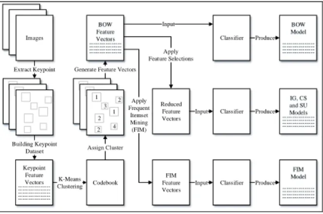
In this section, we will describe our proposed method, which involves how we generate BOW feature vectors, the process of extracting FIM descriptors from BOW, and finally, how we combine FIM classifiers with other classifiers as inputs to the ensemble methods. As previously stated, we use the spatial pyramid due to its capabilities in generating features that can give different representations for each pyramid level. Apart from that, we also believe that this approach can provide features representations that have more discriminative power in recognizing images compared to other approaches. In addition, we also deploy two more image segmentation techniques, namely row and column. A row image partition is a scheme that divides an image horizontally into two partitions while the column image partition scheme will divide an image vertically. Figure 2 shows a block diagram on how models for BOW, IG, SU, CS and FIM are generated. There are three main stages, namely the vector quantisation, feature selection and classification.
Codebook Keypoint Feature Vectors ---Classifier Extract Keypoint Images Building Keypoint Dataset K-Means Clustering Assign Cluster Generate Feature Vectors
Input 2 1 3 2 4 1 2 2 1 3 2 4 1 2 2 1 3 2 4 1 2 Reduced Feature Vectors Apply Feature Selections Classifier FIM Feature Vectors Apply Frequent Itemset Mining (FIM) Input Classifier Input BOW Model ---IG, CS and SU Models ---FIM Model ---Produce Produce Produce BOW Feature Vectors
---Figure 2: Block diagram to generate models
Vector quantisation starts by identifying the keypoints in the images based on SIFT algorithm. Once the keypoints have been identified, the keypoint descriptor is created. After that, a keypoint dataset is build which involves constructing a keypoint dataset that the k-means clustering algorithm will work on. Since we used SIFT as a local feature, each SIFT descriptor has 128 features. These 128 features form a 128-dimensional feature vector which uniquely represents a keypoint. In this step, a keypoint dataset consisting of all
keypoint feature vectors that are extracted from the images is generated. Then, the K-means clustering algorithm is applied to the keypoint feature vectors. Clustering tends to group more similar SIFT descriptors within the same cluster. The K-mean algorithm takes the feature vectors and the number of clusters to generate, k, as input and return a set of centroids. These centroids have the same feature dimension as the keypoint feature vectors. A codebook mapping the cluster numbers and centroids is generated in this stage.
After the codebook is generated, the distance between a keypoint and the centroids are computed. The keypoint is assigned to a centroid to which it is the closest. This assignment is based on the minimum sum of the squared distances between a keypoint and the centroids. However, to simplify the representation, each keypoint is represented by a cluster number rather than its centroid. The distance is computed using the Euclidean distance formula as follows:
k i x S i S i x 1 2 min arg (1)where: x = keypoint feature vector
s = centroid feature vector k = number of clusters to generate
In order to construct BOW feature vectors, a histogram that describes an image is computed by identifying frequencies of cluster numbers in an image using HBOF. For each cluster number w in the codebook C, the histogram of cluster numbers is computed as follows:
n i x s dist w if otherwise i c w HBOF 1 )) , ( ( min arg 1 0 ) ( (2)where: n = number of keypoints in an image
xi = feature vector computed at keypoint i s = cluster centroid
In the feature selection stage, three different approaches are applied: (1) To classify BOW feature vectors without going through any feature selection processes. (2) BOW feature vectors will be applied with IG, SU and CS. (3) Frequent itemsets in the BOW feature vectors are identified and a new FIM feature vector will be generated. The resulting feature vectors, after going through the feature selection process using the same feature descriptors as BOW but the size has been reduced. The selected feature descriptors depends on the feature selection algorithm. However, the new feature descriptors are created when the original BOW feature vectors are applied to the frequent itemset mining.
We use a small example to illustrate how the FIM feature descriptors are extracted from the BOW feature vectors as shown in table 1 and table 2. Refer to table 1, the set of features are cluster 1 (C1), cluster 2 (C2), cluster 3 (C3), cluster 4 (C4) and cluster 5 (C5) while the number of images are 5.
Assuming that the support applied is 50%. At first, the frequencies or support of each feature are counted separately. In this case, the frequency is 0 if the value of the data is 0 (absence in the image) and 1 if the value is a positive integer (presence in the image). At level 1 support, cluster 1 is considered not frequent as it only appears on image 2 and image 4. Since the support of cluster 1 (40%) is below the
minimum support (50%), it is removed from the frequent item lists and will not be included as a candidate of the frequent item lists for level 2 support. Therefore, the frequent item lists at level 1 support are cluster 2 to cluster 5 (written in bold) that have supports greater or equal to the minimum support. The next step is to generate a list of 2-pairs of the frequent items.
Table 1
Example of BOW Feature Vectors
Image No. C1 C2 C3 C4 C5 1 0 18 5 6 17 2 3 13 6 0 0 3 0 0 0 6 1 4 17 11 5 5 19 5 0 0 2 7 0
The candidate of 2-pair frequent items are only selected from a pool of frequent items at level 1 which consists of the sets {C2-C3}, {C2-C4}, {C2-C5}, {C3-C4}, {C3-C5} and {C4-C5}. There are only three 2-pair frequent items at level 2 that meet the minimum support, namely {C2-C3}, {C3-C4} and {C4-C5}. In a similar fashion, the possible 3-pair frequent items at level 3 support are C4}, {C2-C3-C5} and {C3-C4-{C2-C3-C5}. However, the algorithm will end at level 3 support since none of the three 3-pair candidates of frequent item lists generated have met the desired support. Thus, the frequent item lists for all levels consist of the sets {C2}, {C3}, {C4}, {C5}, {C2-C3}, {C3-C4} and {C4-C5} as in table 2, are adopted as FIM feature descriptors.
Table 2
Frequent Items Generated from BOW
Level Features Support
1 C1 40% C2 60% C3 80% C4 80% C5 60% 2 C2-C3 60% C2-C4 40% C2-C5 40% C3-C4 60% C3-C5 40% C4-C5 60% 3 C2-C3-C4 40% C2-C3-C5 40% C3-C4-C5 40%
Referring to figure 2, in the classification stage, after the feature vectors for BOW, IG, SU, CS and FIM are obtained, they can be used to train the classifiers. These feature vectors are represented by m x n matrix where m is the number of images and n is the number of feature descriptors. We employ an SVM algorithm to learn and classify the images. An SVM will find a hyperplane that separates the two classes of data with the widest margin. After all single classifiers are obtained, the ensemble methods will combine the classifiers using three weightage schemes. First is the default weightage scheme, which is a simple weightage scheme where all classifiers have the same weightage value. Second is the linear weightage scheme, where a classifier with better accuracy will be assigned more weight than a worse classifier in a linear fashion. Last is the skew weightage scheme, where a classifier with better accuracy will be assigned a very large weight and a worse classifier is assigned with a very small weight. In the linear and skew weightage schemes, all classifiers are ranked based on their accuracies. We used formula f(x)=x for linear and f(x)=1/x for skew in assigning the weights.
IV. EXPERIMENTS AND RESULTS
In this section, we introduce the datasets used in our experiments, explain the setup and finally, report the results of the two datasets.
A. Dataset
We need creditable datasets to test and compare our proposed method. Building an image spam dataset is difficult because e-mails are personal, especially those with legitimate images. For this reason, many researchers use their personal images or images from Google image engine as their collection of legitimate images. Dredze and SpamArchive are two openly accessible datasets that have been used in our experiments. In our best knowledge, Dredze dataset is the only image spam dataset that has both; spam and legitimate images. There are 3,297 spam and 2,020 legitimate images. Since SpamArchive dataset has spam images only, we combine it with legitimate images from the Dredze dataset. The total number of spam and legitimate images for SpamArchive dataset are 15,090 and 2,020 respectively.
B. Experimental Setup
The SVM algorithm is built from a package called libsvm [28] and the FIM algorithm is obtained from [29]. We applied a maximum angle of 1800 and a Gaussian blur with σ = 1.0
for SIFT. In order to find the optimal cluster, preliminary experiments have been performed where the feature vectors were quantized using a k-mean clustering from k=100 to k=3,000 with the increment of 100 for each run. The best result is obtained at k=2,600 for Dredze and k=2,300 for SpamArchive. As for FIM, we set the minimum support to 0.4.
Three different levels, L0, L1 and L2 were processed for the spatial pyramid. Since Dredze and SpamArchive consist of unbalanced datasets, especially SpamArchive with 13,745 spam and 1,828 legitimate images, we chose 100 repeated random sub-sampling as our validation method. We believe that if the k-fold cross validation is used, the classifier will learn more spam than legitimate. We randomly divided 1,000 images into the training and test sets, with 500 images for each class. The accuracy was calculated by averaging the results from all 100 runs.
The Support Vector Machines (SVM) are perhaps the most extensively used machine learning algorithms. In our experiments, an SVM classifier is used to train the binary classification since both datasets have only two classes, spam and legitimate. We chose Java Software LibLinear 1.92, an SVM classifier with a linear kernel because most researchers have reported that LIBLINEAR is very efficient for a large-scale problems training.
C. Results on Dredze Dataset
Table 3 shows the average classification accuracy (%) and standard deviation of the Dredze dataset using five different descriptors on three image partitioning schemes. Experiments were conducted on spatial pyramids, and another two partition schemes, row and column. Before we choose the cluster size, an initial experiment has been run for a multiple cluster size, from 100 to 3000 with an interval of 100. The best performance is achieved at cluster 2,600 with 97.6% accuracy.
Table 3
The Average Classification Accuracy (Mean and Standard Deviation) on Dredze Dataset using single classifiers
Partition
Scheme BOW IG SU CS FIM
L0 97.6± 0.6 97.3± 0.7 97.2± 0.6 97.3± 0.6 95.0± 0.8 L1 97.7± 0.6 97.7± 0.6 97.7± 0.6 97.7± 0.6 95.0± 1.0 L2 97.6± 0.7 97.5± 0.6 97.6± 0.7 97.5± 0.6 94.2± 1.0 Row 97.6± 0.6 97.4± 0.6 97.4± 0.6 97.5± 0.6 94.0± 0.9 Column 97.6± 0.6 97.4± 0.6 97.4± 0.6 97.5± 0.6 94.0± 0.9 Naive 97.6± 0.7 97.7± 0.6 97.6± 0.7 97.6± 0.6 95.0± 1.0
The reported results are based on the 2,600 cluster dataset. The table shows that the BOW approach works better for L0, L2, row and column than any feature selection methods and FIM. However, at L1, all feature descriptors except FIM delivered the best result which is 97.7%. The best result is illustrated in bold characters. As expected, the classification performance is much better when the number of level is increased from 0 to 1, but slightly decreased at L2. This is probably a large number of clusters (2,600 clusters in each partition) which leads to less discriminative descriptors. We believe that BOW already have sufficient information to describe the images. Further analysis was done using the naïve approach by combining all feature vectors (L0-L2) for each descriptor. This approach produced a very large single feature vector because it concatenated all feature vectors from L0 to L2.
Table 4 shows the results when all single classifiers are combined using the ensemble method. As discussed previously, we used three weightage schemes namely default, linear and skew. We also used two combination methods which are the product rule and mean rule. The highest accuracy is achieved using linear weightage scheme with the mean rule as the combination method and the combination of all feature descriptors for all levels (L0 to L2) with accuracy of 98.0%. This result significantly outperformed the best performance of the single classifiers which is at 97.7%.
Table 4
The Average Classification Accuracy (Mean and Standard Deviation) on Dredze Dataset using Ensemble Methods
Default Linear Skew
Level Product Mean Product Mean Product Mean
L0 97.5±0.6 97.5±0.6 97.5±0.6 97.5±0.6 97.5±0.6 97.6±0.6
L1 97.7±0.6 97.7±0.6 97.7±0.6 97.8±0.6 97.7±0.6 97.7±0.6
L2 97.6±0.7 97.6±0.6 97.6±0.7 97.7±0.6 97.6±0.7 97.6±0.6
L0-L2 97.9±0.6 97.9±0.6 97.9±0.6 98.0±0.6 97.9±0.6 97.9±0.6
D. Results on SpamArchive Dataset
Results for SpamArchive is slightly lower than as reported in Dredze. This might be due to large intra-class variations in the SpamArchive dataset. In this case, image variations occur between different images of the same class. Same as Dredze, the results for the initial experiment is achieved at cluster 2,300. Table 5 shows that the highest accuracy is achieved by IG, SU and CS using the naïve approach (bold characters). It shows that the accuracy for each level increases in proportion to the increment in resolution. For all descriptors, the best performance is achieved using the naïve approach.
However, ensemble methods do not improve the result of single classifiers, instead they are reported to have the same accuracy. The best accuracy is 91.3% which is achieved by combining all single classifiers for all levels (L0 to L2), for default and linear weightage scheme and both combination methods. There is a clear trend of increasing in performance
when the ensemble method is applied at a finer resolution. Table 5
The Average Classification Accuracy (Mean and Standard Deviation) on SpamArchive Dataset using single classifiers
Partition
Scheme BOW IG SU CS FIM
L0 89.9±1.1 89.7±1.2 89.6±1.2 89.7±1.1 85.7±1.4 L1 90.5±1.1 90.3±1.1 90.4±1.0 90.4±1.0 87.0±1.5 L2 91.1±1.0 91.1±1.1 91.2±1.1 91.1±1.1 87.2±1.3 Row 90.2±1.2 90.1±1.1 90.1±1.1 90.1±1.1 85.0±1.6 Column 90.2±1.2 90.1±1.1 90.1±1.1 90.1±1.1 85.0±1.6 Naive 91.2±1.0 91.3±1.0 91.3±1.0 91.3±1.0 88.7±1.3 Table 6
The Average Classification Accuracy (Mean and Standard Deviation) on SpamArchive Dataset using Ensemble Methods
Default Linear Skew
Level Product Mean Product Mean Product Mean
L0 90.0±1.2 90.0±1.2 90.0±1.2 89.8±1.2 90.0±1.2 89.8±1.2
L1 90.6±1.0 90.6±1.0 90.6±1.0 90.3±1.0 90.6±1.0 90.3±1.0
L2 91.1±1.1 91.1±1.1 91.1±1.1 90.4±1.1 91.1±1.1 90.4±1.1
L0-L2 91.3±1.0 91.3±1.0 91.3±1.0 90.9±1.0 91.3±1.0 90.9±1.0
V. CONCLUSION
Two methods were proposed where the FIM techniques were applied in the image partitioning schemes and ensemble methods. BOW feature vectors were created by grouping similar SIFT keypoints using K-Mean clustering. BOW is computed at different multi resolution levels. FIM descriptors were generated from frequent itemsets of BOW feature vectors. This study has found that generally, FIM as single classifiers has acceptable performances. Even though the results using single classifiers show that FIM cannot outperform other classifiers, the achieved accuracies are close compared to the other classifiers. However, the combination of FIM classifiers with other classifiers significantly outperformed the best single classifier for both datasets. The results of this study indicate that FIM descriptors can be a useful input to the ensemble methods.
ACKNOWLEDGMENT
The first author would like to thank Universiti Teknikal Malaysia Melaka (UTeM) and Ministry of Higher Education Malaysia for funding this PhD research.
REFERENCES
[1] F. Gargiulo, A. Penta, A. Picariello, and C. Sansone, “Using Heterogeneous Features for Anti-spam Filters,” in 2008 19th International Conference on Database and Expert Systems Applications, 2008, pp. 670–674.
[2] P. Hayati and V. Potdar, “Evaluation of spam detection and prevention frameworks for email and image spam,” in Proceedings of the 10th International Conference on Information Integration and Web-based Applications & Services - iiWAS ’08, 2008, p. 520.
[3] M. Das, A. Bhomick, Y. J. Singh, and V. Prasad, “A modular approach towards image spam filtering using multiple classifiers,” in 2014 IEEE International Conference on Computational Intelligence and Computing Research, 2014, pp. 1–8.
[4] G. Fumera, I. Pillai, and F. Roli, “Spam Filtering Based On The Analysis Of Text Information Embedded Into Images,” J. Mach. Learn. Res., vol. 7, pp. 2699–2720, 2006.
[5] D. Yamakawa and N. Yoshiura, “Applying Tesseract-OCR to detection of image spam mails,” 2012 14th Asia-Pacific Netw. Oper. Manag. Symp., vol. 1, pp. 1–4, Sep. 2012.
[6] A. Attar, R. M. Rad, and R. E. Atani, “A survey of image spamming and filtering techniques,” Artif. Intell. Rev., vol. 40, no. 1, pp. 71–105,
Aug. 2011.
[7] M. Dredze, R. Gevaryahu, and A. Elias-Bachrach, “Learning Fast Classifiers for Image Spam,” in Proceedings of the Fourth Conference on Email and Anti-Spam (CEAS’ 07), 2007, pp. 487–493.
[8] H. B. Aradhye, G. K. Myers, and J. A. Herson, “Image analysis for efficient categorization of image-based spam e-mail,” in Eighth International Conference on Document Analysis and Recognition (ICDAR’05), 2005, no. c, p. 914–918 Vol. 2.
[9] D. G. Lowe, “Object recognition from local scale-invariant features,” Proc. Seventh IEEE Int. Conf. Comput. Vis., vol. 2, no. [8, pp. 1150– 1157, 1999.
[10] J. Chen, L. Zhang, and Y. Lu, “Application of Scale Invariant Feature Transform to Image Spam Filter,” in 2008 Second International Conference on Future Generation Communication and Networking Symposia, 2008, pp. 55–58.
[11] X. Feng, R. Zheng, H. Jin, and L. Zhu, “Weighting scheme for image retrieval based on bag-of-visual-words,” IET Image Process., vol. 8, no. 9, pp. 509–518, Sep. 2014.
[12] L.-J. Zhao, P. Tang, and L.-Z. Huo, “Land-Use Scene Classification Using a Concentric Circle-Structured Multiscale Bag-of-Visual-Words Model,” IEEE J. Sel. Top. Appl. Earth Obs. Remote Sens., vol. 7, no. 12, pp. 4620–4631, Dec. 2014.
[13] L. Rokach, “Ensemble-based classifiers,” Artif. Intell. Rev., vol. 33, no. 1–2, pp. 1–39, Nov. 2009.
[14] B. Fernando, E. Fromont, and T. Tuytelaars, “Effective Use of Frequent Itemset Mining for Image Classification,” in 12th European Conference on Computer Vision, 2012, pp. 214–227.
[15] G. Csurka, C. R. Dance, L. Fan, J. Willamowski, and C. Bray, “Visual Categorization with Bags of Keypoints,” in ECCV International Workshop on Statistical Learning in Computer Vision, 2004. [16] K. Grauman and T. Darrell, “The pyramid match kernel: discriminative
classification with sets of image features,” in Tenth IEEE International Conference on Computer Vision (ICCV’05) Volume 1, 2005, p. 1458– 1465 Vol. 2.
[17] A. Abdullah, R. C. Veltkamp, and M. A. Wiering, “Spatial Pyramids and Two-layer Stacking SVM Classifiers for Image Categorization: A Comparative Study,” in International Joint Conference on Neural Networks, IJCNN., 2009, pp. 5–12.
[18] A. Abdullah, R. C. Veltkamp, and M. A. Wiering, “Fixed partitioning and salient points with MPEG-7 cluster correlograms for image categorization,” Pattern Recognit., vol. 43, no. 3, pp. 650–662, Mar. 2010.
[19] S. Lazebnik, C. Schmid, and J. Ponce, “Beyond Bags of Features: Spatial Pyramid Matching for Recognizing Natural Scene Categories,” in 2006 IEEE Computer Society Conference on Computer Vision and Pattern Recognition, 2006, vol. 2, pp. 2169–2178.
[20] R. Agrawal, T. Imielinski, and A. Swami, “Mining association rules between sets of items in large databases,” ACM SIGMOD Rec., vol. 22, no. May, pp. 207–216, 1993.
[21] B. U. Maheswari and P. Sumathi, “A Comparative Study of Rule Mining Based Web Usage Mining Algorithms,” Int. J. Sci. Res., vol. 4, no. 11, pp. 2540–2543, 2015.
[22] A. M. Parekh, A. S. Patel, S. J. Parmar, and P. V. R. Patel, “Web usage Mining : Frequent Pattern Generation using Association Rule Mining and Clustering,” Int. J. Eng. Res. Technol., vol. 4, no. 4, pp. 1243– 1246, 2015.
[23] L. C. Wuu, C. H. Hung, and S. F. Chen, “Building intrusion pattern miner for Snort network intrusion detection system,” J. Syst. Softw., vol. 80, no. 10, pp. 1699–1715, 2007.
[24] S. Naulaerts, P. Meysman, W. Bittremieux, T. N. Vu, W. Vanden Berghe, B. Goethals, and K. Laukens, “A primer to frequent itemset mining for bioinformatics,” Brief. Bioinform., vol. 16, no. 2, pp. 216– 231, 2015.
[25] A. Abdullah, R. C. Veltkamp, and M. A. Wiering, “Ensembles of novel visual keywords descriptors for image categorization,” in 2010 11th International Conference on Control Automation Robotics & Vision, 2010, no. December, pp. 1206–1211.
[26] R. Duangsoithong and T. Windeatt, “Relevance and redundancy analysis for ensemble classifiers,” Lect. Notes Comput. Sci. (including Subser. Lect. Notes Artif. Intell. Lect. Notes Bioinformatics), vol. 5632 LNAI, pp. 206–220, 2009.
[27] M. a. Wiering and H. van Hasselt, “Ensemble algorithms in reinforcement learning,” IEEE Trans. Syst. Man, Cybern. Part B Cybern., vol. 38, no. 4, pp. 930–936, 2008.
[28] and C.-J. L. Chih-Wei Hsu, Chih-Chung Chang, “A Practical Guide to Support Vector Classification,” BJU international, vol. 101, no. 1. pp. 1396–400, 2008.
[29] P. Fournier-Viger, “SPMF: A Java Open-Source Pattern Mining Library,” J. Mach. Learn. Res., vol. 15, pp. 3569–3573, 2014.