Convolutional neural networks for efficient object detection on ultra low-power platforms

Università di Bologna

M

ASTER

T

HESIS

Convolutional Neural Networks for Efficient Object Detection on

Ultra Low-Power Platforms

A

Pedro José Pereira Vieito

T

A

Prof. Dr. Luca Benini

Dr. Francesco Conti

S

Dr. Francesc Moll Echeto

Master’s Degree in Electronics Engineering

U

P

C

A

BSTRACT

At the University of Bologna, the Microelectronics Research Group has been working on smart data analytics on ultra-low-power sensors for the past few years. This smart analysis is in many cases based on convolutional neural networks as the fundamental tool to extract features and information out of various raw data streams. Applying these techniques on the acquisition device itself can help reducing data transfer and storage but requires neural network models with small memory footprint and a really constrained computation workload.

This work proposes a software architecture and advanced quantization techniques to obtain image classification models with high accuracy, small size and low memory footprint that can properly work on a power device. The design is specifically tailored to support the low-resolution environment available in the PULP platform, which includes a hardware convolution engine to efficiently compute convolution operations required by neural network models.

C

1INTRODUCTION ... 8

1.1 Description ... 8

1.2 Objectives ... 9

1.3 Content ... 9

2CONVOLUTIONAL NEURAL NETWORKS ... 10

2.1 Neural Networks ... 10 2.2 Structure ... 10 2.3 Layers ... 11 2.3.1 Dense Layer ... 11 2.3.2 Convolutional Layer ... 12 2.3.3 Activation Layer ... 13 2.3.4 Pooling Layer ... 14 2.4 Training ... 14 2.4.1 Loss function ... 14 2.4.2 Optimizer ... 14 2.4.3 Gradient-based learning ... 15 2.4.4 Back-propagation ... 15 2.5 Image Recognition ... 15 2.6 Topologies ... 16 2.6.1 LeNet ... 16 2.6.2 AlexNet ... 17 2.6.3 GoogLeNet ... 17 2.6.4 VGG ... 17 2.6.5 SqueezeNet ... 17

2.7 Deep Learning Software ... 18

2.7.1 Caffe ... 18

2.7.2 Torch ... 18

2.7.4 TensorFlow ... 18 2.7.5 Keras ... 18 3SOFTWARE ARCHITECTURE ... 19 3.1 Description ... 19 3.2 NeuralNetTool ... 20 3.2.1 Features ... 20

3.2.2 Command Line Interface ... 20

3.2.3 Dataset Loader ... 21 3.2.4 Execution Flow ... 21 3.2.5 Interoperability ... 23 3.3 NeuralNetModel ... 24 3.3.1 GenericNet ... 24 3.3.2 Models ... 25 3.4 NeuralNetCore ... 25 4SQUEEZENET DESIGN ... 27 4.1 Introduction ... 27 4.2 Topology ... 27 4.2.1 Strategies ... 27 4.2.2 Fire Module ... 27 4.2.3 Architecture ... 29 4.3 Implementation ... 30 4.3.1 Model Tensor ... 30 4.3.2 Fire Module ... 30 4.3.3 SqueezeNet ... 31 4.3.4 Verification ... 32 4.4 Quantization ... 32 4.4.1 Simulated Quantization ... 33 4.5 Quantization Implementation ... 34 4.5.1 Quantclip Operator ... 34

4.5.2 QuantizedConv2D ... 35

4.5.3 Quantized Fire Module ... 38

4.5.4 QuantizedSqueezeNet ... 39

5EXPERIMENTAL RESULTS ... 42

5.1 Training ... 42

5.1.1 Training Setup ... 42

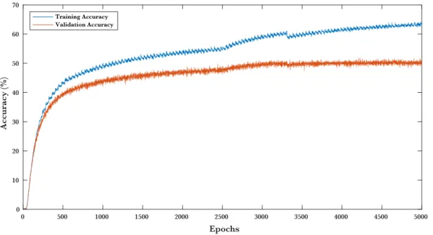
5.1.2 Training Results ... 43

5.2 Model Data Analysis ... 44

5.2.1 Weigh Data Analysis ... 44

5.2.2 Convolution Output Analysis ... 46

5.3 Off-model Quantization ... 47 5.3.1 Quantclip Function ... 47 5.3.2 Kernel Clipping ... 48 5.3.3 Kernel Resolution ... 49 5.4 On-model Quantization ... 49 5.4.1 Kernel Quantization ... 49

5.4.2 Kernel + Input Quantization ... 50

5.4.3 Full Quantization ... 51 5.5 Dynamic Quantization ... 52 5.5.1 Introduction ... 52 5.5.2 Quantize-and-Lock ... 52 5.5.3 Quantize-and-Lock + Custom MSB ... 54 5.5.4 Quantize-while-Train ... 56

5.5.5 Long Duration Quantize-while-Train ... 58

6CONCLUSIONS AND FUTURE DEVELOPMENT ... 60

6.1 Conclusions ... 60

6.2 Future Development ... 60

1

I

1.1

D

At the University of Bologna, the Microelectronics Research Group has been working on smart data analysis on ultra-low-power sensors for the past few years along the entire technological stack, from the acquisition hardware to the software running on microcontrollers. This smart analysis is in many cases based on convolutional neural networks (CNN) as the fundamental tool to extract features and information out of various raw data streams.

The amount of data needed to be transferred from a low-power sensor to the final storage and interfacing device can be greatly reduced by the implementation of this technology. The main limitation of this approach is that the data processing in the low-power device must have an extremely small memory footprint and a really constrained computation workload. This is a big inconveniency when working with CNN, as they require a lot of mathematical operations to execute the model.

Figure 1: The on-device processing approach brings multiple advantages to an acquisition system.

The solution proposed in this work is to select a relatively small CNN model with a good object classification accuracy and adapt it to the hardware constraints of a low-power embedded device such as PULP (Parallel Ultra-Low-Power Platform), a hardware computing platform developed in conjunction by the University of Bologna and ETH Zurich Institute.

On this context, the most important feature of the PULP platform is the presence of a hardware convolution engine (HWCE) to efficiently compute convolution operations (Conti & Benini, 2015) while reducing the power consumption of the device during the model execution. This hardware also imposes some constraints on the structure of the convolutional network, as the HWCE is designed to work with convolution filters of small resolution and size. Therefore, it is critical to ensure that the model is properly adapted to a low-resolution environment and works correctly on it.

On-device processing

Low-Power Adquisition

Device

Low-bandwidth link External Storage and

Interface Low-Power

Adquisition Device

High-bandwidth link required

More resources and storage required

External Storage and

The core of this work was the design of a CNN model with high accuracy, small size and low memory footprint that can properly work with resolution convolutions required by a low-power device.

1.2

O

The main goals of this project were the following:

• Design a software system capable of training, evaluating and fine-tuning a convolutional neural network.

• Ensure this software is scalable from a server with a powerful GPU array to a low-power custom embedded device.

• Select and adapt an existing small and efficient CNN model for image classification.

• Replicate the accuracy of the existing model with our custom training software.

• Retrain the model from scratch, using our own full dataset to achieve similar accuracy to the one of the original model.

• Research, evaluate and apply different strategies to adapt a CNN model to a low-resolution environment similar to one available in a low-power platform.

1.3

C

This work comprises of a total of six chapters. After this brief introduction, the following chapter will present the concept of Convolutional Neural Networks, the process to train CNN models, how they are designed for image classification tasks and the libraries available to implement Deep Learning software.

The third chapter will explain the software architecture we implemented to train, evaluate, fine-tune and test various neural network models with different parameters and topologies.

In the fourth chapter, we will detail the selection and modification of a small neural network model. Also, the structure and topology of the model will be detailed.

The fundamental block of this work is the fifth chapter where we will introduce an extensive description of how we have minimized the model size and adapted it to work with low-resolution convolutions. We will point out the different techniques tried and the experimental results

obtained in each case.

Finally, the last chapter will outline the conclusions drawn from the results of the project,

examining and highlighting the most significant decisions. Possible lines of development will also be mentioned.

2

C

N

N

2.1

N

N

An Artificial Neural Network is a complex computing system inspired in the biological brain structure found on nature. These systems are designed to be trained on a huge number of inputs with known outputs. During this training, the model will learn a pattern allowing it to predict the output of other additional inputs.

Usually this training requires large datasets that have been previously tagged with the interested output feature. During the training phase, the internal parameters of the neural network model are modified, enhancing the accuracy of the model in each iteration. This process must be repeated in batches (epochs) until the model achieves the desired accuracy.

An interesting feature of neural networks is that they are largely input agnostic before the training phase. Thus, one neural network model can be trained and adapted to use in a lot of different tasks. This approach allows neural networks to be implemented in a grand variety of technology areas like computer vision, speech recognition, machine translation, video games or social network filtering where the decision or classification task can be extremely difficult to define based on a limited set of rules or instructions.

2.2

S

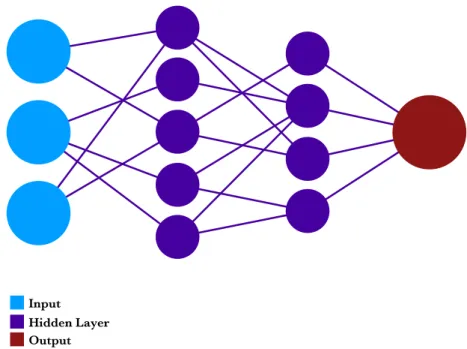
The basic structure of any neural network consists on some inputs, some outputs and several hidden layers which connect the inputs and the outputs.

Figure 2: Schematic structure of a neural network.

These layers are connected through operations which include the trainable parameters that will be tuned during the learning phase. Once the model has been tuned, we can lock the internal parameters and use it for inference, predicting output features on additional input data.

Hidden Layer Output Input

2.3

L

Each connection between nodes inside the network is called a layer. Each layer executes some mathematical operation on its inputs and generates an output. There are a lot of different layer types and the most common ones will be outlined in this section.

2.3.1Dense Layer

Dense layers (also known as fully connected layers) are highly trainable layers which connect each input value to all the outputs with a weighting parameter. Although they are the best way to connect any input size data to a specified output they require large number of trainable

parameters making the model both big and extremely slow to train and execute.

Figure 3: All the connections of a dense layer between four 2×2 images and five simple outputs. This figure shows how dense layers can have a very noticeable size even on small configurations

As all input values are connected to all output values, for ni inputs of size si and no outputs of size

so the model would include the following number of parameters:

𝑑_"#$#%&'&$( = 𝑛₊ ∗ 𝑠₊ ∗ 𝑛_. ∗ 𝑠_.

Equation 1: Number of parameters on a dense layer based on the number and size of the input and output.

The final size of the weight data in the model can be obtained multiplying the number of parameters by the size of the storage data type (typically a float of 32 bits):

𝑑(+/& = 𝑑"#$#%&'&$(∗ 𝑑𝑎𝑡𝑎_𝑠𝑖𝑧𝑒

Equation 2: Storage size of the parameters of the dense layer.

Consequently, for example, a small dense layer connecting four 2×2 images and five outputs the model should include 320 parameters:

𝑑_"#$#%&'&$( = 4 ∗ 4 ∗ 4 ∗ 5 ∗ 1 = 320 𝑝𝑎𝑟𝑎𝑚𝑒𝑡𝑒𝑟𝑠 𝑑_(+/& = 320 𝑐𝑜𝑛𝑛𝑒𝑐𝑡𝑖𝑜𝑛𝑠 ∗ 4 𝑏𝑦𝑡𝑒𝑠 = 1280 𝑏𝑦𝑡𝑒𝑠

Equation 3: Example of the connections and parameter size of a small dense layer.

This example shows how the size of a dense layer can easily exponentially grow when the input nodes and outputs increases. Henceforth, dense layers are unfit for the design of small models

with low memory footprint and we will try to avoid any neural network topology that depends on them.

2.3.2Convolutional Layer

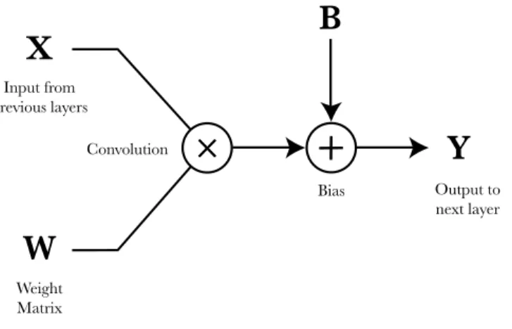
Convolutional layers are the main building block of convolutional neural networks. They are formed by a convolution between the input data and an internal trainable weight matrix (also known as the convolution kernel or filter).

Figure 4: Structure of a convolutional layer; the weight matrix and the bias are its trainable parameters.

Usually after the convolution operation a constant is added to the result. This constant is called the convolution bias and is required to achieve good results during the training of

non-normalized data.

Convolutional layers are great at extracting features from their input, so they are extremely effective in classification tasks like of object detection on images. Using various filters in parallel, convolutional layers can convert spatial information into the feature dimension, extracting each filter a determined classification feature.

Figure 5: Convolution operation applied on an image which extracts some high frequency features.

In contrast to dense layers, convolutional layers store the weight or kernel matrix in a much smaller size, as they share the same kernel parameters for all the input pixels.

X

W

×

×

Y

B

×

×

40 × 40

40 × 40

On a convolutional layer the number of filters, kernel size and convolution parameters determines the output size and the kernel values the effect of the filter applied.

2.3.3Activation Layer

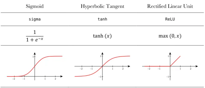
Activation layers are usually intercalated between other type of layers. They are designed to highlight important data values from their input. Historically, there have been three popular activation functions:

Sigmoid Hyperbolic Tangent Rectified Linear Unit

sigma tanh ReLU

1

1 + 𝑒FG tanh (𝑥) max (0, 𝑥)

Table 1: Main activation functions used on neural network models.

The most basic and early activation function is the sigmoid. It takes an input value and squashes it between 0 and 1. This means that large numbers become 1 and negative numbers become 0. The next activation is the hyperbolic tangent function. Like the sigmoid, it saturates the input value, but this time with a zero-centered output, which is typically preferred while training the models.

ReLU has become the most popular activation function is the last years. It acts like a simple thresholder to zero when the value is negative and a pass-through when positive. It has two big advantages in comparison to the previous ones:

• It greatly accelerates the convergence of the model gradient descent (Krizhevsky, Sutskever, & Hinton, 2012), which speeds-up the training phase.

• Compared to other activation functions it can be implemented with an extremely simple mathematical operation, thresholding input values at zero.

The main defect of the ReLU activation function is that it is not robust against large gradients, which can make an activation point stale at a constant zero value. However, this is not typically a problem and ReLU has become the default activation function recommended for most neural networks.

Finally, it is important to note that there are a lot of variations of the ReLU activation function optimized for different use-cases like Leaky ReLU, softmax or ELU.

2.3.4Pooling Layer

Pooling layers are used to reduce the number of data points on a given input. They are non-trainable layers as they simply combine adjacent data points down-sampling the input.

Figure 6: A pooling operation applied to a 40×40 image to output a 16×16 image.

Some convolutional neural networks try to avoid the use of pooling layers by modifying the data size directly during the convolutions, reducing the number of layers and enhancing the efficiency and speed of the model. This result can be achieved configuring each convolutional layer with a stride higher than one, which means that the convolution filter would not be applied to each input pixel, but instead would skip some of them, producing a smaller output.

2.4

T

Training is one of the fundamental steps required to achieve a useful neural network model. All deep learning algorithms must include the following pieces to be properly trained:

• A model with inputs, outputs, connections and trainable parameters.

• A tagged dataset to train and evaluate of the model.

• A cost function that can compute a statistical estimation related to the model accuracy.

• An optimization strategy to update the model parameters while increasing its accuracy.

2.4.1Loss function

As the objective of the training is to maximize the accuracy of the model on a given task, there must be a method to compute the exactness of the model during the process. This is achieved with a cost function (or loss function) which represents a statistical estimation inversely related to the accuracy of the model.

The loss function is a fundamental piece of the learning phase as it provides the tool required to update the model on each iteration of the optimization.

2.4.2Optimizer

The objective of an optimizer is to find the parameter values that minimizes the loss function. To achieve this, multiple algorithms are available:

• Random Search: try multiple random parameters and choose the one that resolves the minimum loss function value. This approach is really simple but will not achieve any

40 × 40

great results due to its random nature.

• Random Local Search: the model would start with some random parameters and then the optimizer would try to update them to obtain better results in the loss function. If a better result is found then it would continue updating the weight parameters in that direction, if not, it would try in another random direction.

• Gradient-Based Learning: this method is the one really used in the practice. It applies an algorithm similar to the random local search optimizer but it also computes the best direction (using the loss function gradient) on which to update the model parameters.

2.4.3Gradient-based learning

The core operation of a gradient-based learning optimizers is defined in the following way, being

𝑤 the previous iteration parameter matrix, 𝑤S _{the updated parameter matrix, 𝛿 the step size and}

𝛻_V(𝐿) the gradient of the loss function over the weight matrix:

𝑤S _{= 𝑤 − 𝛿 ∗ 𝛻} V(𝐿)

Equation 4: Formula to compute the updated weight matrix after each iteration following the gradient direction of the loss function with a defined step size.

This operation is executed in loop, with each iteration updating the model parameters towards the loss function local minimum. That point defines the parameters that produce a local maximum accuracy on the model.

Of course, detecting a local minimum in the loss function does not guarantee that the given point is the absolute minimum, so the optimizer has to deal with various strategies to find a valuable accuracy. These techniques involve modifying the step size of each update to change the path towards the maximum accuracy.

Gradient computation can be a hard task on complex models, as it requires to derive the function in each dimension, so in real Deep Learning software the implementation uses a technique called back-propagation, which is described in the next section.

2.4.4Back-propagation

Back-propagation is a technique used to efficiently compute the loss function gradient. It separates the gradient calculation in parallelizable operations on each model node to propagate back the output error and compute each parameter deviation. Once those error values are computed the optimizer updates the parameters using the step factor previously defined.

2.5

I

R

Convolutional neural networks are a great tool for image recognition and classification. Usually CNN models for image recognition have a common basic structure that we will describe in the following way:

• An input designed for images of a determined size, usually a square of around 200×200 pixels and with 3 color channels. Early CNN models, like LeNet, where designed for smaller input images, like 20×20 pixels with only one channel.

• Some convolutional layers, intercalated with ReLU activations to extract the features of the input image.

• Some pooling layers to reduce the resolution of the convolutional layers outputs.

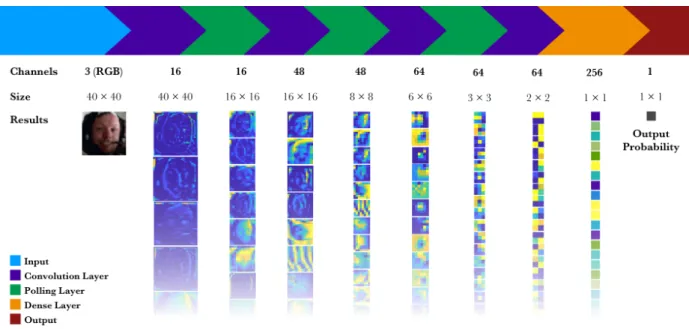
• And finally, a fully connected layer to redistribute the result of the last convolutional layer over the outputs. Typically, the model has as many outputs as image categories, and each output represents the probability that the input image is included in that category. On binary classifier —like cat vs. dog or smiling face vs. not— only one output used, which represents the probability of the image being one of the cases.

The following graph shows an archetypal example of a CNN model for binary classification. Its input is a 40×40 image with three channels, it includes some convolutional, pooling and dense layers and finally, it outputs the probability of the image containing a smile.

Figure 7: Structure and results of each layer of an image recognition convolutional neural network with only one output feature.

2.6

T

2.6.1LeNet

LeNet (LeCun, Bottou, Bengio, & Haffner, 1998) was one of the first neural network models implemented in a commercial product. The design was developed in Bell Labs to allow machines to read hand-written digits. Prior to its design, image recognition software was implemented in two different pieces:

• A Feature Extraction Module which was manually designed to extract some interesting features of the input image like its frequency content or borders.

• A Trainable Classier Module implemented with a model trained with preclassified data. The main innovation of LeNet was that the full implementation could be trained with a preclassified dataset. Both the feature extractor and the classifier were unified in a trainable model. This made possible obtaining a better feature extractor that could be enhanced with the big datasets available.

The second innovation of LeNet was the introduction of convolutional layers in its neural network topology. Convolutional layers allowed for the first time to efficiently extract different image features in what the authors called feature maps.

2.6.2AlexNet

AlexNet (Krizhevsky, Sutskever, & Hinton, 2012) is as CNN model developed in 2012 to achieve high accuracies in complex datasets like ImageNet (1000 categories). Using the ILSVRC-2010 dataset AlexNet achieved an accuracy of 62.5%.

The architecture of AlexNet includes five convolutional layers and three fully-connected layers. The big innovations of AlexNet were the following:

• The introduction of the ReLU non-linearity as an activation function instead of the classical tanh or sigmoid functions, which allowed it to converge quicker.

• Use of complex convolutional layers in a deep neural network model.

2.6.3GoogLeNet

GoogLeNet (Szegedy, Liu, & Jia, 2014) is a convolutional network model designed by Google and winner of the ILSVRC-2014 contest. Its main innovation was the inclusion of a module named Inception designed to intensely reduce the number of parameters in the model (GoogLeNet used only 7% of the parameters required by AlexNet).

Moreover, GoogLeNet reduced the number of trainable parameters by replacing all dense layers in the model by convolutional and pooling layer pairs.

2.6.4VGG

VGG (Simonyan & Zisserman, 2015) is a CNN model designed by the Department of Engineering Science of the University of Oxford. It was the runner-up of the ILSVRC-2014 competition.

Its main contribution was to show that the depth of a neural network (the number of layers) is a critical component to obtain a high accuracy model. Unfortunately, VGG is a really big network, with over 140 million parameters, which is not appropriate for low-power devices.

2.6.5SqueezeNet

SqueezeNet (Iandola, Moskewicz, Ashraf, Han, & Keutzer, 2016) is a CNN model designed to have both small size and high accuracy. The first version of SqueezeNet achieved an accuracy of 57.5% on ImageNet, close to the one accomplished by AlexNet while requiring 50 times less parameters. Moreover, the total size of the SqueezeNet model is under 5 MB allowing for the first time to embed a complex CNN classifier on low-power devices with limited memory.

One of the main innovations of SqueezeNet was the introduction of the Fire module, which could efficiently extract features from the input images with few trainable parameters. Furthermore, to decrease the number of parameters, the model avoids any use of fully connected layers or big kernels on the convolutional layers.

All these features make SqueezeNet an outstanding model for the objective of this work. As explained in the following chapters we used the SqueezeNet topology as the base for our quantized model and its design and implementation is deeply described in the fourth chapter.

2.7

D

L

S

There are multiple Deep Learning libraries available to ease the design, training and execution of convolutional neural network models. This software can be used for several applications like computer vision, machine translation or emotion detection. As running convolutional neural networks require a lot of mathematical operations, Deep Learning software implements low-level libraries which use any hardware acceleration available, like GPUs or the HWCE.

In this section, we briefly detail multiple Deep Learning software libraries available.

2.7.1Caffe

Caffe (Jia, 2013) is one of the most popular and wide-spread deep learning frameworks available. It is written in C++ and includes bindings for different languages like C or Python. Its main benefits are its speed, performance and the huge quantity of models already available. Caffe was created on the Artificial Intelligence Research Department of the University of Berkeley.

2.7.2Torch

Torch (Collobert, 2011) is a scientific computing library with support for machine learning algorithms designed to use the hardware acceleration of the GPU implementing the CUDA API. It is written in C and Lua and its API is exposed through the scripting language LuaJIT.

2.7.3Theano

Theano (Bergstra, 2010) was a low-level mathematical library written in Python. It was written at the LISA lab of the University of Montreal to support rapid development of efficient machine learning algorithms.

Though highly popular on the inception of Deep Learning software, Theano ceased its development after the introduction of competing libraries backed by strong industrial players, like TensorFlow.

2.7.4TensorFlow

TensorFlow (Abadi, 2015) is a modern numerical computation library based on data flow graphs. It is written in C++ and CUDA and includes a Python API. TensorFlow works with

computational graphs that are complex combinations of mathematical operations. They can be easily used to represent a neural network which makes TensorFlow extremely well fitted for Deep Learning applications.

TensorFlow was originally developed by researchers and engineers from Google Brain, the main team in charge of machine learning research at Google.

2.7.5Keras

Keras (Chollet, 2015) is a high level Deep Learning library. It is fully written in Python and has an advanced API to implement neural network models and ease its training and execution. It was developed with a focus on enabling fast experimentation and prototyping.

Keras was designed to allow both Theano and TensorFlow as its mathematical backends so its code is extremely portable on a grand variety of devices and environments.

3

S

A

3.1

D

We selected Keras as the framework on which we would implement the software architecture of the project. The main advantages of Keras is that it has an extensive API, good documentation and community support. Moreover, there are multiple solutions available to import and export models from Keras, which will be required during the development of project.

The most important requirement of the software implementation is that it must run on a wide variety of environments with extremely different resources available. It must also be modular, so multiple models can be easily trained and tested.

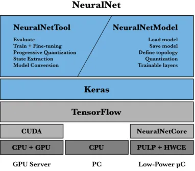
To achieve these goals, the system was designed as three different modules:

• NeuralNetTool: the command line interface to evaluate, train, fine-tune and extract the state of a model.

• NeuralNetModel: the architecture that each model will have to implement to be compatible with NeuralNetTool. Using the same design, different models and topologies can be trained and tested with diverse parameters directly from the command line, speeding up the development and research.

• NeuralNetCore: the low-level module that must implement the hardware acceleration for the math operations needed to evaluate the neural network model on a low-power device.

NeuralNetTool is the interface designed to load the different models implemented using the NeuralNetModel architecture. Under the hood, NeuralNet uses Keras to load the model and execute its training and evaluation. Keras implements TensorFlow as its backend, which will process the low-level mathematical operations with the best hardware acceleration available on the system.

Figure 8: The NeuralNet system architecture. PULP + HWCE

CPU + GPU CPU

TensorFlow

NeuralNetCore Keras

NeuralNet

CUDA

GPU Server PC Low-Power µC

NeuralNetModel NeuralNetTool Evaluate Train + Fine-tuning Progressive Quantization State Extraction Model Conversion Load model Save model Define topology Quantization Trainable layers

3.2

N

N

T

NeuralNetTool is the user interface with the NeuralNet system. It loads the model and executes all the operations requested by the user.

3.2.1Features

NeuralNetTool was designed to support the following operations:

• Loading of large datasets efficiently: training a model requires datasets with

millions of images (for example the ImageNet dataset which we use to train the model has 1000 categories and 10 000 images per category, so 10 000 000 images in total, around 200 GB of data). We implemented a batched generator that can load images using the CPU while the GPU is training the previous batch of images.

• Real-time processing of the dataset images: the dataset images must be processed on-memory before feeding them to the CNN model. We have implemented both the resizing and cropping of the image to specified model input size and the subtraction of the mean pixel of the dataset for a better classification accuracy.

• Evaluation of the model against a given dataset: this operation computes the accuracy of the model over a given validation dataset.

• Training of a model: this operation loads a full training dataset and trains the model during some specified time.

• Fine-tuning of a model: NeuralNet can load a previously trained model and resume the training for all or some layers with modified parameters.

• Model state extraction: this operation can extract all the values at the output of each layer during the inference of a given input image on the model. This is data is very useful to select the best configuration for the quantization of the model.

• Model conversion: NeuralNet can convert a given model to other formats compatible with external analysis tools. This operation supports both HDF5 and Core ML (Apple Inc., 2017) as export formats.

3.2.2Command Line Interface

The command line interface of NeuralNetTool was designed to be extremely flexible and allow the execution of the operations needed both during training, evaluation and analysis of a neural network model.

NeuralNetTool.py - Pedro José Pereira Vieito - 2017

Usage:

NeuralNetTool.py evaluate [options] NeuralNetTool.py train [options]

NeuralNetTool.py progressive_quantization [options] NeuralNetTool.py output_extraction [options]

NeuralNetTool.py coreml_export [options]

Options:

-f=<datasets_folder> Datasets folder [default: DataSets] -d=<dataset> Dataset name [default: ilsvrc12]

-s=<size> Image target size [default: 227] -c=<colormode> Color mode [default: rgb]

-m=<model> Pretrained model to load

-e=<epochs> Epochs to train in train mode [default: 2500] -q=<resolutions> Quantization resolutions k:i:o

--phase=<epochs> Epochs per phase in progressive_quantization --msb=<msb_percentile> Quantization MSB percentile (95, 98, 99.9, 99.99) --neuralnet=<name> NeuralNet name [default: QuantizedSqueezeNet] --gpu=<device> GPU device to use [default: 0]

-r, --relax Add a relaxation phase to the progressive quantization -v Verbosity level

-h, --help Show this help

Code 1: Command line options of the NeuralNetTool.

NeuralNetTool can run the following command operations:

• evaluate: Evaluates the model accuracy against the validation dataset.

• train: Trains model with the training dataset during the specified epochs.

• progressive_quantization: Starts the quantization of a pretrained model following a predefined strategy. We will discuss how we quantized the model and with which techniques on the fifth chapter.

• output_extraction: Dumps an HDF5 file with the state of the outputs of each layer in the neural network during the evaluation of an input image batch.

• coreml_export: Converts and exports a trained model to Core ML format.

Furthermore, NeuralNetTool support a verbose mode (flag --v) which will dump the internal state of the model during the training and show any warnings or notices from the low-level libraries like TensorFlow or CUDA.

3.2.3Dataset Loader

NeuralNetTool was designed to work with large datasets. It can load the ImageNet ILSVRC12 (ImageNet, 2012) dataset with over 10 million images and 1000 categories in less than one minute using Python iterators to preload images on memory in batches in parallel to the GPU operation.

It was implemented with a modified version of the Keras DirectoryIterator class, with support for various channel ordering (RGB vs. BGR, required by some pretrained models from Caffe) and the option to subtract the mean pixel of the dataset, which helps increasing the accuracy of the model during the training.

3.2.4Execution Flow

The NeuralNetTool execution flow is divided in three steps:

• Loads the dataset specified from the Command Line using the DirectoryIterator.

• Loads the selected model and instantiates it with the input size detected from the dataset.

The following simplified Python code exemplifies the execution flow of NeuralNetTool:

... # Initialization code and options parsing

# Dataset loading

train_generator, validation_generator, classes, shape = DataSets.load_dataset(dataset_name, dataset_size,

color_mode=color_mode,

datasets_folder=datasets_folder) ... # Checks that the Dataset is compatible and available

# Model loading neuralnet = NeuralNet(categories=num_classes, input_shape=shape, subtype=train_generator.color_mode, quantization_resolutions=quantization_resolutions, quantization_msb= quantization_msb))

ongoing_model = "ModelData/NeuraNetTool_{}_Ongoing.h5".format(session_uuid) # Functions that define the various operations

def train_model(epochs=1000, initial_epoch=0):

# Executes the training with the options and saves the ongoing model after each epoch neuralnet.model.fit_generator(...)

... # Prints the accuracy and the details of the training

def evaluate_model():

# Executes the evaluation with the command line options scores = neuralnet.model.evaluate_generator(...)

... # Prints the accuracy and the details of the evaluation

def progressive_quantization(epochs_per_phase, relaxation_phase=False): ... # Executes the training while progressively quantizing the layers

def layer_output_extraction():

... # Runs the model and extracts the output from each convolutional layer

def coreml_export():

... # Converts the model to Core ML with coremltools

# Main code

... # Prints details of the model and dataset

# Loads a pretrained model if any available

if neuralnet.trained_model_available() or pretrained_model: load_pretrained_weights()

# Executes the requested command if args["evaluate"]:

evaluate_model() elif args["train"]:

train_model(epochs=int(args["-e"]), initial_epoch=0) elif args["progressive_quantization"]:

evaluate_model()

progressive_quantize_and_lock(int(args["--phase"]), relaxation_phase=args["--relax"]) elif args["output_extraction"]:

layer_output_extraction() elif args["coreml_export"]: coreml_export()

... # Prints the full session details and elapsed time

Code 2: Simplified code structure of NeuralNetTool. 3.2.5Interoperability

The NeuralNet system was designed to be highly portable and platform-independent, hence, it only requires Python, Keras 2 and TensorFlow to run properly. This libraries and software are widely available on any modern computing platform.

Additionally, NeuralNetTool includes support to extract and export data in different formats for analysis and evaluation purposes:

• Supports saving the internal weights of the model in both Hierarchical Data Format (HDF5) and NumPy format. Useful for analysis in numerical computing software like MATLAB.

• Provides the option to extract the output values of each layer during inference in HDF5 for analysis and debugging.

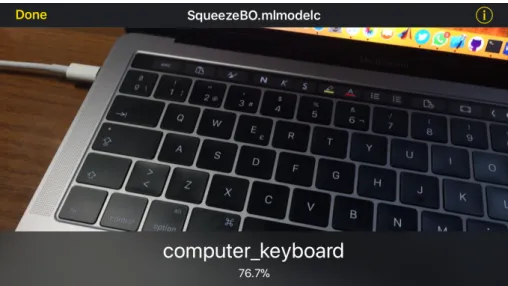
• Includes support for exporting complete models in Core ML format to run them on Apple platforms with full hardware acceleration support.

Figure 9: Model trained with NeuralNet running on DeepVision with hardware acceleration on iOS after exporting it in Core ML.

3.3

N

N

M

Each model that follows the NeuralNetModel architecture inherits its interface from a common basic Python class: GenericNet. This class implements the basic code indispensable for the initialization and data storage of the model and defines the minimum requirements to interoperate successfully with NeuralNetTool.

3.3.1GenericNet

GenericNet subclasses can override the following methods:

• __init__(…): Optional customization of the model initialization.

• create_model(): Required override, the default code will throw an exception. All

GenericNet subclasses are required to store their own neural network topology as a Keras Model instance in their model property.

• compile(): Optional customization of the model optimizer. By default, GenericNet implements a standard SGD optimizer.

The following code shows a simplified version of the GenericNet class implementation:

class GenericNet():

# Common initialization method def __init__(self, categories=1, input_shape=(3, 3, 3), subtype=None, quantization_resolutions=None, quantization_msb=None):

# Autonaming, for example: GenericNet_227x227x3_1000_RGB if not self.name:

self.name = self.__class__.__name__ +

"_" + str("x".join(map(str, input_shape))) +

"_" + str(categories) if subtype:

self.name = self.name + "_" + subtype

# Basic stored properties self.categories = categories self.input_shape = input_shape self.image_channels = input_shape[0] self.image_size = input_shape[-2:] # Advanced quantization properties

self.quantization_resolutions = quantization_resolutions self.quantization_msb = quantization_msb

# After all properties are initialized, GenericNet creates and compiles the model self.create_model()

self.compile()

# Required method. Should save a Keras Model in self.model def create_model(self):

raise Exception("create_model() should be overriden in a GenericNet subclass")

# Compiles the model with the default SGD Optimizer def compile(self):

sgd = SGD(lr=0.04, decay=0.0002, momentum=0.9 , nesterov=True) self.model.compile(optimizer=sgd, loss="categorical_crossentropy", metrics=["accuracy"])

... # Auxiliary methods to load and store the model from disk

Code 3: Simplified implementation of the GenericNetclass. 3.3.2Models

To verify the design of the NeuralNet system, we implemented some neural network models and compared the results with the ones achieved on other software. In particular, we implemented four models with the NeuralNetModel architecture:

• BasicNet: A sample model designed to be easily trained. This model includes two input convolution layers, two output dense layers and a pooling layer in the middle. It can quickly achieve good accuracies —up to 60%— on simple datasets like CIFAR-10 (32×32 images of 3 channels classified in 10 categories). Unfortunately, the use of 2 dense layers implies an extremely huge number of trainable parameters and a big model size — 17 MB, which is huge for CIFAR-10.

• LeNet: The most traditional convolutional neural network. It was designed for character recognition. After training it with the MNIST dataset (16×16 images of black and white hand-written digits from the 0 to 9) we achieved an accuracy of 98.49% with a model size of 5 MB.

• SqueezeNet: A modern small and efficient neural network with high accuracy. This model was replicated using the Keras API following the official description. The topology and architecture of this model will be described in detail in the next chapter.

• QuantizedSqueezeNet: A convolutional neural network based on SqueezeNet with quantized convolutions support to adapt a full-resolution model to a low-resolution environment like the Hardware Convolution Engine of the PULP platform. The design, implementation and evolution of this model is explained in following chapters.

3.4

N

N

C

NeuralNetCore is the piece of software that must forward all the convolution operations executed by the TensorFlow framework to the Hardware Convolution Engine provided by the PULP

platform. This software is not yet implemented, but its purpose is replaced on other platforms with the hardware acceleration provided by the CUDA framework.

Finally, on platforms that do not support neither of those technologies, TensorFlow can downgrade to direct CPU computation.

4

S

N

D

4.1

I

We chose SqueezeNet as our base neural network model due to its efficient topology and small size (Iandola, Moskewicz, Ashraf, Han, & Keutzer, 2016). Its model weight data is around 5 MB and its accuracy on the ImageNet ILSVRC12 dataset is around 57.5%, extremely high for its size and number of parameters. For these properties, it is a great choice for a low-power and memory constrained platform like PULP.

Moreover, SqueezeNet was designed to require a lot of convolution operations with small size kernels (1×1 and 3×3) with non-unity strides to avoid pooling layers. This design aligns perfectly with our low-resolution HWCE. Unfortunately, SqueezeNet was designed to be trained with single-precision floating-point parameters (32-bit) thus, it will require some adjustments to adapt it to a low-resolution environment. We will describe some strategies and their results in the next chapter.

The following sections describe the original SqueezeNet design, our implementation and the modifications required to simulate a low-resolution environment.

4.2

T

4.2.1Strategies

The original designers of SqueezeNet identified three main strategies to minimize the number of parameters required by the model:

• Replace 3×3 filters with 1×1 filters: They chose to implement 1×1 filters whenever possible as this kernel is 9 times smaller than the 3×3 one.

• Decrease the number of channels before a 3×3 filter: As the number of

parameters grows proportionally to channels of the convolutional layer input is critical to reduce them before any convolution with a 3×3 kernel.

• Downsample in the last layers of the network: As described in the second chapter, modern CNN models use convolutional layers with a stride higher than one instead of pooling layers to downsample the input data. Delaying that downsampling until the last layers has been found to lead to better accuracy on classification models (He, Zhang, Ren, & Sun, 2015).

With the first two strategies aimed at reducing the number of parameters of the model and the last one to enhance the accuracy of model the designers, created the basic piece of the

SqueezeNet model, the Fire module.

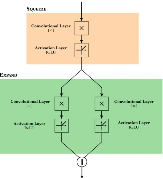
4.2.2Fire Module

In neural network terminology, a module is a group of basic layers that are used as a building block to create a model. The SqueezeNet model includes 10 Fire modules intercalated with some pooling layers. Each Fire module is comprised of 3 convolutional layers, each one followed by a ReLU activation layer. The input of the Fire module is fed into the first convolutional layer with a 1×1 filter followed by its ReLU activation layer. This initial group is called Squeeze layer of the

with a 1×1 filter and other with a 3×3 filter, each one followed by their ReLU activation layer. This group of 2 convolutional layers and 2 activations in parallel is called the Expand layer. Finally, both results are merged into a concatenation producing the output result of the Fire

module.

The following schematic shows the structure of the Fire module, with the Squeeze and the Expand

layers clearly separated.

Figure 10: Internal structure of the Fire module.

The Fire module implements the first strategy of the SqueezeNet team, using two 1×1 kernels and only one 3×3 filter. Both the Squeeze and the Expand groups have some hyperparameters that can be tuned during the design of the network. In particular, each convolution can have a specified number of filters applied to its input: 𝑠_Y×Y, 𝑒_Y×Y and 𝑒_[×[.

Convolutional Layer 1×1

×

×

×

×

×

×

Following the second strategy, the number of filters in Squeeze group should be less than the ones in the Expand one:

𝑠_Y×Y < 𝑒_Y×Y+ 𝑒_[×[

This way the Squeeze convolution will reduce the number of output channels available as input to the 3×3 convolution, helping to reduce the number 3×3 filters which account for the vast

majority of the Fire module trainable parameters.

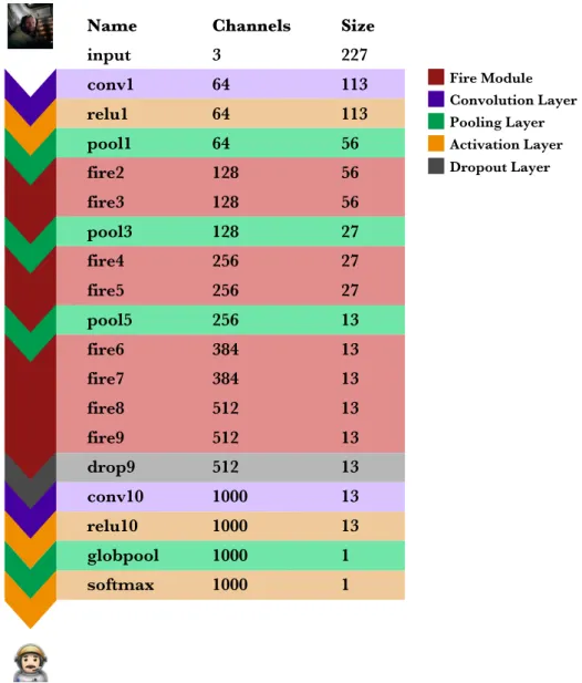
4.2.3Architecture

The SqueezeNet neural network model is designed to have 227×227 images with 3 channels as input and 1000 category probabilities as output.

Figure 11: Structure of the full SqueezeNet neural network.

The first layer of SqueezeNet is the initial convolutional layer, followed by its ReLU activation and a pooling layer. These three layers convert the input image (3×227×227) on 64 images of 56×56 pixels. The process of downsampling and converting the spatial information on feature

Activation Layer Pooling Layer Convolution Layer Dropout Layer Fire Module Name input conv1 relu1 pool1 fire2 fire3 pool3 fire4 fire5 pool5 fire6 fire7 fire8 fire9 drop9 conv10 relu10 globpool softmax Channels 3 64 64 64 128 128 128 256 256 256 384 384 512 512 512 1000 1000 1000 1000 Size 227 113 113 56 56 56 27 27 27 13 13 13 13 13 13 13 13 1 1

resolution (channels) in SqueezeNet is very gradual and performed by the first Fire modules of each pair (fire2, fire4, fire6, fire8).

Following all the Fire modules and before the last convolutional layer there is a dropout layer. This layer is only active during training and it is designed to nullify a specified percentage of its input values. SqueezeNet defines that 50 percent of the values should be dropped. This type of layer is implemented to avoid overfitting the model during training — feeding so many data that the model only learns to classify the training set, not general images.

The last feature extractor of the network is a convolutional layer (conv10) which outputs the 1000 categories fed through a Global Average Pooling (globpool), which averages each one of the 1000 13×13 matrices to its mean value.

The final layer is a softmax, a special activation function which converts any k-dimensional vector of real values to a k-dimensional vector with values in the range [0, 1] that add up to 1. This means that the output values can be treated directly as normalized probabilities which is a great feature for an image classifier.

4.3

I

To recreate the SqueezeNet model we followed the Caffe model description available in the official GitHub repository (DeepScale, 2016). We selected the version v1.1 of SqueezeNet which uses 41% of the computation required by the initial version while obtaining the same accuracy. The published Caffe models include two files:

• A caffemodel file which stores the weights after the training in a binary form. We converted this data to an HDF5 file which is loadable by Keras.

• A prototxt file which declares the structure and layers of the model. Using this file and the description from the SqueezeNet paper we recreated the neural network topology on Keras.

The model was implemented as a GenericNet subclass to follow to NeuralNetModel architecture. As SqueezeNet does not require any special initialization or optimizer the SqueezeNet class does only override the create_model() function from GenericNet.

4.3.1Model Tensor

To understand the implementation of the model, it is important to highlight how Keras and TensorFlow compute the values of the model internally. When a new model is build, Keras instantiates a TensorFlow graph that represents the connection between its input and output. This graph, called in TensorFlow terms tensor, includes all the operations done in between the nodes. This approach allows the software to use the tensor both to compute the output for a given input or the gradient while back-propagating the error during the training.

4.3.2Fire Module

The Fire module is the basic building block of the SqueezeNet model. We have implemented this module as a Python function that appends the Fire module operations to an input tensor:

def fire_module(input, squeeze, expand, name="fire"): x = Conv2D(squeeze, (1, 1), padding="valid",

activation="relu",

name=name + "/squeeze1x1")(input) branch_1 = Conv2D(expand, (1, 1), padding="valid", activation="relu",

name=name + "/expand1x1")(x)

branch_2 = Conv2D(expand, (3, 3), padding="same", activation="relu",

name=name + "/expand3x3")(x)

return concatenate([branch_1, branch_2], axis=3, name=name + "concat") Code 4: Function fire_module that appends the Fire module operators to an input tensor.

The fire_module function includes the squeeze and expand parameters to define the number of

Squeeze and Expand filters applied on each module of the SqueezeNet neural network. 4.3.3SqueezeNet

Using the fire_module function and the built-in Keras layers, we defined the SqueezeNet class with the following Python code:

class SqueezeNet(GenericNet): def create_model(self):

def fire_module(input, squeeze, expand, name="fire"): ... # Code 8 snippet.

input = Input(shape=self.input_shape)

x = Conv2D(64, (3, 3), strides=(2, 2), activation="relu", name="conv1")(input) x = MaxPooling2D(pool_size=(3, 3), strides=(2, 2), name="pool1")(x)

x = fire_module(x, squeeze=16, expand=64, name="fire2") x = fire_module(x, squeeze=16, expand=64, name="fire3")

x = MaxPooling2D(pool_size=(3, 3), strides=(2, 2), name="pool3")(x) x = fire_module(x, squeeze=32, expand=128, name="fire4")

x = fire_module(x, squeeze=32, expand=128, name="fire5")

x = MaxPooling2D(pool_size=(3, 3), strides=(2, 2), name="pool5")(x) x = fire_module(x, squeeze=48, expand=192, name="fire6")

x = fire_module(x, squeeze=48, expand=192, name="fire7") x = fire_module(x, squeeze=64, expand=256, name="fire8") x = fire_module(x, squeeze=64, expand=256, name="fire9") x = Dropout(0.5, name="drop9")(x)

x = Conv2D(self.categories, (1, 1), activation="relu", name="conv10")(x) x = GlobalAveragePooling2D()(x)

out = Activation("softmax", name="loss")(x) self.model = Model(inputs=input, outputs=out)

Code 5: Python code that defines the SqueezeNetclass.

The model definition is done on the create_model function from its superclass, GenericNet, making the model compatible with the NeuralNetModel architecture.

4.3.4Verification

Once we had designed the implementation, we verified that it worked properly with the pretrained weight data. After loading the official pretrained weight model, we got a 56.9% accuracy on the ILSVRC12 verification dataset. The SqueezeNet authors state that their pretrained model has a 57.8% accuracy, so the small difference could be sourced in the unique implementation of the various algorithms used by Keras and Caffe internally. As these results were very similar, we established that the model had been correctly ported to Keras.

There are some important notes to highlight about model conversion from Caffe to Keras:

• Caffe loads the dataset images in BGR channel order instead of the universal RGB. This implies that the dataset loader of the Keras implementation must be able to swap the channels of the images while loading them from disk.

• The SqueezeNet model published by the authors was trained on a dataset with the ImageNet ILSVRC12 mean pixel subtracted. This requires the dataset loader to apply the same transformation when loading the verification images.

Avoiding the mean pixel subtraction reduces the verified accuracy of the model to 36.5% and ignoring the channel swapping to 16.4%. The transformations applied to the training dataset are extremely important to be consistently repeated on other external inputs like the verification dataset, as the model has been biased to classify images which include these transformations.

4.4

Q

Because the objective of this work is to obtain a model designed for low-resolution convolutions, we had to implement some functions that allowed the simulation of that environment. These functions will have to quantize the inputs, execute the convolution, quantize the output and forward the result to the next layer, simulating a Hardware Convolution Engine.

Training the model with these low-resolution constrains implies that all the weight parameters applied to convolutions can be stored on-disk with the reduced resolution without varying the resulting accuracy. For example, after quantizing and training the model with 16-bit resolution values instead of 32-bit float we could save up to 50% of store space without any loss on the accuracy. This property of quantized models must be balanced with the fact that low-resolution convolutions on neural networks require more complex and time-consuming training methods.

4.4.1Simulated Quantization

The implementation of those low-resolution convolutions on the model was accomplished by creating a new NeuralNetModel called QuantizedSqueezeNet and a subclass of the built-in Keras Conv2D layer with quantization support, QuantizedConv2D. The main code of the

QuantizedSqueezeNet class is similar to SqueezeNet but replacing each instance of Conv2D by a QuantizedConv2D.

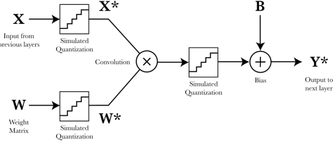
QuantizedConv2D was designed to be completely configurable. Both the bit resolution and the most significant bit of the input, kernel and output can be independently tuned. The layer also includes the option to bypass the quantizations, behaving exactly like a Conv2D layer.

Figure 12: Structure of the QuantizedConv2D layer.

The core of this new layer is the function block that simulates a quantization of the inputs and output of the convolution. This operation must clip the values around a specified range and quantize the result. The clipping range is given by the most significant bit (MSB) of the quantization configuration:

𝐴 = ±2_`a

Equation 5: Formula to compute the amplitude of the clipping range from the specified MSB.

The resolution of quantization can be calculated from this result and the number of bits, 𝑛:

𝑞 =2 ∗ 𝐴

2c =

2_`adY

2c

Equation 6: Relation between the quantization resolution, MSB and number of bits of the parameter.

The complete quantization operation would proceed the following way. First, it computes amplitude of the clipping boundaries:

𝐴 = 2_`a

Equation 7: Obtaining the clipping amplitude from the MSB parameter.

X

W

×

×

X*

W*

Y*

B

×

×

Then, the quantization resolution:

𝑞 =2 ∗ 𝐴 2c

Equation 8: Computing the quantization resolution from the amplitude and the number of bits.

And with the amplitude, it can get the clipped value, 𝑥_e, of the input, 𝑥:

𝑥_e = min(max(𝑥, −𝐴), 𝐴)

Equation 9: Clipping the input to the amplitude boundaries.

Finally, it will compute the output by dividing the clipped value between the quantization resolution, flooring the result and multiplying again by the resolution to recover the quantized value, 𝑥_g:

𝑥_g = 𝑥e

𝑞 ∗ 𝑞

Equation 10: Quantizing the clipped value with the computed resolution.

4.5

Q

I

4.5.1Quantclip Operator

To implement these equations, we defined a function called quantclip that receives an input tensor, the MSB and resolution parameters and returns an extended tensor with the quantization operations appended to it. To add these operations to the input tensor, we had to implement it using the basic built-in operators from TensorFlow and Keras the following way, being x the input tensor, msb the most significant bit binary value (0 would mean that the MSB value is 20₎

and nbits the resolution of the quantization:

from keras import backend as K import tensorflow as tf

def quantclip(x, msb, nbits): # Amplitude

amplitude = 2 ** msb # Clipping

x = K.clip(x, -amplitude, amplitude) # Resolution (for 2's complement)

q = tf.constant(float(2 * amplitude) / float(2 ** nbits)) # Quantization

y = tf.scalar_mul(q, tf.floordiv(x, q)) return y

Code 6: Python code that defines a function that appends the quantization operations to the output of a tensor using Keras and TensorFlow operators.

The previous code works properly when a tensor is fed with an input value, but will fail while computing its gradient. This is sourced in the definition of the floordiv operator in TensorFlow, which returns None as its constant gradient. While this behavior can be opportune in some cases, as the real gradient of the floor operation is usually 0 or not defined, during back-propagation this result breaks the gradient computation. It is interesting to note that this incompatibility is somewhat similar to one found in Binarized Neural Networks, which apply a binarization function to the values of the model (Courbariaux, Hubara, Soudry, El-Yaniv, & Bengio, 2016). To solve this restriction, we applied a solution similar to the referenced case, overriding the floor function gradient with the Identity case:

from keras import backend as K import tensorflow as tf

def quantclip(x, msb, nbits): # Amplitude

amplitude = 2 ** msb # Clipping

x = K.clip(x, -amplitude, amplitude) # Resolution (for 2's complement)

q = tf.constant(float(2 * amplitude) / float(2 ** nbits))

# Quantization d = tf.div(x, q)

# Overriding the gradient value of the Floor operator

with tf.get_default_graph().gradient_override_map({"Floor": "Identity"}): f = tf.floor(d)

# Computing the output

y = tf.scalar_mul(q, tf.floordiv(x, q)) return y

Code 7: Extended Python code that defines a function that appends the quantization operators to an input tensor and supports the computation of gradients.

4.5.2QuantizedConv2D

The quantclip function is the main building block to convert a basic Conv2D layer into QuantizedConv2D. We achieved this by subclassing Keras Conv2D class and modifying its __init__() and call() functions.

The initialization function was extended to include all the configuration parameters requested by the customizable quantclip operator (quantization_resolutions, quantization_msb), an option to bypass the quantization (quantization_enabled) and a parameter to extract the convolution raw data before the activation and bias (perform_extraction).

quantization_resolutions, quantization_msb, quantization_enabled=True, perform_extraction=False, **kwargs): self.quantization_enabled = quantization_enabled self.quantization_resolutions = quantization_resolutions self.quantization_msb = quantization_msb self.perform_extraction = perform_extraction

super(QuantizedConv2D, self).__init__(filters, kernel_size, **kwargs) ...

Code 8: QuantizedConv2Dinitialization code with the extended parameters.

The quantization_resolutions and quantization_msb parameters are Python lists with 3 values that store the resolution and MSB of the convolution kernel, input and output. For example, the following code initializes a QuantizedConv2D layer with a 16-bit kernel, 8-bit input and 6-bit output with all MSB representing 20_.

num_filters = 64 kernel_size = (3, 3) quant_res = [16, 8, 6] quant_msb = [0, 0, 0]

myQuantizedLayer = QuantizedConv2D(num_filters, kernel_size, quant_res, quant_msb) Code 9: Python code that instantiates a QuantizedConv2D layer.

The second modification required in QuantizedConv2D is to add the quantclip operator to the call() function, which is ran while Keras creates the tensor of the model. The default

implementation of Conv2D uses its internal superclass _Conv to execute the following code that appends a 2-dimensional convolution, a bias and an activation function on the input:

def call(self, inputs): outputs = K.conv2d( inputs, self.kernel, strides=self.strides, padding=self.padding, data_format=self.data_format, dilation_rate=self.dilation_rate) if self.use_bias: outputs = K.bias_add( outputs, self.bias, data_format=self.data_format) if self.activation is not None:

return self.activation(outputs) return outputs

Code 10: Simplified code from the internal _Codelayer class of Keras (Chollet, 2015).

Our implementation redefines this function, maintaining the basic structure and adding the quantization of the input, kernel and output around the k.conv2d() function with the output extraction support:

class QuantizedConv2D(Conv2D): def __init__(...):

... # Code 8 snippet.

def quantclip(self, x, msb, nbits): ... # Code 7 snippet.

def call(self, inputs): kernel = self.kernel if self.quantization_enabled: kernel_bits = self.quantization_resolutions[0] input_bits = self.quantization_resolutions[1] output_bits = self.quantization_resolutions[2] kernel_msb = self.quantization_msb[0] input_msb = self.quantization_msb[1] output_msb = self.quantization_msb[2]

# Quantization of the input and kernel

inputs = self.quantclip(inputs, input_msb, input_bits) kernel = self.quantclip(kernel, kernel_msb, kernel_bits) outputs = K.conv2d( inputs, kernel, strides=self.strides, padding=self.padding, data_format=self.data_format, dilation_rate=self.dilation_rate) if self.quantization_enabled: # Quantization of the output

outputs = self.quantclip(outputs, output_msb, output_bits)

if not self.perform_extraction: if self.use_bias:

outputs = K.bias_add( outputs,

self.bias,

data_format=self.data_format) if self.activation is not None: return self.activation(outputs) return outputs

Code 11: Code that defines the QuantizedConv2D class with the main changes with Conv2D highlighted. 4.5.3Quantized Fire Module

We updated the fire_module function to implement QuantizedConv2D instead of Conv2D and to support the output extraction:

def fire_module(input, squeeze, expand,

quantization_resolutions, quantization_msb, quantization_enabled, perform_extraction=False, name="fire"): x = QuantizedConv2D(squeeze, (1, 1), padding="valid", activation="relu", name=name + "squeeze1x1", quantization_enabled=quantization_enabled, quantization_resolutions=quantization_resolutions, quantization_msb=quantization_msb, perform_extraction=perform_extraction)(input)

# In Fire layers the output extraction is performed after the first # Squeeze convolution which constrains the result of the full layer

if perform_extraction: return x

else:

branch_1 = QuantizedConv2D(expand, (1, 1),

padding="valid", activation="relu", name=name + "expand1x1", quantization_enabled=quantization_enabled, quantization_msb=quantization_msb, quantization_resolutions=quantization_resolutions)(x)

branch_2 = QuantizedConv2D(expand, (3, 3),

padding="same",

activation="relu",

name=name + "expand3x3",

quantization_msb=quantization_msb,

quantization_resolutions=quantization_resolutions)(x)

return concatenate([branch_1, branch_2], axis=3, name=name + "concat")

Code 12: Fire module function adapted with quantization and extraction support. 4.5.4QuantizedSqueezeNet

The QuantizedSqueezeNet class follows the NeuralNetModel architecture in a similar way as SqueezeNet does, but replacing all the instances of Conv2D layers with QuantizedConv2D and adding the option to extract the model tensor output after any convolution.

The following Python code shows the main structure of the QuantizedSqueezeNet class with the extended create_model() method and two additional functions:

• The quantize(level) function quantizes all QuantizedConv2D layers up to the specified level, being 1 only the conv1 layer quantized, 10 all layers quantized and 0 no layers quantized.

• The trunk_at_layer(extraction_level, quantization_level) method trunks the model tensor at the specified QuantizedConv2D layer level with the quantization defined. This method is required for the output extraction mechanism of NeuralNetTool, useful to find the best quantization parameters.

class QuantizedSqueezeNet(GenericNet):

# Quantization Support def quantize(self, level):

self.create_model(quantization_level=level) self.compile()

# Output Extraction Support

def trunk_at_layer(self, extraction_level, quantization_level=10):

self.create_model(quantization_level=quantization_level, extraction_level=extraction_level) self.compile()

def create_model(self, quantization_level=10, extraction_level=11): def fire_module(...):

... # Code 12 snippet.

if self.quantization_resolutions is None or self.quantization_msb is None:

quantization_level = 0 # Do not quantize without quantization parameters

input = Input(shape=self.input_shape)

x = input # Required for input extraction (extraction_level == 0)

if extraction_level >= 1:

x = QuantizedConv2D(64, (3, 3), strides=(2, 2), padding="valid", name="conv1", activation="relu", quantization_enabled=(quantization_level >= 1), quantization_resolutions=self.quantization_resolutions, quantization_msb=self.quantization_msb[0], perform_extraction=(extraction_level == 1))(input) if extraction_level >= 2:

x = MaxPooling2D(pool_size=(3, 3), strides=(2, 2), name="pool1")(x) x = fire_module(x, fire_id=2, squeeze=16, expand=64,

quantization_enabled=(quantization_level >= 2),