Georgia Southern University
Digital Commons@Georgia Southern
Biostatistics Faculty Publications
Biostatistics, Department of
12-18-2015
Correction of Verication Bias using Log-Linear
Models for a Single Binaryscale Diagnostic Tests
Haresh Rochani
Georgia Southern University
Hani M. Samawi
Georgia Southern University
Robert L. Vogel
Georgia Southern University
Jingjing Yin
Georgia Southern University
Follow this and additional works at:
https://digitalcommons.georgiasouthern.edu/biostat-facpubs
Part of the
Biostatistics Commons, and the
Public Health Commons
This article is brought to you for free and open access by the Biostatistics, Department of at Digital Commons@Georgia Southern. It has been accepted for inclusion in Biostatistics Faculty Publications by an authorized administrator of Digital Commons@Georgia Southern. For more information, please [email protected].
Recommended Citation
Rochani, Haresh, Hani M. Samawi, Robert L. Vogel, Jingjing Yin. 2015. "Correction of Verication Bias using Log-Linear Models for a Single Binaryscale Diagnostic Tests."Journal of Biometrics and Biostatistics, 6 (5): 266. doi: 10.4172/2155-6180.1000266
Keywords:
Verification bias; Diagnostic tests; Log-liner models; Missing dataIntroduction
Diagnostic testing in medicine is the process of identifying the patients with and without a particular disease. Accuracy of the diagnostic test is the ability of the test to correctly identify the true disease status of the patient [1]. The test or procedure that determines the true disease status without an error is called the gold standard test. However, even with the existence of a gold standard test, verification for the disease status of each patient may not be obtained due to various reasons such as the invasive nature or too costly gold standard test. For example, the Prostate Specific Antigen (PSA) blood test is used as a screening test for diagnosis of prostate Cancer with a ranging cost from $60 to $80. However, the true diagnosis is generally confirmed by invasive procedures such as prostate biopsy with a ranging cost from $1600 to $1800. Thus patients with a high risk or a prostate screening test positive are more likely to be offered the gold standard test than those with low risk or a negative screening test. Furthermore, the inference about the measures of diagnostic accuracy such as sensitivity, specificity, positive predictive value (PPV) and negative predictive value (NPV) may be biased because individuals who are selected for the gold standard test based on the diagnostic test results are not a random sample [2]. Many authors have referred to this bias as, work-up bias [3] or verification bias [4]. Therefore, in the presence of verification bias, the efficiency of a diagnostic test heavily depends only on those patients whose disease status has been verified. In addition if there is a positive association between patient selection for verification and the test results will produce more bias results [5].
When the true disease status is missing among patients who were not selected for verification, the framework of the missing data mechanism proposed by Rubin can be applied for verification bias correction. If the probability of selecting patients for verification is independent of both observed and unobserved data then missingness in the disease status is considered missing completely at random (MCAR). Missingness in the disease status is considered missing at random (MAR) when the probability of selecting patients only depends on the observed data and it is considered missing not at random (MNAR) when the probability depends on unobserved data [6]. This is most likely to occur when
there is long time lag between the initial test and verification, when there are multiple investigators at various institutions, when the patient population is very heterogeneous or when the disease process is not well understood.
Begg and Greenes [4] proposed a method of verification bias correction for binary diagnostic tests by using Bayes’ theorem under the MAR (i.e. conditional assumption). Zhou [7] derived the maximum likelihood estimators for sensitivity and specificity and their variances under both MAR and MNAR mechanisms. However, under the MNAR assumption, Zhou [7] assumed that two known ratios need to be quantified. Zhou [8] showed that the estimators of PPV and NPV are unbiased and consistent if the probability of selecting patients for disease verification does not depends on the true disease status of the patient (i.e. MAR assumption). Some authors have tried to use multiple imputation methods to correct for verification bias under ignorable missingness [9]. However, the validity of that approach was debated by De Groot et al. [10]. In dealing with multiple diagnostic tests and the presence of covariates, Baker [11] Kosinski and Barnhart [12] suggested regression approaches to deal with the MNAR missing mechanism. However, their models require the use of multiple tests or covariates in order to achieve identifiability. Martinez et al. [13] have tried to address the issue of verification bias in the MNAR setting by using a Bayesian approach with a beta prior distribution. Some authors have tried using Gibbs sampling techniques as a Bayesian approach to correct the verification bias in MNAR estimates [14]. All these available methods require iterative methods to compute the estimates of measures for
*Corresponding author: Haresh Rochani, Assistant Professor, Department of Biostatistics, Jiann-Ping Hsu College of Public Health, Georgia Southern University, Statesboro, GA, 30460, USA, Tel: 912.478.1101; E-mail:
Received October 30, 2015; Accepted December 11, 2015; Published December 18, 2015
Citation: Rochani H, Samawi H, Vogel R, Yin J (2015) Correction of Verication Bias using Log-linear Models for a Single Binary-scale Diagnostic Tests. J Biom Biostat 6: 266. doi:10.4172/2155-6180.1000266
Copyright: © 2015 Rochani H, et al. This is an open-access article distributed under the terms of the Creative Commons Attribution License, which permits unrestricted use, distribution, and reproduction in any medium, provided the original author and source are credited.
Correction of Verication Bias using Log-linear Models for a Single
Binary-scale Diagnostic Tests
Haresh Rochani, Hani Samawi , Robert Vogel and Jingjing Yin Department of Biostatistics, Jiann-Ping Hsu College of Public Health, USA
Abstract
In diagnostic medicine, the test that determines the true disease status without an error is referred to as the gold
standard. Even when a gold standard exists, it is extremely difficult to verify each patient due to the issues of
cost-effectiveness and invasive nature of the procedures. In practice some of the patients with test results are not selected
for verification of the disease status which results in verification bias for diagnostic tests. The ability of the diagnostic
test to correctly identify the patients with and without the disease can be evaluated by measures such as sensitivity,
specificity and predictive values. However, these measures can give biased estimates if we only consider the patients
with test results who also underwent the gold standard procedure. The emphasis of this paper is to apply the log-linear
model approach to compute the maximum likelihood estimates for sensitivity, specificity and predictive values. We
also compare the estimates with Zhou’s results and apply this approach to analyze Hepatic Scintigraph data under the
assumption of ignorable as well as non-ignorable missing data mechanisms. We demonstrated the efficiency of the
Citation: Rochani H, Samawi H, Vogel R, Yin J (2015) Correction of Verication Bias using Log-linear Models for a Single Binary-scale Diagnostic
Tests. J Biom Biostat 6: 266. doi:10.4172/2155-6180.1000266
J Biom Biostat
ISSN: 2155-6180 JBMBS, an open access journal
Page 2 of 5
Volume 6 • Issue 5 • 1000266 verification bias. To demonstrate this idea, define two random variables I and J , each with two levels i = 1,2 and j = 1,2 . Let RJ be the missing
data indicator for variable J, such that RJ= 1 if J is being observed and = 2
J
R , if J is missing. Similarly, let RI = 1 if we observe in variable I.
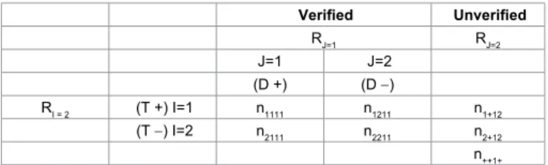
Consider I J× cross-classified Table 3 with total sample size of n++ +1,
each with two levels with one supplemental margin (in the terminology of Dempster and Baker 1992) with cell count nijab. The cell counts with
= = 1
I J
R R is denoted as nij11. The supplemental margin for variable J
when RJ= 2 is denoted by ni+12. In these cases, the symbol ’+’ denotes
the summation over the corresponding index. Furthermore, denote the expected cell counts by λij k1, cell probabilities for I, J, RI and RJ by πijkl
and the marginal probabilities by πij.. for Table 3.
Log-linear models are widely used to analyze contingency tables. Missing data indicators for contingency tables with supplemental margins can be incorporated in log-linear models in the same way as they incorporate the other variables. In terms of λ, the homogenous log-linear model (presence of only two-way interactions) for partially observed one variable is log
( )
µij k1 =λ λ+ I( )i+λJ( )j +λRI(1)+λRJ( )k +λIJ( )ij +λIRI( 1)i +λIRJ( )ik( 1) ( ) (1 )
JRI j JRJ jk R RI J k
λ λ λ
+ + + (1)
Because this is an over parameterized model, we add the
side conditions that the sum of each λ term over each of the
indicated subscripts is zero. For computational purposes, it is convenient to use an alternative parameterization of the model. Let mij≥0, bij≥0 and
∑∑
i jmij(
1+bij)
=n++ +1 suchthat µij11=mij and µij12=m bij ij. In terms of log-linear models
= exp{ ( ) ( ) (1) (1) ( ) ( 1) ( 1) ( 1) ( 1) ij I J RI RJ IJ IRI JRJ JRI JRJ m λ λ+ i +λ j +λ +λ +λ ij +λ i +λ i +λ j +λ j (11)} R RI J λ +
Taking advantage of the side conditions, we can derive the following expression for bij:
= 2exp{ (1) ( 1) ( 1) (11)}
ij RJ IRJ JRJ R RI J
b − λ +λ i +λ j +λ
The detailed derivation can be found in the Appendix. Denote,
(
)
11 1 1 = = 1, = 1| = , = = ij , I J p Pr R R I i J j n µ ++ +(
)
12 2 1 = = 1, = 2 | = , = = ij . I J p Pr R R I i J j n µ ++ +In probabilistic terms, mij and bij can be expressed as follows,
1 1 = ij m n++ +p 12 12 1 2 11 11 1 1 = ij = ij = ij ij ij n p b n p µ µ µ µ ++ + ++ +
For Table 3, the total expected count is
(
)
2 2 2 2 2 2 2 2 2 1 1 11 12 =1 =1 =1 =1 =1 =1 =1 =1 =1 = ij k= ij ij = ij 1 ij i j k i j i j i j m b µ++ +∑∑∑
µ∑∑
µ +∑∑
µ∑∑
+diagnostic accuracy especially under MNAR mechanism. However, by using the log-linear model approach, the explicit solutions for the measures of diagnostic accuracy estimates can be computed by the use of a simple algebraic formula (computationally convenient) under all missing data mechanisms.
In this paper, we provide the log-linear model approach to correct for verification bias in order to compute the estimates of diagnostic measures (i.e. Sensitivity, Specificity, PPV and NPV) under various assumptions of missing data mechanisms. We also confirm by simulations that the estimators are asymptotically unbiased and more efficient than complete cases estimates. In next section, we will show the impact of verification bias by using hypothetical example. The following sections will focus on the method of log-linear models to correct the verification bias for diagnostic measures and comparision with Zhou [7] results. Furthermore, we illustrate the log-linear model approach by application to the Hepatic Scintigraph data.
Impact of Verification Bias
In diagnostic medicine, it is a common practice to refer only patients who are test positives for a gold standard test for disease verification. To illustrate the impact of bias, we considered a hypothetical study of 1000 patients to measure the sensitivity, specificity, PPV and NPV (Tables 1 and 2).
The hypothetical data are summarized in Table 1. If every patient is being referred for verification for the gold standard then the true sensitivity from Table 1 is 0.71. Furthermore, the true specificity, PPV and NPV are 0.87, 0.37 and 0.96 respectively. However, if we consider that only 10% of those who have a test negative result receive the gold standard for verification, then the data are summarized in Table 2. From Table 2, the observed sensitivity, specificity, PPV and NPV are 0.96, 0.4, 0.37 and 0.96 respectively. Overall if positive test results are more likely to receive disease verification, (i.e. MAR) then by using only verified cases, the estimates for sensitivity and specificity are biased, in fact, sensitivity is being overestimated and specificity is being underestimated. However, under the MAR assumption, the estimates of PPV = P D T( + +| ) and NPV = P D T( − −| ) from complete cases are unbiased [8,15,16].
Methodology
Log-linear parameterization
Baker et al.[17] used the homogeneous log-linear model approach to adjust the expected cell counts for a two way table with missing data. We can use the similar approach (BRD model approach) to compute the estimates for measures of diagnostic accuracy correcting for
Verified 2*Unverified 2*Total
-3 D + D −
T + 71 120 0 191
T − 29 780 0 809
1000 Table 1: Hypothetical data.
Verified 2*Unverified 2*Total
-3 D + D −
T + 71 120 0 191
T − 3 78 728 809
1000 Table 2: Hypothetical data with unverified cases.
Verified Unverified RJ=1 RJ=2 J=1 J=2 (D +) (D −) RI = 2 (T +) I=1 n1111 n1211 n1+12 (T −) I=2 n2111 n2211 n2+12 n++1+ Table 3: Two way table with one supplementary margin.
(
)
22 =2| =2.. 12 22 ˆ ˆ = i j = ˆ m ˆ Specificity MCAR m m π +Similarly, the estimates for PPV
(
πˆj i=1| =1..)
and NPV(
πˆj i=2| =2..)
can becomputed from equation 3.
MAR estimates
12 . 11 ˆ = ˆ = ˆi i ij ij i n m n m β + +(
)
(
)
. | .. 2 . =1 ˆ ˆ 1 ˆ = ˆ ˆ 1 ij i i j ij i i m m β π β + +∑
(4)(
)
(
)
. | .. 2 . =1 ˆ ˆ 1 ˆ = ˆ ˆ 1 ij i j i ij i j m m β π β + +∑
(5)From equation 4 the estimates of the Sensitivity and Specificity can be obtained as follows
(
)
(
)
(
11)
1.(
)
=1| =1 11 1. 21 2. ˆ ˆ 1 ˆ = = ˆ ˆ ˆ 1 ˆ 1 i j m Sensitivity MAR m m β π β β + + + + (6)(
)
(
)
(
22)
2.(
)
=2| =2.. 12 1. 22 2. ˆ ˆ 1 ˆ = = ˆ ˆ ˆ 1 ˆ 1 i j m Specificity MAR m m β π β β + + + + (7)can be obtained. Similarly, from equation 5 the estimates of PPV
(
πˆj i=1| =1..)
and NPV(
πˆj i=2| =2..)
can be computed.MNAR estimates
2 . 12 11 =1 ˆ ˆij j= i ˆij= ij j m n m n β +∑
(
)
(
)
. | .. 2 . =1 ˆ ˆ 1 ˆ = ˆ ˆ 1 ij j i j ij j i m m β π β + +∑
(8)(
)
(
)
. | .. 2 . =1 ˆ ˆ 1 ˆ = ˆ ˆ 1 ij j j i ij j j m m β π β + +∑
(9)For Model
( )
β.j , equation 8 provides the estimates of Sensitivityand Specificity as follows
(
)
(
)
(
11)
.1(
)
=1| =1 11 .1 21 .1 ˆ ˆ 1 ˆ = ˆ ˆ ˆ 1 ˆ 1 i j m Sensitivity MNAR m m β π β β + + + +(
)
(
22(
)
.2(
)
)
=2| =2.. 12 2. 22 .2 ˆ ˆ 1 ˆ = = ˆ ˆ ˆ 1 ˆ 1 i j m Specificity MNAR m m β π β β + + + +while equation 9 provides the estimates of PPV
(
πˆj i=1| =1..)
and NPV(
πˆj i=2| =2..)
It is possible to obtain negative maximum likelihood estimates for
. ˆj
β in MNAR model. If any solution is negative (βˆ.1 or ˆ < 0.2 ), the
estimates still can be computed by maximizing the likelihood function by using the limited memory algorithm for constrained optimization Byrd [18]. Optim function can be utilized in statistical softwar R 2.15.1 or higher versions.
Inference about diagnostic measures
In this section, the multivariate delta method is used to draw the and in general notation the marginal and conditional probabilities can
be expressed as :
(
)
(
)
.. 1 1 = = , = = ij ij ij m b Pr I i J j n π ++ + +(
)
2(
)
.. =1 1 1 = = = ij ij i j m b Pr I i n π+ ++ + +∑
(
)
2(
)
.. =1 1 1 = = = ij ij j i m b Pr J i n π+ ++ + +∑
(
)
(
)
(
)
.. | .. 2 .. =1 1 = = | = = = 1 ij ij ij i j j ij ij i m b Pr I i J j m b π π π+ + +∑
(
)
(
)
(
)
.. | .. 2 .. =1 1 = = | = = = 1 ij ij ij j i i ij ij j m b Pr J j I i m b π π π+ + +∑
The likelihood ratio statistic with respect to a model fitting the data perfectly is, 11 2 12 12 11 12 12 , , = 2 log ˆ log ˆ log ˆ
ˆ ˆ ij i ij i i j ij i ij ij ij ij j i j n n n G n n n m m b m b + ++ + ++ + +
∑
∑
∑
∑
Models parameter estimates
Baker et al. [17] identified nine different models for the two-way table with three supplementary margins based on the dependence of missingness on one or the other or its own realization. For Table 3, when bij equals to β.., βi.or β.j, there are three different identifiable models. First and second subscripts to the parameter β correspond to variable I and J respectively. The subscript " . " indicates that parameter is constant over corresponding index. In addition, each model has a unique interpretation. For example, Model (β..) can be interpreted as the missingness in J is constant (MCAR). Similarly, Model (βi.) can be interpreted as the missingness in J depends on the realization of I (MAR) and when the missingness in J depends on its own realization, then we consider Model β.j to be MNAR.
Assuming Poisson distribution for cell counts, the maximum likelihood estimates for mij and β can be derived from log-likelihood functions for each model. Detailed derivation of the estimates are provided in Appendix. The likelihood ratio statistics for each model can also be found in the Appendix.
MCAR estimates
11 1 11 12 .. 11 1 11 ˆ = ˆ = ij i ij i n n n n m n n n β ++ + + ++ ++ ++ + + ⋅ ⋅ ⋅(
)
(
)
.. | .. 2 2 .. =1 =1 ˆ ˆ 1 ˆ ˆ = = ˆ ˆ 1 ˆ ij ij i j ij ij i i m m m m β π β + +∑
∑
(2)(
)
(
)
.. | .. 2 2 .. =1 =1 ˆ ˆ 1 ˆ ˆ = = ˆ ˆ 1 ˆ ij ij j i ij ij j j m m m m β π β + +∑
∑
(3)From equation 2, the estimates for Sensitivity and Specificity are
(
)
11 =1| =1.. 11 21 ˆ ˆ = = ˆ ˆ i j m Sensitivity MCAR m m π +Citation: Rochani H, Samawi H, Vogel R, Yin J (2015) Correction of Verication Bias using Log-linear Models for a Single Binary-scale Diagnostic
Tests. J Biom Biostat 6: 266. doi:10.4172/2155-6180.1000266
J Biom Biostat
ISSN: 2155-6180 JBMBS, an open access journal
Page 4 of 5
Volume 6 • Issue 5 • 1000266 inferences about the diagnostic measures for Model (βi.) (MAR). A
similar method can be used for Model (β..) (MCAR) and Model (β.j) (MNAR). To derive the asymptotic variance of the estimates, we have
( )
( )
| .. | .. | .. ˆ 0,1 . ˆ i j i j i j Var π π π − However, to ensure better normal approximation, we derived the asymptotic distribution of
( )
ˆ| .. ˆ| ..(
ˆ| ..)
Logit πi j = logπi j 1−πi j . By using multivariate delta method
for Model(βi.) , we have
( )
ˆ| .. | .. Logitπi j (logitπi j, ) − T 1 2 C I C (10) where | .. | .. | .. | .. | .. | .. 11 12 21 22 1. 2.logit logit logit logit logit logit
= i j, i j, i j, i j, i j, i j m m m m π π π π π π β β ∂ ∂ ∂ ∂ ∂ ∂ ∂ ∂ ∂ ∂ ∂ ∂ T C and 2
I is the Fisher information. The detailed derivation of I2 is provided
in the Appendix. Therefore, the 100 1
(
−δ)
% confidence interval for| .. i j π is | .. | .. | .. | .. 1 2 1 2 | .. | .. | .. | .. | .. | .. 1 2 | .. | .. ˆ ˆ ˆ ˆ
exp log log exp log log
ˆ ˆ ˆ ˆ
1 1 1 1
,
ˆ ˆ
1 exp log log
ˆ ˆ 1 1 i j i j i j i j i j i j i j i j i j i j i j i j z Var z Var z Var δ δ δ π π π π π π π π π π π π − − − − + − − − − + − − − | .. | .. 1 2 | .. | .. ˆ ˆ
1 exp log log
ˆ ˆ 1 1 i j i j i j i j zδ Var π π π − π + + − −
In case of negative estimates for MNAR model, the variances for the measures of the diagnostic accuracy can be estimated by bootstrap method.
Comparison with Zhou’s result
Zhou [7] derived the estimates for Sensitivity and Specificity under MAR and MNAR assumptions. The estimates obtained in previous section for Sensitivity and Specificity under MAR assumption are equivalent to Zhou’s estimates (Appendix). However,under MNAR assumption Zhou [7] assumes that the two ratios
(
)
(
)
(
(
)
)
0= J= 1| = 2, = 2= 1| = 2, = 1 1= J= 1| = 1, = 2= 1| = 1, = 1 J J P R I J P R I J e e P R I J P R I Jare known to estimate the Sensitivity and Specificity. However, the log-linear model approach does not require such assumptions to estimate MNAR parameters.
Simulation Study
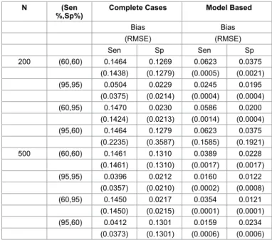
A simulation study was conducted to illustrate the reduction in bias and root mean squared error (RMSE) of the estimators for sensitivity and specificity for MAR model compared to complete case analysis (Table 4).
Two variables “Test Results” and “Disease Status” with different sample sizes (N) were generated from the multinomial distribution with marginal probabilities of πˆ = 0.5+1 and πˆ = 0.5+2 under different
sensitivity ( 11 1 =ππ + ) and specificity ( 22 2 =ππ + ) values. We cross-classified these variables in a 2 2× contingency table. This process was repeated
2000 times. In each complete contingency tables, we generated missing values in “Disease Status” in such a way that missingness in “Disease Status” depends on the realization of the “Test Results” to ensure the MAR missing mechanism. Table 4 represents the results from our simulation for MAR model when 50% of negative tests and 10% of the positive tests were not verified for the disease. Table 4 shows that correcting for the verification bias using the log-linear model approach will substantially reduce the bias as well as improve the performance
of the estimators compared to complete case analysis. We obtained similar results with 10% missigness in T+ with different amounts
of missingness in T− such as 70%, 60%, 40%, 30% and 20% and/or
various marginal probabilities. In addition to this, we carried out an extensive simulation for Model ( )β.j by simulating the MNAR missing
mechanism to estimate PPV and NPV. We observed the reduction in bias and RMSE compared to complete case analysis under different amounts of non-ignorable missingness on the disease status.
Application
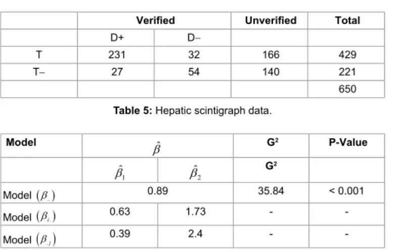
In this section, we will demonstrate the log-linear modeling approach to compute the measures of diagnostic accuracy under various missing mechanisms by using the Hepatic Scintigraph data published by [19]. In the Hepatic Scintigraph data, 650 patients underwent hepatic scintigraphy of which 429 patients had positive scans while 221 patients had negative hepatic scans. Only 263 patients out of 429 and 81 patients out of 221 were referred for status verification using procedures such as liver biopsy, exploratory laparotomy or autopsy within 6 weeks of their scans. Table 5 represents the verified and unverified cases by hepatic scan results. Table 6 shows the Maximum likelihood estimates for model parameters (Tables 5-7).
Table 7 represents the estimates of sensitivity, specificity , PPV and NPV and 95% confidence intervals under three different models by using the log-linear model approach to Table 5. By using Zhou [7] method the estimates of Sensitivity and Specificity can range from (0.68,0.95) and (0.37,0.86) respectively depending upon the values of
0
e and e1. From Table 7, it can be confirmed that under MAR and
MCAR assumptions the estimates of PPV and NPV and under MNAR assumption the estimates of sensitivity and specificity can be obtained from complete cases [8].
Final Remarks
Verification bias is an extremely common problem in diagnostic medicine. This paper shows that how the log-linear model approach in single binary-scale diagnostic tests correct the verification bias for estimating the diagnostic measures. Log-linear models also reduces
N (Sen
%,Sp%) Complete Cases Model Based
Bias Bias (RMSE) (RMSE) Sen Sp Sen Sp 200 (60,60) 0.1464 0.1269 0.0623 0.0375 (0.1438) (0.1279) (0.0005) (0.0021) (95,95) 0.0504 0.0229 0.0245 0.0195 (0.0375) (0.0214) (0.0004) (0.0004) (60,95) 0.1470 0.0230 0.0586 0.0200 (0.1424) (0.0213) (0.0014) (0.0004) (95,60) 0.1464 0.1279 0.0623 0.0375 (0.2235) (0.3587) (0.1585) (0.1921) 500 (60,60) 0.1461 0.1310 0.0389 0.0228 (0.1461) (0.1310) (0.0017) (0.0017) (95,95) 0.0396 0.0212 0.0160 0.0122 (0.0357) (0.0210) (0.0002) (0.0008) (60,95) 0.1450 0.0217 0.0354 0.0121 (0.1450) (0.0215) (0.0001) (0.0001) (95,60) 0.0412 0.1301 0.0159 0.0234 (0.0373) (0.1301) (0.0006) (0.0006) Table 4: Bias and MSE comparison for 50% missing in T − and 10% missing in T + .
the bias and improves the performance of the estimators compared to complete case analysis. In addition to this, explicit estimates for the measures of diagnostic accuracy under different missing mechanisms can be computed from simple algebraic formula, while other available methods require iterative methods to estimate the measures of diagnostic accuracy. Furthermore, this approach will allow us to test for MCAR assumption for particular data. However, the only way to confirm for MAR or MNAR missing mechanisms is to recollect the missing data. Although in diagnostic medicine due to the issue of cost-effectiveness, we do not have the luxury of getting hold of the missing data. As a result, careful modeling of missing mechanisms to reduce the bias is more an important issue. Therefore, if the data are not MCAR then by using the scientific knowledge about the data we can assume a MAR or MNAR missing mechanism to compute estimates for the measures of diagnostic accuracy with log-linear models.
Conflict of Interest
The authors have declared no conflict of interest.
References
1. Zweig MH, Campbell G (1993) Receiver-operating characteristic (ROC) plots: a fundamental evaluation tool in clinical medicine. Clin Chem 39: 561-577. 2. Nofuentes JAR, Castillo JDLD (2007) The effect of vericationbias in the nave
estimators of accuracy of a binary diagnostic test. Communications in Statistics: Simulation and Computation 36: 959-972.
3. Ransohoff DF, Feinstein AR (1978) Problems of spectrum and bias in evaluating
the efficacy of diagnostic tests. N Engl J Med 299: 926-930.
4. Begg CB, Greenes RA (1983) Assessment of diagnostic tests when disease
verification is subject to selection bias. Biometrics 39: 207-215.
5. Zhou XH (1998) Comparing accuracies of two screening tests in a two- phase study for dementia. Journal of the Royal Statistical Society: Series C (Applied Statistics) 47: 135-137.
6. Rubin DB (1976) Inference and missing data. Biometrika 63: 581-592. 7. Zhou XH (1993) Maximum likelihood estimators of sensitivity and specicity
corrected for veri_cation bias. Communications in Statistics - Theory and Methods 22: 3177-3198.
8. Zhou XH (1994) Effect of verification bias on positive and negative predictive
values. Stat Med 13: 1737-1745.
9. Harel O, Zhou XH (2006) Multiple imputation for correcting verification bias.
Stat Med 25: 3769-3786.
10. De Groot JA, Janssen KJ, Zwinderman AH, Bossuyt PM, Reitsma JB, et al.
(2011) Correcting for partial verification bias: a comparison of methods. Ann
Epidemiol 21: 139-148.
11.Baker SG (1995) Evaluating multiple diagnostic tests with partial verification.
Biometrics 51: 330-337.
12. Kosinski AS, Barnhart HX (2003) Accounting for nonignorable verification bias
in assessment of diagnostic tests. Biometrics 59: 163-171.
13. Martinez EZ, Achcar JA, Louzada-Neto F (2006) Estimators of sensitivity and specicity in the presence of verication bias: A bayesian approach. Computational Statistics and Data Analysis 51: 601-611.
14. Buzoianu M, Kadane JB (2008) Adjusting for verification bias in diagnostic test
evaluation: A Bayesian approach. Stat Med 27: 2453-2473.
15. Pepe M (2004) The Statistical Evaluation of Medical Tests for Classication and Prediction. Oxford University Press.
16. Zhou XN, Obuchowski, McClish D (2011) Statistical Methods in Diagnostic
Medicine. John Wiley and Sons Inc.
17. Baker SG1, Rosenberger WF, Dersimonian R (1992) Closed-form estimates
for missing counts in two-way contingency tables. Stat Med 11: 643-657. 18. Byrd RH, Lu P, Nocedal J, Zhu C (1995) A limited memory algorithm for bound
constrained optimization. SIAM Journal on Scientific Computing 16: 1190-1208.
19. Drum DE, Christacopoulos JS (1972) Hepatic scintigraphy in clinical decision making. J Nucl Med 13: 908-915.
Verified Unverified Total
D+ D−
T 231 32 166 429
T− 27 54 140 221
650 Table 5: Hepatic scintigraph data.
Model βˆ G2 P-Value 1 ˆ β βˆ2 G2 Model ( )β.. 0.89 35.84 < 0.001 Model ( )βi. 0.63 1.73 - - Model
( )
β.j 0.39 2.4 - -Table 6: ML estimates for model parameters.
Measure Model ( )β.. Model ( )βi. Model ( )β.j
Sensitivity 0.9 0.84 0.9 (0.86,0.93) (0.77,0.88) (0.85,0.93) Specificity 0.63 0.74 0.63 (0.52,0.73) (0.66,0.81) (0.52,0.72) PPV 0.88 0.88 0.75 (0.83,0.91) (0.84,0.91) (0.62,0.84) NPV 0.67 0.67 0.83 (0.55,0.77) (0.58,0.75) (0.75,0.89) Table 7: Estimates of diagnostic accuracy measures.
Appendix
Log-linear parameterization
Expected counts for all verified cases can be modeled by using equation 1 in the following way
11= exp{ ( ) ( ) (1) (1) ( ) ( 1) ( 1) ij I i J j RI RJ IJ ij IRI i IRJ i µ λ λ+ +λ +λ +λ +λ +λ +λ ( 1) ( 1) (11)} JRI j JRJ j R RI J λ λ λ + + +
Expected counts for all un-verified cases can be modeled as the following way :
12= exp{ ( ) ( ) (1) (2) ( ) ( 1) ( 2) ij I i J j RI RJ IJ ij IRI i IRJ i µ λ λ+ +λ +λ +λ +λ +λ +λ ( 1) ( 2) (12)} JR JR R R I j J j I J λ λ λ + + +
Some of the side conditions (the sum of each
λ-term over each of the indicated subscript is zero) for the log-linear
models are
2 2 2 2 =1 =1 =1 =1 ( ) = 0 ( ) = 0 ( ) = 0 (1 ) = 0 RJ JRJ IRJ R RI J k k k k k jk jk k λ λ λ λ∑
∑
∑
∑
By using these conditions, we can get
12 11 = ij = 2 exp{ (1) ( 1) ( 1) (11)} ij R IR JR R R J J J I J ij b µ λ λ i λ j λ µ − + + +Maximum likelihood (ML) Estimates for Model
( )
β..(MCAR)
( )
(
)
(
)
11 12 .. .. , , = ij log ij i log i ij 1 i j i i j L∑
n m +∑
n+ m+β −∑
m +β 12 , .. .. = i i ij i i i j n L m m m β +β + + ∂ ⋅ − ∂∑
∑
12 12 11 .. .. 11 .. ˆ ˆ ˆ 0 = However,forcompetedatam =n whichprovidestheMLestimatesfor = ˆ n n m n β β β ++ ++ ++ ++ ++ ++ ∴ − ∴( )
11 12(
)
ij .. ij .. .. .. MLestimatesform forModel canbederivedbytakingthederivativeofLwithrespecttom = ij i 1ij ij i n n L m m m β β β β + + ∂ ∴ + ⋅ − +
(
)
11 12 .. ˆ 0 = 1 ˆ ˆ ij i ij i n n m m β + + ∴ + − +(
)
11 12 .. ˆ 1 = ˆ ˆ ij i ij i n n m m β + + ∴ + + 12 12 .. 11 11 ˆ ˆ ˆ Substituting fromequation ?? 1 = ˆ i ij ij ij i n n m n m n m β ++ + ++ + ∴ + ⋅ + ⋅ 12 1 11 11 ˆ = ˆ ˆ i ij ij ij i n n m n m n m + ++ + ++ + ∴ ⋅ + ⋅ 12 11 11 1 ˆ = ˆ ˆ i ij ij ij i n n m n m m n + ++ + ++ + ∴ + ⋅ ⋅ (11)
First solving for
mˆi+12 11 11 1 ˆ = ˆ ˆ i i i i i n n m n m m n + ++ + + + + ++ + + ⋅ ⋅ 11 1 1 ˆi = i n m n n ++ + + + ++ + ∴ ⋅
Substituting
mˆi+in equation 11
11 1 11 1 11 ˆ = ij i ij i n n n m n n + + ++ ++ + + ⋅ ⋅ ⋅Maximum likelihood Estimates for Model
( )
βi.(MAR)
( )
(
)
(
)
11 12 . . , , = ij log ij i log i i ij 1 i i j i i j L∑
n m +∑
n+ m+β −∑
m +β 12 . . = i i ij j i i i n L m m m β +β + + ∂ ⋅ − ∂∑
(
)
11 12 . ˆ 0 = 1 ˆ ˆ ij i i ij i n n m m β + + ∴ + − +(
)
11 12 . ˆ 1 = ˆ ˆ ij i i ij i n n m m β + + ∴ + + 12 12 11 ˆ ˆ 1 = ˆ ˆ i i ij ij ij i i n n m n m m m + + + + ∴ + ⋅ + ⋅ (
mˆi+ ni+12)
mˆij=n mij11ˆi+ ni+12mˆij ∴ + ⋅ +(
12 12)
11 ˆij ˆi i i = ij ˆi m m+ n+ n+ n m+ ∴ ⋅ + − 11 ˆ =ij ij m n ∴Maximum likelihood Estimates for Model
( )
β.j(MNAR)
( )
(
)
11 12 . . , , = ij log ij i log ij j ij 1 j i j i j i j L n m n+ mβ m β + − + ∑
∑
∑
∑
12 . . = i ij ij i i j ij j j n L m m m β +β ∂ ⋅ − ∂ ∑
∑
∑
12 . ˆ ˆ 0 = ˆ ˆ i ij ij i ij j i j n m m mβ + ∴ ⋅ − ∑
∑
∑
( )
12 .j ij .j i 12 .j ij .j j . ˆ ˆ ˆ ˆˆ = ˆ Fromequation ??,wecanguessMLestimatesfor is m =n .MLestimatesform forModel canbederivedbytakingthederivativeofL ˆ ˆ i ij ij i i ij j j n m m mβ β β β β + + ∴ ⋅ ∀
∑
∑
∑
∑
(
)
11 12 . . . ˆ ˆ 0 = 1 ˆ ˆ ˆ ij i j j ij ij j j n n m mβ β β + ∴ + ⋅ − +∑
(
)
12 . 11 . . ˆ ˆ ˆ 1 = ˆ ˆ ˆ i ij j ij ij j ij j j n m n m m β β β + ∴ + + ⋅∑
(12)
( )
11 .j ˆ =ij ij WecaneasilycheckourguesssatiffyalltheMLequationforModel m n β ∴Comparison of MAR Estimates with Zhou’s Result
The [] estimates for Sensitivity is
(
1 1 1111)
1 1111 1211 1 1 1111 2 1 2111 1 1111 1211 1 2111 2211 ( ) ( ) = ( ) ( ) n n n n n Sensitivity Zhou n n n n n n n n n n + + ++ + + + + + ++ + ++ + + + + +(
1 1 1111)
2 11 1 1 1111 2 11 2 1 2111 1 11 = n n n n n n n n n + + + + + + + + + +(13)
From equation 6 the Sensitivity estimates from log-linear model are
(
)
(
)
(
11)
1.(
)
11 1. 21 2. ˆ ˆ 1 = ˆ ˆ ˆ 1 ˆ 1 m Sensitivity MAR m m β β β + + + +1 12 1111 1 1 12 2 12 1111 2111 1 2 1 ˆ = 1 1 ˆ ˆ n n m n n n n m m + + + + + + + + + + 1 12 1111 1 11 1 12 2 12 1111 2111 1 11 2 11 1 = 1 1 n n n n n n n n n + + + + + + + + + +
(
1 1 1111)
2 11 1 1 1111 2 11 2 1 2111 1 11 = n n n =Sensitivity Zhou( ) n n n n n n + + + + + + + + + +Similarly, we can show that the estimates for Specificity from log-linear models are equivalent to [] Specificity
estimates.
Information Matrices :
Model
( )
β.. 2 12 2 2 .. .. = n L β β++ ∂ − ∂ 2 .. 12 2 2 2 .. .. .. .. = n =m =m L E E β β β++ β++ β++ ∂ − ∂ 2 .. 1 = ij ij i L E m m m β + ∂ − + ∂ 2 .. = 1 ij L E mβ ∂ − ∂ 2 2 2 2 2 2 11 11 12 11 21 11 22 11 .. 2 2 2 2 2 2 12 11 12 12 21 12 22 12 .. 2 21 11 = L L L L L E E E E E m m m m m m m m L L L L L E E E E E m m m m m m m m L E E m m β β ∂ ∂ ∂ ∂ ∂ − ∂ − ∂ − ∂ − ∂ − ∂ ∂ ∂ ∂ ∂ ∂ − ∂ − ∂ − ∂ − ∂ − ∂ ∂ ∂ − ∂ − 1 I 2 2 2 2 2 21 12 21 21 22 21 .. 2 2 2 2 2 2 22 11 22 12 22 21 22 22 .. 2 2 2 .. 11 .. 12 .. L L L L E E E m m m m m m L L L L L E E E E E m m m m m m m m L L L E E E m m β β β β β − ∂ − ∂ − ∂ ∂ ∂ ∂ ∂ ∂ ∂ ∂ ∂ ∂ − ∂ − ∂ − ∂ − ∂ − ∂ ∂ ∂ ∂ − ∂ − ∂ − ∂ 2 2 2 21 .. 22 .. L L E E m βm β − ∂ − ∂ ∂ ∂ Model
( )
βi. 2 2 . . = i i i m L E β β+ ∂ − ∂ 2 . 1 = i ij ij i L E m m m β + ∂ − + ∂ 2 . = 1 ij i L E mβ ∂ − ∂ = 2 I 2 21 11 21 12 21 21 22 21 1. 21 2. 2 2 2 2 2 2 22 11 22 12 22 21 22 22 m m m m m m m m m L L L L L E E E E E m m m m m m m m β β ∂ ∂ ∂ ∂ ∂ ∂ ∂ ∂ ∂ ∂ ∂ − − − − − ∂ ∂ ∂ ∂ ∂ 2 1. 22 2. 2 2 2 2 2 2 2 1. 11 1. 12 1. 21 1. 22 1. 1. 2. 2 2 2 2 2. 11 2. 12 2. 21 2. 22 L E m L L L L L L E E E E E E m m m m L L L L E E E E m m m m β β β β β β β β β β β β β − ∂ ∂ ∂ ∂ ∂ ∂ ∂ ∂ − ∂ − ∂ − ∂ − ∂ − ∂ − ∂ ∂ ∂ ∂ ∂ − ∂ − ∂ − ∂ − ∂ 2 2 2 2. 1. 2. L L E E β β β ∂ ∂ − − ∂ ∂
Model
( )
β.j( )
(
)
2 2 2 . . = ij i j ij j j m L E m β β ∂ − ∂ ∑ ∑
( )
(
)
2 2 . . 1 = j ij ij ij j j L E m m m β β ∂ − + ∂ ∑
(
)
2 . . . = ij j ij i ij j j m L E m m β β β ∂ − ∂ ∑
2 2 2 2 2 2 2 11 11 12 11 21 11 22 11 .1 11 .2 2 2 2 2 2 2 12 11 12 12 21 12 22 12 .1 = L L L L L L E E E E E E m m m m m m m m m L L L L L E E E E E E m m m m m m m m β β β ∂ ∂ ∂ ∂ ∂ ∂ − ∂ − ∂ − ∂ − ∂ − ∂ − ∂ ∂ ∂ ∂ ∂ ∂ ∂ − ∂ − ∂ − ∂ − ∂ − ∂ − 3 I 2 12 .2 2 2 2 2 2 2 2 21 11 21 12 21 21 22 21 .1 21 .2 2 2 2 2 2 2 22 11 22 12 22 21 22 22 L m L L L L L L E E E E E E m m m m m m m m m L L L L L E E E E E m m m m m m m m β β β ∂ ∂ ∂ ∂ ∂ ∂ ∂ − − − − − − ∂ ∂ ∂ ∂ ∂ ∂ ∂ ∂ ∂ ∂ ∂ − ∂ − ∂ − ∂ − ∂ − ∂ 2 .1 22 .2 2 2 2 2 2 2 2 .1 11 .1 12 .1 21 .1 22 .1 .1 .2 2 2 2 2 .2 11 .2 12 .2 21 .2 22 L E m L L L L L L E E E E E E m m m m L L L L E E E E m m m m β β β β β β β β β β β β β − ∂ ∂ ∂ ∂ ∂ ∂ ∂ ∂ − ∂ − ∂ − ∂ − ∂ − ∂ − ∂ ∂ ∂ ∂ ∂ − ∂ − ∂ − ∂ − ∂ 2 2 2 .2 .1 .2 L L E E β β β ∂ ∂ − ∂ − ∂ Likelihood Ratio Statistics
Model
( )
β..11
2 12 12
11 12 12
, .. ..
= 2 log log log
ˆ ˆ ˆ ˆ ˆ ij i ij i i j ij i i n n n G n n n m m β m β + ++ + ++ + ++ + +
∑
∑
( )
2 11 12(
12)
i. 11 12 12 , . .Model = 2 log log log
ˆ ˆ ˆ ˆ ˆ ij i ij i i j ij i i i i i i n n n G n n n m m m β β β + ++ + ++ + + + +
∑
∑
∑
( )
2 11 12(
12)
.j 11 12 12 , . .Model = 2 log log log
ˆ ˆ ˆ ˆ ˆ ij i ij i i j ij i ij j j j j j n n n G n n n m m m β β β + ++ + ++ + + +
∑
∑
∑
∑