Calhoun: The NPS Institutional Archive
Faculty and Researcher Publications Faculty and Researcher Publications
2014-01
A Bayesian beta kernel model for binary
classification and online learning problems
MacKenzie, Cameron A.
Preprint submitted to Statistical Analysis and Data Mining January 21, 2014
http://hdl.handle.net/10945/39499
A Bayesian beta kernel model for binary classification
and online learning problems
Cameron A. MacKenziea, Theodore B. Trafalisb, Kash Barkerb This is an author’s manuscript that has been submitted for publication in the journal
Statistical Analysis and Data Mining. (January 21, 2014)
aDefense Resources Management Institute, Naval Postgraduate School, Monterey, CA 93943 bSchool of Industrial and Systems Engineering, University of Oklahoma, Norman, OK
73019
Abstract
Recent advances in data mining have integrated kernel functions with Bayesian probabilistic analysis of Gaussian distributions. These machine learning ap-proaches can incorporate prior information with new data to calculate proba-bilistic rather than deterministic values for unknown parameters. This paper extensively analyzes a specific Bayesian kernel model that uses a kernel function to calculate a posterior beta distribution that is conjugate to the prior beta dis-tribution. Numerical testing of the beta kernel model on several benchmark data sets reveals that this model’s accuracy is comparable with those of the support vector machine, relevance vector machine, naive Bayes, and logistic regression, and the model runs more quickly than other algorithms. When one class oc-curs much more frequently than the other class, the beta kernel model often outperforms other strategies to handle imbalanced data sets, including under-sampling, over-under-sampling, and the Synthetic Minority Over-Sampling Technique. If data arrive sequentially over time, the beta kernel model easily and quickly updates the probability distribution, and this model is more accurate than an incremental support vector machine algorithm for online learning.
1. Introduction
Since advances in the mid-1990s, kernel-based approaches to machine learn-ing and pattern recognition have revolutionized the field of data minlearn-ing (Shawe-Taylor and Cristianini 2004). Kernel functions map input data to a higher di-mensional space, called the feature space, where the dot product between two vectors in the feature space is replaced by a kernel function. This approach enables algorithms designed to detect linear relationships in data, such as sup-port vector machines (SVM) and least-squares regression, to detect non-linear relationships and patterns through their use on the feature space (Cristianini and Shawe-Taylor 2000; Hastie et al. 2001; Sch¨olkopf and Smola 2002).
More recently, kernel functions have been integrated with Bayesian analysis to produce a new subset of machine learning tools that produce probabilistic rather than deterministic solutions. Probabilistic outcomes can better express uncertainty in underlying data relative to deterministic outcomes. Most pre-vious Bayesian kernel models, such as the relevance vector machine (RVM), have assumed Gaussian prior distributions over model parameters (Seeger 2000; Tipping 2001; Sch¨olkopf and Smola 2002; Bishop and Tipping 2003). Different approaches, such as assuming the mean and variance of the Gaussian distri-bution are randomly chosen from other distridistri-butions, have been deployed to increase the flexibility and accuracy of the Gaussian kernel model (Figueiredo 2002; Mallick et al. 2005; Zhang et al. 2011). These approaches carry additional computational complexities and generally require simulation algorithms such as Markov Chain Monte Carlo to solve for the optimal parameters.
At least two issues can pose challenges to kernel-based binary classifiers, including the Gaussian Bayesian models. First, imbalanced data sets, where one class appears much more frequently than another class, create difficulties for many machine learning algorithms because the classifiers tend to classify almost all of the unknown data points in the class that occurs most frequently. Second, most classifiers are designed to process data in a single batch, and a classifier may have difficulty in incrementally updating if data arrive sequentially. Although
Bayesian models can typically use new information to update a probability distribution, the complexity of Gaussian kernel models limits their ability to update quickly.
A Bayesian kernel model using the beta rather than the normal distribu-tion can potentially address both of these challenges. The beta kernel model appears to have been first presented by Montesano and Lopes (2009) in order to predict a robot’s ability to grasp objects. The authors used empirical proba-bilities calculated from previous experiments with the robot to update the beta distribution. Although the beta kernel model was developed specifically for this robotic application, we believe the model deserves a fuller exploration. This paper analyzes the beta kernel model for a wider range of binary classification problems where empirical probabilities are unavailable, the data are heavily im-balanced, and data arrive incrementally. Additionally, the beta kernel model does not require solutions to optimization problems such as the SVM or RVM, which makes the beta kernel model extremely fast to calculate.
This paper offers several unique contributions to analyze whether beta kernel models should become part of the machine learning toolkit for binary classifica-tion problems. We explicitly relate the beta kernel model to the beta-binomial Bayesian model and discuss how to select parameters for the prior distribution. We generalize the beta kernel model to a Dirichlet kernel model that could be used for multiclass classification problems. This paper also explores the similar-ities of the beta kernel and the well-known Parzen (1962) window classifier and discusses how the beta kernel model can overcome some of the difficulties with the Parzen window. Our inclusion of weighting parameters with the likelihood function in the beta kernel model or beginning with a non-uniform prior distri-bution increases the predictive accuracy for imbalanced data sets. Finally, the posterior probabilities from the model can act as prior probabilities to incorpo-rate additional information, making the model useful for online or incremental learning.
Section 2 focuses on binary classification problems. We review the existing Gaussian kernel models such as the RVM and the beta kernel model presented
by Montesano and Lopes (2009). The model can be extended to imbalanced data sets through the addition of weighting parameters or a non-uniform prior. Section 3 extensively tests the beta kernel model, the RVM, and the SVM for standard binary classification problems, heavily imbalanced data sets, and online learning. Tests on imbalanced data sets include additional algorithms such as under-sampling and over-sampling in combination with the RVM and SVM.
2. Bayesian models
Binary classification machine learning tools seek to assign an unknown data point y either to the negative class, y = −1, or to the positive class, y = 1. The assignment is based on the input data x, a vector with d components, where each component is an attribute. Rather than assigning y to either the positive or negative class, Bayesian binary classification models calculate the probability thaty belongs to each class givenx. Because most Bayesian kernel models assume Gaussian prior distributions, we first present the basic Gaussian kernel model and the popular RVM (a variation of the basic model) and next the beta kernel model.
2.1. Gaussian kernel model
Gaussian Bayesian kernel models assume a functiont maps the input data xto a target value that corresponds to an outputy, wherey∈ {−1,+1}. The range oft(x) is the set of all real numbers, and the logit function mapst(x) to a probability thaty= 1.
P(y= 1|t(x)) = 1
1 + exp(−t(x)) (1)
If them×ddata matrixXhasmrows (observed data points) each withd attributes, the functiont(X) can be thought of as a random vector of lengthm. The Gaussian model assumes thattfollows a multivariate normal distribution where E[t] =0and Cov(t) =K (Sch¨olkopf and Smola 2002). The matrix Kis
positive definite whereKij is the kernel function k(xi,xj) between theith and jth data points. P(t) = p 1 (2π)m(detK) −1/2exp −1 2t TK−1t (2)
Calculating the inverse of K is computationally expensive, and a new vector
ω of length m is introduced such that t(xi) = P m
j=1k(xi,xj)ωj = k(xi,X)ω
(Sch¨olkopf and Smola 2002). The prior probability function for ω is also a multivariate normal distribution but eliminates the need to take the inverse of K. P(ω) =p 1 (2π)m(detK) −1/2exp −1 2ω TKω (3) Because √ 1 (2π)m(detK)
−1/2 does not depend on ω, the prior can be written without this constant. With the likelihood from (1) and the prior from (3), the posterior becomes a function ofωand the observed output valuesy.
P(ω|y) = m Y i=1 1 1 + exp(−k(xi,X)ω) 0.5+0.5yi 1 1 + exp(k(xi,X)ω) 0.5−0.5yi exp −1 2ω TKω (4) Most solution methods seek to maximize the posterior or equivalently, to mini-mize the negative of the log of the posterior (Sch¨olkopf and Smola, 2002). The Newton-Raphson method can be used to find ω that maximizes the posterior probability in (4). The posterior probability is identical to the objective function in non-Bayesian kernel logistic regression, which can be solved quickly using a truncated Newton method (Maalouf and Trafalis 2008).
An alternative to the logit link function in (1) is the probit model, which generally assumes that the sign of t(x) determines the class of y, except for Gaussian noise. If y= sgn (t(x+ξ) whereξ∼ N(0, σ), thenP(y= 1|t(x)) = Φ (yt(x)/σ) where Φ (·) is the standard normal cumulative distribution (Sch¨olkopf
and Smola 2002). Figueiredo (2002) uses the probit model to build a hierarchi-cal Bayesian kernel model where most of the weights—which play a role similar toωin (3)—are 0.
2.2. Relevance vector machine
Although several variations on the Gaussian Bayesian kernel model exist (e.g., Figueiredo 2002; Mallick et al. 2005; Zhang et al. 2011), the most pop-ular extension of this model is perhaps the RVM. The RVM seeks to combine the sparsity aspects of the SVM with the probabilistic advantages of Bayesian methods (Tipping 2001; Bishop and Tipping 2003). The SVM assigns non-zero weights to only a small fraction of the total number of data points, and the RVM seeks to find a similarly sparse set.
The RVM has the same logit likelihood function as in (1); however, the prior onωbecomes a function of a hyperparameters, where eachsj is the inverse of
the variance ofωj (Tipping 2001). The conditional probability density function
ofωgivensis expressed in (5) whereS=diag(s) (Bishop and Tipping 2003). P(ω|s) =p 1 (2π)m(detS) 1/2 exp −1 2ω TSω (5) Traditionally, eachsj ≥0 is assumed to be drawn from the same gamma
distri-bution as given in (6) where Γ(·) is the gamma function.
P(sj) = ba Γ(a)s a−1 j e −bsj (6)
The shape and scale parameters,aand b, respectively, are usually set close to 0 to ensure a flat or non-informative prior over ω. If a → 0 and b → 0, the gamma distribution becomes degenerate such that si = 0 in the limit, which
implies infinite variance forωi (Sch¨olkopf and Smola 2002).
The RVM algorithm (Tipping and Faul 2003) begins by selecting the data point that maximizes the posterior probability, and it sequentially adds addi-tional data points until the posterior probability begins to converge to a value. Because E[ωi] = 0, only a few ωi’s are non-zero. Testing the RVM on
sev-eral databases reveals that approximately 10% of theωi’s are non-zero and the
RVM’s error rate is comparable to that of the SVM (Tipping 2001; Bishop and Tipping 2003). The RVM has been applied to a wide variety of problems such as analyzing remote sensor data (Foody 2008), forecasting stock indices (Huang and Wu 2008), and estimating battery reliability (Saha et al. 2009).
The Gaussian distribution enables analytically tractable solutions, and the RVM delivers sparse solutions. As justification for a normal distribution over the prior, each target valuetiis a linear-weighted sum of a multivariate random
vector ω where ω∼ N(0,K−1) for the basic Gaussian kernel model and ω∼ N(0,S−1) in the RVM. Thus, eacht
i also follows a normal distribution.
2.3. Beta kernel model
Alternatively, the beta distribution can serve as a prior distribution for Bayesian models. The beta distribution is a natural model for binary out-comes because the distribution’s two parameters can represent the number of times each outcome has occurred or is expected to occur (Gupta and Nadarajah 2004), and the distribution provides the probability distribution of a parameter θ∈[0,1] where θ=P(y = 1) and 1−θ=P(y =−1). We begin the develop-ment of the beta distribution as a prior distribution for classification problems by examining the model as applied to predict a robot’s ability to grasp objects. Generalizing this model and adding weighting parameters enables us to apply this model to a broad spectrum of binary classification problems.
The beta distribution can model a Bernoulli process whereαis the number of successes and β is the number of failures. If the prior on θ follows a beta distribution with prior parameters α and β and the Bernoulli process results inrsuccesses out ofmtrials, which implies a binomial likelihood function, the posterior distribution overθalso follows a beta distribution.
θ|r∼beta(α+r, β+m−r) (7)
The beta distribution is known as a conjugate prior because the posterior is also a beta distribution.
Montesano and Lopes (2009) and Mason and Lopes (2011) exploit the beta-binomial relationship by adapting it to a data mining problem that slightly differs from the binary classification problem we have been discussing. In their problem, eachxj hasNj trials, withRj positive classifications andUj negative
classifications, where Rj +Uj = Nj. An empirical probability of a positive
classificationyj = 1 exists for each data point, ˆθj= Rj/Nj.
For a data pointxi whose empirical probability is unobserved or unknown,
the kernel function,k(xi,xj), serves as a measure of similarity betweenxi and
xj. In this manner, the kernel function can be used to estimate the posterior
distribution forθi based on the observedRj andUj formdata points.
θi|Rj, Uj∼beta α+ m X j=1 k(xi,xj)Rj, β+ m X j=1 k(xi,xj)Uj (8)
The most likely estimate ¯θi= E [P(yi= 1)] is the expected value of the beta
posterior distribution. ¯ θi= α+Pm j=1k(xi,xj)Rj α+Pm j=1k(xi,xj)Rj+β+P m j=1k(xi,xj)Uj (9) An optimization algorithm selects parameters for the kernel function by minimizing the squared difference between the ¯θj as calculated by (9) and the
empirical probability ˆθj for a training set (Montesano and Lopes, 2009). This
Bayesian kernel regression allows the authors to measure a robot’s ability to grasp different objects (which have a set of features) and then use those results to estimate the probability that a robot will grasp a different object that has not been empirically measured.
Empirical probabilities are generally not available for binary classification problems because each data pointxjoften has a single trial rather than multiple
trials, i.e.,Nj = 1 for allj= 1, . . . , m. Another potential problem that plagues
many binary classifiers is inaccurate classifications if the two classes do not contain the same number of data points (King and Zheng 2001; Wang et al. 2010; Maalouf and Trafalis 2011). Many machine learning tools label too many
points in the class that occurs most frequently. We resolve this problem of imbalanced data sets by including weighting parameters m−/m and m+/m, wherem−andm+ are the number of negative and positive labels, respectively, in the training set.
θi|y∼beta α+ m− m X {j|yj=1} k(xi,xj), β+ m+ m X {j|yj=−1} k(xi,xj) (10)
These weighting parameters balance the likelihood function so that the posterior probability moves to whichever class is closest toxiin the feature space. These
parameters follow typical cost penalties or weights for the SVM (Morik et al. 1999; Wang and Japkowicz 2008). In a weighted SVM, the ratio of misclassifi-cation in the positive class to misclassifimisclassifi-cation in the negative class weight often is m−/m+.
As a Bayesian formulation, (10) calculates a probability distribution over θi=P(yi = 1) based on a set of known data points. The parameters of the beta
distribution are updated for θi so that αi =α+ (m−/m)P{j|yj=1}k(xi,xj)
andβi=β+(m+/m)P{j|yj=−1}k(xi,xj). The expected value of the posterior
distribution ¯θi= αi/(αi+βi) can be used for making predictions.
This beta kernel model can be generalized to multiclass classification prob-lems by deploying a Dirichlet distribution. The Dirichlet distribution describes the probability ofN discrete outcomes. Given a Dirichlet prior with prior pa-rametersα1, α2, . . . , αN, the weighted kernel approach in (11) derives the
pos-terior probability forθi, which also follows a Dirichlet distribution. The weight
to update αn is given by m−n/m, the fraction of points not in the nth class
whered= 1,2, . . . , N. θi|y∼Dir α1+ m−1 m X {j|yj=1} k(xi,xj), . . . , αN+ m−D m X {j|yj=N} k(xi,xj) (11)
The expected probability that an unknown data pointyi belongs to thenth
class is given by E [θi,n] =αi,n/αi,0 whereαi,n=αn+(m−n/m)P{j|yj=n}k(xi,xj)
andαi,0 =P
N
l=1αi,l. The posterior marginal distribution for each θi,n follows
a beta distribution whereθi,n ∼beta (αi,n, αi,0−αi,n).
This paper focuses on the specific case of the beta distribution and binary classification problems and examines numerical results for the beta kernel model. Future research can test the more general Dirichlet kernel model for multiclass classification problems.
We have previously been assuming that the prior αand β are given, and neither Montesano and Lopes (2009) nor Mason and Lopes (2011) devote much discussion to selecting prior distributions. If nothing is knowna prioriabout the probability of a positive or negative class, choosing a uniform prior whereα= 1 andβ = 1 may be the best. However, many situations arise where the overall probability of an event may be estimated based on past experience or data. For example, if the data mining problem is to predict breast cancer in women age 40 to 49, we might know that a randomly selected female in her 40s has a 2 percent chance of being diagnosed with breast cancer. The prior distribution can reflect that knowledge through the prior mean α/(α+β) = 0.02.
Data from the training set can be used to generate a prior distribution. The parametersαand β can be selected so that the mean equals the fraction of positively classified data points in the training set m+/m and so that the variance of the prior αβ.h(α+β)2(α+β+ 1)i matches the variance in the training set. An empirical Bayes method estimatesαandβ by maximizing the log-likelihood of the beta distribution. The Jeffreys prior where α= 0.5 and β = 0.5 has modes at the two ends of the distribution 0 and 1, but if a large number of data points exist in the training set (e.g., m > 20), the posterior distribution from a Jeffreys prior will closely resemble the posterior from a uniform prior. (Carlin and Louis 2008 present a helpful discussion on selecting priors for Bayesian analysis.)
The prior may also influence if the weighting parameters,m−/mand m+/m, are used. Probabilistic data mining models often include a threshold probability
that divides the positive and negative classes. With a uniform prior, if the ex-pected value of the posterior distribution is greater than 0.5, the unknown point should be positively classified. The weighting parameters help ensure that this classification is due to the unknown data point’s similarity with the known data as opposed to one class being more numerous than the other class. Including weights is not appropriate with a non-uniform prior distribution, however, be-cause the weights would generate a posterior whose expectation is too close to the class with fewer data points. If a non-uniform prior is used, no weighting parameters are necessary. Instead, the expectation of the prior distribution can be used as the threshold probability so that if the expectation of the poste-rior is greater than the expectation of the pposte-rior, the point should be positively classified. Choosing between a uniform prior with weighting parameters and a non-uniform prior without weighting parameters can result in the same classifi-cation scheme, as the follow proposition illustrates.
Proposition 1. The following classification rules are equivalent.
1. Given a uniform prior whereα= 1andβ = 1and the weights as depicted in (10), an unknown pointyi should be positively classified ifθ¯i>0.5 and
negatively classified ifθ¯i<0.5.
2. Given a non-uniform prior where α/(α+β) = m+/m and if weights
are not deployed to update θi, an unknown point yi should be positively
classified ifθ¯i> m+/m and negatively classified ifθ¯i< m+/m.
Proof. See Appendix.
Although a uniform prior and weights will generate different posterior proba-bilities than a non-uniform prior without weights, the final classification schemes will be the same if the expected value of the non-uniform prior equals m+/m.
The beta kernel model closely resembles the Parzen (1962) window classifier, which classifies an unknown data point based on whether it is closer in the fea-ture space to the mean of the positive or negative class. An unknown data point yiis positively classified ifP{j|yj=1}k(xi,xj)
.
m+ > P{j|yj=−1}k(xi,xj)
.
An alternative interpretation of the Parzen window is that the unknown data point is labeled according to whether the probability is greater for the positive or negative class (Chapelle 2005). The probability thatyiis in the positive class
is P
{j|yj=1}k(xi,xj)
. Pm
j=1k(xi,xj) . The Parzen window probability echoes
the expectation of an unweighted posterior beta distribution.
A problem with using the Parzen window probability and the expectation of the beta posterior distribution occurs when a pointxiis far away in the feature
space from both positively and negatively classified points. If the point is slightly closer to the positive class, the Parzen window and the expectation of the beta distribution will likely calculate a high probability thatyi= 1 (Chapelle 2005).
In the Bayesian model, the posterior’s variance can express uncertainty in the classifier. Ifxi is dissimilar to the known points, bothP{j|yj=1}k(xi,xj) and
P
{j|yj=−1}k(xi,xj) should be close to zero, which implies the variance of the
posterior distribution P(yi|y) will be large, assuming α and β are relatively
small. Although the posterior distribution’s expectation may be high, the large variance would indicate a significant likelihood that the unknown point should be negatively classified.
3. Numerical results
3.1. Binary classification for the beta kernel, RVM, and SVM
We test the beta kernel model on several data sets and compare the results to the RVM, the traditional soft-margin SVM (Cristianini and Shawe-Taylor 2000; Shawe-Taylor and Cristianini 2004), a weighted soft-margin SVM (Chew et al. 2001), the naive Bayes algorithm, and logistic regression. The SVM is a kernel-based linear classifier that uses a relatively small number of vectors to create a boundary between the classes in the feature space. The soft-margin SVM assigns a cost parameter for misclassifications. In the weighted SVM, we assign a different cost for the misclassification of each class: Cm−/m for the positive
class andCm+/m for the negative class whereCis a constant cost parameter to be optimized. We use LIBSVM 3.0 (Chang and Ling 2001) for the SVM models
and the code developed by Tipping (2009) for the RVM. The classification rule for the beta kernel model follows Proposition 1. Matlab (2012) provides a naive Bayes classification algorithm that uses a kernel smoothing density estimate based on a normal distribution. The logistic regression algorithm is a non-kernel generalized linear regression model with a logit link function that positively labels an unknown data point if the calculated probability exceeds the fraction of positively classified data points in the training set.
Table 1 shows characteristics of the ten data sets used for comparing among the different classifiers. The Parkinson data set contains biomedical voice mea-surements that correspond to individuals with Parkinson’s disease and those without the disease (Little et al. 2009). Haberman’s survival database con-sists of patients who survived or died after undergoing surgery for breast cancer (Haberman 1976). The satellite data set contains spectral values for pixels in or-der to classify land images as red or gray soil. The arcene data contain patients with ovarian or prostrate cancer and healthy patients, where the attributes are mass-spectrometry features (Guyon et al. 2004). The spam database is a collec-tion of emails classified as either spam or not spam, and the attributes consist of frequency counts of words and characters. The adult data consist of census information from the U.S. 1994 census to predict whether or not an individual earns more or less than $50,000 (Kohavi 1996). The transfusion data set con-tains blood donor attributes to predict whether or not an individual donated blood in a specific month (Yeh et al. 2008). The breast cancer data use im-age characteristics of breast mass to predict if women will have a recurrence of breast cancer within two years of treatment (Street et al. 1995). These eight data sets can be downloaded from the University of California-Irvine Machine Learning Repository (Bache and Lichman 2013). The colon cancer data consists of gene expressions that either come from a tumor biopsy or a healthy biopsy, and this data derives from the Princeton University Gene Expression Project (Alon et al., 1999). Finally, the tornado database contains weather character-istics corresponding to a tornado or no tornado as collected by the National Weather Center at the University of Oklahoma (Trafalis et al. 2007).
Table 1: Binary classification data sets Data set Percentage of Number of attributes Training set size Tuning set size Testing set size positively labeled points Parkinson 75 22 98 39 58 Haberman’s survival 74 3 153 61 92 Satellite 53 36 509 203 305 Arcene 44 9,961 100 40 60 Spam 39 57 230 92 138 Colon cancer 35 2,000 31 12 19 Adult 24 13 799 320 480 Transfusion 24 4 374 150 224 Breast cancer 20 32 69 28 41 Tornado 7 83 541 216 325
With one exception, the radial basis function (RBF) is used as the kernel function throughout this paper, whereσ >0 is tuned to optimize each classifier.
k(xi,xj) = exp −||xi−xj|| 2 2σ2 (12) The RBF is perhaps the most popular kernel function because the image of the function lies between zero and one and the kernel matrix has full rank (Sch¨olkopf and Smola 2002).
The polynomial kernel has performed well in classifying text and spam data (Kudo and Matsumoto 2003; Moon et al. 2004). In addition to the RBF, we use the polynomial kernel on the spam data set for the beta kernel, RVM, and SVM algorithms. The polynomial kernel has two parameters: the degree of the polynomial functionp >0 and a constant parameterκ >0.
k(xi,xj) = (x|ixj+κ) p
(13) Each of the ten data sets is divided into a training, tuning, and testing set. The training set comprises 50 percent of each data set, the tuning set 20 percent, and the testing set 30 percent. In each individual trial,σin the RBF orpandκ in the polynomial kernel (as well as the cost parameterCin the SVM) is selected
that achieves the highest accuracy score in the tuning set. (The accuracy score is described in the next paragraph.) The training and tuning set are combined to retrain the classifier using the optimalσ orp andκ(and C) and test it on the testing set.
We repeat this procedure 200 times for each classifier, randomly selecting the training, tuning, and testing set for each trial. Table 2 displays the mean performance for the true positive (TP) rate, the true negative (TN) rate, and the accuracy score where Acc = √TP∗TN is the geometric mean (Kubat et al. 1997). The geometric mean explicitly penalizes a classifying algorithm that performs badly in classifying one of the classes. The receiver operating characteristic (ROC) curve can judge the performance of probabilistic classifiers such as the beta kernel and RVM and can be extended to include deterministic classifiers such as the SVM. We also calculate the area under the ROC curve (AUC) for each of the six classifiers for each of the 200 runs.
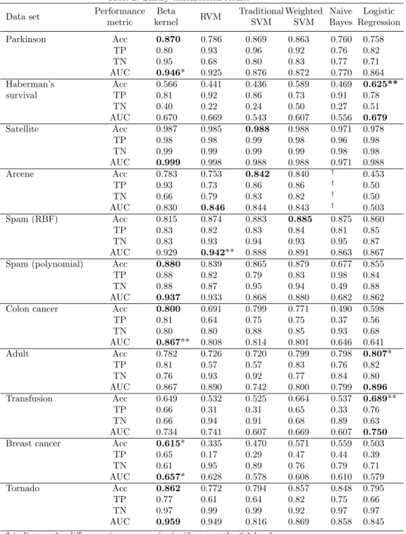
The results show that the beta kernel model performs comparably to the other data mining algorithms for these ten data sets. The beta kernel model has the highest average accuracy for five of the eleven data trials. (The spam data set is tested twice, once with the RBF kernel and once with the polynomial kernel.) Because we are making multiple comparisons of mean accuracy levels where the sample sizes are equal (200 repetitions), we use Tukey’s method to assess the statistical significance of the difference between the best performing classifier and the other classifiers. The beta kernel model’s mean accuracy is significantly different at the 0.1 level for the breast cancer data set. Logistic regression has the highest average accuracy for three data sets (Haberman’s survival, adult, and transfusion) and the difference in accuracy is significant at the 0.01 level for two data sets. However, logistic regression performs quite badly for the arcene and breast cancer data. The traditional SVM has the highest average accuracy for the satellite and arcene data, and the weighted SVM has the highest average accuracy for spam with the RBF kernel.
The beta kernel model performs quite well according to the AUC metric. The beta kernel has the largest average AUC for six data sets (Parkinson, satellite,
Table 2: Binary classification results
Data set Performance Beta RVM Traditional Weighted Naive Logistic
metric kernel SVM SVM Bayes Regression
Parkinson Acc 0.870 0.786 0.869 0.863 0.760 0.758 TP 0.80 0.93 0.96 0.92 0.76 0.82 TN 0.95 0.68 0.80 0.83 0.77 0.71 AUC 0.946* 0.925 0.876 0.872 0.770 0.864 Haberman’s Acc 0.566 0.441 0.436 0.589 0.469 0.625** survival TP 0.81 0.92 0.86 0.73 0.91 0.78 TN 0.40 0.22 0.24 0.50 0.27 0.51 AUC 0.670 0.669 0.543 0.607 0.556 0.679 Satellite Acc 0.987 0.985 0.988 0.988 0.971 0.978 TP 0.98 0.98 0.99 0.98 0.96 0.98 TN 0.99 0.99 0.99 0.99 0.98 0.98 AUC 0.999 0.998 0.988 0.988 0.971 0.988 Arcene Acc 0.783 0.753 0.842 0.840 † 0.453 TP 0.93 0.73 0.86 0.86 † 0.50 TN 0.66 0.79 0.83 0.82 † 0.50 AUC 0.830 0.846 0.844 0.843 † 0.503 Spam (RBF) Acc 0.815 0.874 0.883 0.885 0.875 0.860 TP 0.83 0.82 0.83 0.84 0.81 0.85 TN 0.83 0.93 0.94 0.93 0.95 0.87 AUC 0.929 0.942** 0.888 0.891 0.863 0.867
Spam (polynomial) Acc 0.880 0.839 0.865 0.879 0.677 0.855
TP 0.88 0.82 0.79 0.83 0.98 0.84
TN 0.88 0.87 0.95 0.94 0.49 0.88
AUC 0.937 0.933 0.868 0.880 0.682 0.862
Colon cancer Acc 0.800 0.691 0.799 0.771 0.490 0.598
TP 0.81 0.64 0.75 0.75 0.37 0.56 TN 0.80 0.80 0.88 0.85 0.93 0.68 AUC 0.867** 0.808 0.814 0.801 0.646 0.641 Adult Acc 0.782 0.726 0.720 0.799 0.798 0.807* TP 0.81 0.57 0.57 0.83 0.76 0.82 TN 0.76 0.93 0.92 0.77 0.84 0.80 AUC 0.867 0.890 0.742 0.800 0.799 0.896 Transfusion Acc 0.649 0.532 0.525 0.664 0.537 0.689** TP 0.66 0.31 0.31 0.65 0.33 0.76 TN 0.66 0.94 0.91 0.68 0.89 0.63 AUC 0.734 0.741 0.607 0.669 0.607 0.750
Breast cancer Acc 0.615* 0.335 0.470 0.571 0.559 0.503
TP 0.65 0.17 0.29 0.47 0.44 0.39 TN 0.61 0.95 0.89 0.76 0.79 0.71 AUC 0.657* 0.628 0.578 0.608 0.610 0.579 Tornado Acc 0.862 0.772 0.794 0.857 0.848 0.795 TP 0.77 0.61 0.64 0.82 0.75 0.66 TN 0.97 0.99 0.99 0.92 0.97 0.97 AUC 0.959 0.949 0.816 0.869 0.858 0.845 * indicates the difference in accuracy is significant at the 0.1 level
** indicates the difference in accuracy is significant at the 0.01 level
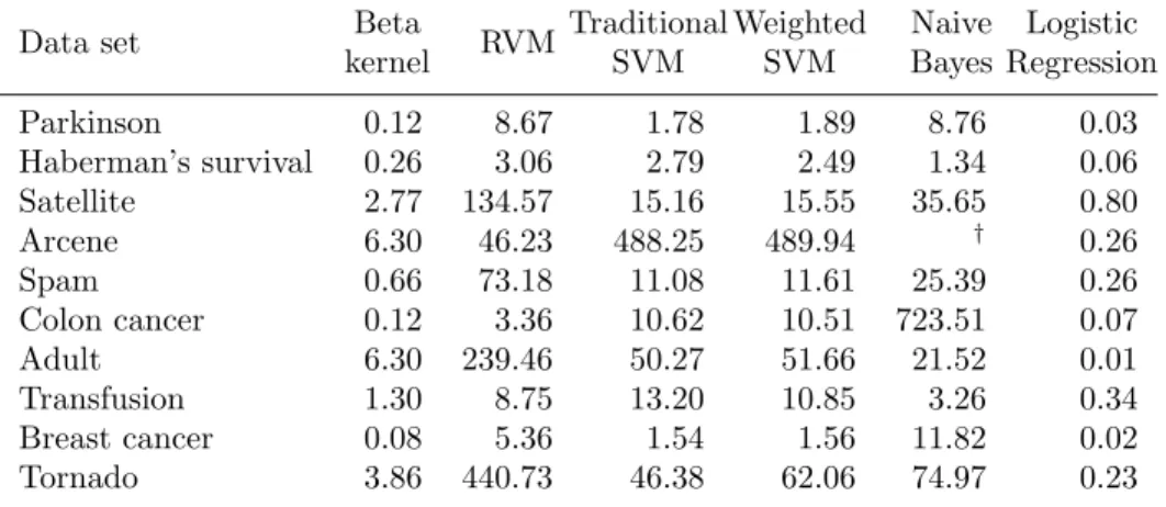
Table 3: Average run-time in seconds for binary classification models
Data set Beta RVM Traditional Weighted Naive Logistic
kernel SVM SVM Bayes Regression
Parkinson 0.12 8.67 1.78 1.89 8.76 0.03 Haberman’s survival 0.26 3.06 2.79 2.49 1.34 0.06 Satellite 2.77 134.57 15.16 15.55 35.65 0.80 Arcene 6.30 46.23 488.25 489.94 † 0.26 Spam 0.66 73.18 11.08 11.61 25.39 0.26 Colon cancer 0.12 3.36 10.62 10.51 723.51 0.07 Adult 6.30 239.46 50.27 51.66 21.52 0.01 Transfusion 1.30 8.75 13.20 10.85 3.26 0.34 Breast cancer 0.08 5.36 1.54 1.56 11.82 0.02 Tornado 3.86 440.73 46.38 62.06 74.97 0.23
† algorithm fails to terminate in a reasonable amount of time
spam with the polynomial kernel, colon cancer, breast cancer, and tornado). Two of those sets have differences in the means that are significant at the 0.1 level, and one is significant at the 0.01 level. Logistic regression has the largest AUC for three data sets, corresponding to the data sets for which it had the best average accuracy, and RVM has the highest average AUC for two data sets (arcene and spam with RBF kernel). Because SVM does not calculate probabilities, it performs worse on this metric.
We record the average run-time from the 200 different runs for each algo-rithm in Table 3. Logistic regression is the fatest algoalgo-rithm because it does not have any parameters to tune. The beta kernel’s most complicated operation is calculating the kernel matrix, and the average run-time is a few seconds. The SVM algorithms are also very fast, but the SVM algorithm has two parameters to tune (σ and C) which multiplies the number of times the SVM optimiza-tion problem is solved. Although the RVM usually relies on fewer vectors than the SVM to classify unknown data points, the RVM algorithm as developed by Tipping and Faul (2003) sequentially selects vectorsxj that are used to classify
unknown data points. This sequential process can take a long time, as with the satellite, adult, and tornado data sets. The naive Bayes algorithm takes a very long time when the data have a large number of attributes, and the arcene data
set has so many attributes that the naive Bayes algorithm does not terminate in a reasonable amount of time.
3.2. Imbalanced data sets
Imbalanced data sets can cause problems for data mining and statistical learning because algorithms like the SVM tend to classify almost all of data points in the class that occurs most frequently, the majority class (Akbani et al., 2004; Batista et al., 2004; Visa and Ralescu, 2005; Chawla, 2010). Under-sampling the majority class or over-Under-sampling the minority class so that both classes have an equal number of data points when training the algorithm can help the machine learning tool more accurately identify data points in the minority class (Maloof, 2003; Tang et al., 2009). The Synthetic Minority Over-sampling Technique (SMOTE) creates new data points through linear combinations of two input data points belonging to the minority class (Chawla et al., 2002, 2003) so that the minority class has an equivalent number of points as the majority class. These sampling techniques can be used in combination with machine learning algorithms such as the SVM and RVM (Van Hulse et al., 2007).
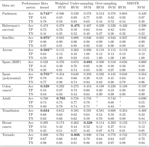
Although none of the data sets used previously have the same number of data points in both classes, we create much more imbalanced data sets from these ten data sets. We randomly select only 5% in the minority class for the eight databases. For example, the Parkinson data have 75% positively labeled and 25% negatively labeled points, and the new imbalanced Parkinson data have 95% positive and 5% negative. Conversely, 95% of the data are negatively classified and 5% are positively classified in the breast cancer data set. Because the colon cancer data only contain 62 data points, too few negatively classified data points exist to have the 19:1 ratio between the negative and positive class in a training, tuning, and testing set. Therefore, the imbalanced colon cancer data contain 10% positive and 90% negative.
The beta kernel model with the weighting parameters is compared to several other methods designed to address these heavily imbalanced data sets. In addi-tion to the weighted SVM (which was previously deployed), these other
meth-ods are under-sampling the majority class, over-sampling the minority class, and SMOTE. Each of these three sampling techniques are applied separately to the RVM and SVM. We test the eight different classifiers for the ten heavily imbalanced data sets, with the same rules as before for training, tuning, and testing. Each algorithm is tested 200 times for each data set.
With the imbalanced data, the beta kernel model performs the best in six of the eleven data trials (Table 4), and the differences in means are statistically significant at the 0.01 level for three data sets (Parkinson, arcene, and spam with the polynomial kernel). The beta kernel model’s accuracy for four other data sets compares well to the best accuracy. The beta kernel’s average accuracy is within 0.01 of the best mean accuracy for Haberman’s survival, adult, and tornado and within 0.04 for breast cancer. The beta kernel performs poorly in comparison to the other classifiers on the spam data set with the RBF kernel, but the beta kernel classifier performs much better on the same data using the polynomial kernel. Overall, under-sampling performs better than over-sampling and has the additional benefit of being faster than over-sampling or SMOTE although the beta kernel is the fastest. The mean accuracies for under-sampling with the RVM and under-sampling with the SVM are each the best for two data sets, but under-sampling with SVM performs extremely poorly for the arcene data.
3.3. Comparison of beta kernel and SVM
Comparing the performance of the beta kernel model with the SVM can shed light on situations where the beta kernel model may be more effective than the SVM. We use the twonorm data set, proposed by Breiman (1996), as the basis of this comparison but reduce the number of the attributes from the original 20 to 2 in order to plot and explain the results. Both classes are drawn from multivariate normal distributions with unit covariance matrices. The attribute means corresponding to the positive class are (0.5,0.5) and the attribute means corresponding to the negative class are (−0.5,−0.5). The beta kernel model and the SVM are compared for two training sets: (i) a training set
Table 4: Binary classification results with 5% in the minority class
Data set Performance Beta Weighted Under-sampling Over-sampling SMOTE
metric kernel SVM RVM SVM RVM SVM RVM SVM Parkinson Acc 0.743** 0.586 0.529 0.578 0.513 0.578 0.604 0.449 TP 0.81 0.85 0.69 0.77 0.95 0.92 0.92 0.97 TN 0.78 0.58 0.63 0.63 0.44 0.52 0.54 0.38 Haberman’s Acc 0.473 0.378 0.475 0.467 0.329 0.339 0.420 0.290 survival TP 0.72 0.76 0.59 0.62 0.84 0.82 0.84 0.89 TN 0.41 0.35 0.52 0.49 0.27 0.26 0.32 0.22 Satellite Acc 0.975* 0.945 0.909 0.946 0.931 0.943 0.937 0.940 TP 0.98 0.99 0.96 0.98 0.99 1.00 0.99 0.99 TN 0.97 0.91 0.88 0.92 0.92 0.90 0.89 0.91 Arcene Acc 0.502** 0.115 0.263 0.000 0.118 0.115 0.119 0.115 TP 0.64 0.12 0.42 1.00 0.12 0.12 0.12 0.12 TN 0.59 1.00 0.63 0.01 1.00 1.00 1.00 1.00 Spam (RBF) Acc 0.528 0.576 0.673 0.691 0.500 0.510 0.656 0.660 TP 0.41 0.49 0.70 0.65 0.38 0.38 0.56 0.58 TN 0.95 0.91 0.74 0.83 0.95 0.97 0.90 0.89 Spam Acc 0.755** 0.454 0.640 0.350 0.592 0.445 0.648 0.584 (polynomial) TP 0.78 0.34 0.66 0.29 0.53 0.31 0.63 0.44 TN 0.77 0.98 0.74 0.94 0.82 0.98 0.79 0.96 Colon Acc 0.529 0.292 0.273 0.454 0.198 0.220 0.189 0.197 cancer1 TP 0.55 0.37 0.73 0.60 0.20 0.23 0.20 0.20 TN 0.84 0.83 0.44 0.64 0.99 0.99 0.98 0.99 Adult Acc 0.760 0.765 0.758 0.758 † 0.743 † 0.690 TP 0.74 0.75 0.77 0.79 † 0.68 † 0.55 TN 0.80 0.79 0.74 0.75 † 0.83 † 0.89 Transfusion Acc 0.634 0.612 0.585 0.591 0.581 0.608 0.354 0.468 TP 0.68 0.63 0.62 0.64 0.54 0.58 0.22 0.32 TN 0.62 0.66 0.62 0.59 0.70 0.69 0.89 0.84 Breast Acc 0.295 0.174 0.262 0.328 0.114 0.203 0.123 0.111 cancer TP 0.54 0.42 0.44 0.52 0.12 0.27 0.14 0.12 TN 0.35 0.51 0.57 0.43 0.97 0.73 0.81 0.95 Tornado Acc 0.800 0.761 0.806 0.800 0.744 0.778 0.742 0.772 TP 0.67 0.66 0.82 0.79 0.64 0.64 0.67 0.70 TN 0.98 0.95 0.81 0.86 0.92 0.97 0.88 0.94
1Because colon cancer is a small data set, the imbalanced version has 10% positive.
** indicates the difference in accuracy with the other models is significant at the 0.01 level * indicates the difference in accuracy with the other models is significant at the 0.1 level
−3 −2 −1 0 1 2 3 −3 −2 −1 0 1 2 3
(a) Equal positive and negative
Attribute 1 Attribute 2 −2 0 2 −3 −2 −1 0 1 2 3 Attribute 1 Attribute 2 (b) Imbalanced data
Positive training data Negative training data
Beta predicts positive; SVM predicts positive Beta predicts negative; SVM predicts negative Beta predicts positive; SVM predicts negative Beta predicts negative; SVM predicts positive
Figure 1: Beta kernel and SVM classification of the twonorm data set based on (a) 30 negative and 30 positive data points in the training set and (b) 40 negative and 20 positive labeled data points in the training set
with 30 points in the negative class and 30 points in the positive class and (ii) an imbalanced training set with 40 points in the negative class and 20 points in the positive class. An unweighted SVM is used for the balanced training set, and under-sampling is used with the SVM for the second training set because this combination performed well for the imbalanced data sets in Table 4.
Fig. 1 depicts how the beta kernel model and SVM classify data ranging between -3.0 and 3.0 for each of the two attributes, given the two training data sets. The beta kernel model produces a “smoother” dividing line between the two classes for both training sets than the SVM. The beta kernel model classi-fies 6 percent more data in the minority (or positive) class for the imbalanced training set than the model does for the equally balanced training set, but the classifications based on the beta kernel model remain very similar for both train-ing sets. The SVM classifications substantially change for the two traintrain-ing sets,
and 21 percent more data are positively labeled for the equally balanced training set than in the imbalanced training set.
Because of the variation in the training data, the SVM creates areas around the positive training points for which it positively classifies unknown points and also creates areas around the negative training points for which it negatively classifies unknown points. The beta kernel model classifies unknown data points based on difference measures as determined by the RBF kernel. If an unknown data point is closer to positive points in the training set, the beta kernel model labels the unknown data point as positive and negative otherwise.
This demonstration with the twonorm data suggests that if the training data contain significant random variation, the beta kernel model may do a better job of predicting the underlying classification pattern than the SVM. For example, the SVM positively classifies a point (−1.5,0) because a point (−1.4,0.3) has a positive label in the training set, but the beta kernel model negatively classifies the point (−1.5,0) because most of the points surrounding (−1.5,0) are negatively labeled. According to the known distribution for the twonorm data set, the point (−1.5,0) has an 82 percent chance of belonging to the negative class and an 18 percent chance of belonging to the positive class. If the point (−1.4,0.3) were positively labeled because of physical reasons rather than random variations—which may signify that other points in the vicinity should also be positively classified—the SVM algorithm does a better job than the beta kernel model of uncovering that discrepancy.
3.4. Online learning
One of the principle advantages of Bayesian methods is the ability to rapidly incorporate new information into the analysis. Under Bayesian analysis, the prior distribution is updated with data, which produces a posterior distribu-tion, and that posterior distribution serves as the prior distribution in the next iteration. The Gaussian Bayesian kernel methods discussed in Section 2 are not easily adaptable to this online learning pattern because the solution algorithms generally rely on maximizing the posterior distribution. Two Gaussian Bayesian
data mining tools for online learning or incremental updating include a Bayesian online perceptron (Opper, 1998; Solla and Winther, 1998) and a sparse repre-sentation for a Gaussian process model (Csat´o and Opper, 2001). The Bayesian online perceptron approximates a posterior distribution by incrementally updat-ing mean weights and covariances for the input dataxj, but this method does
not employ kernel functions. The sparse representation for a Gaussian process model uses the kernel function as the covariance matrix as depicted in (2) and determines whether to include a new input data vectorxj based on the degree
to which the new data point changes the mean of the posterior distribution. Studying these two Bayesian classifiers for text classification reveals that they perform well in comparison with the SVM for relatively balanced classes, but SVM performs the best for imbalanced data sets (Chai et al., 2002).
The sequential RVM relies on a Bayesian Kalman filter and a least-squares approach to iteratively revise the RVM weights and hyperparameters for re-gression and time series forecasting problems (Nikolaev et al., 2005). Online or incremental learning has been investigated more fully for non-probabilistic clas-sifiers and includes algorithms such as LASVM (Bordes et al., 2005), ALMAp (Gentile, 2001), and NORMA (Kivinen et al., 2004). Jin et al. (2010) develop an algorithm that combines online learning and kernel learning which simulta-neously trains an SVM classifier and assigns weights for multiple kernels.
The beta kernel model provides an easy tool for online learning because the model does not require solving an optimization problem. The posterior dis-tribution at the end of one iteration acts as the prior disdis-tribution in the next iteration. Because the model relies on the kernel function to calculate posterior probabilities, the attributes for a data pointxi should be known although the
outcomeyiis not. The outcome remains uncertain as new data with known
out-comes are collected. For example, an oil and gas company may have geological characteristics about several different areas. As it drills for oil in certain places and discovers whether or not those places contain oil, it can update its proba-bility about whether or not a specific area contains oil based on the geological similarity between the known and unknown areas.
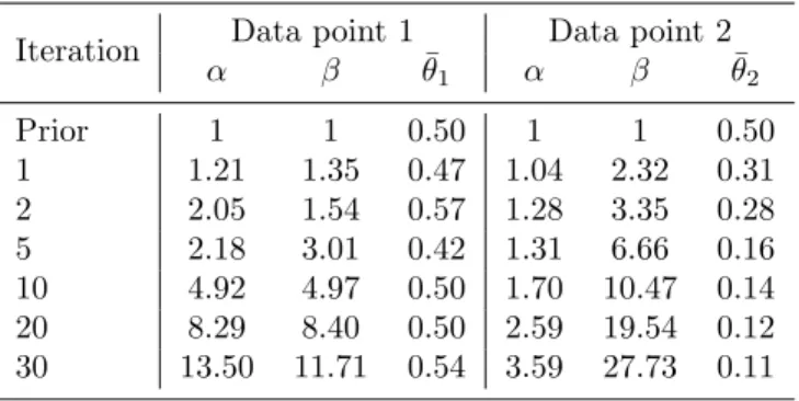
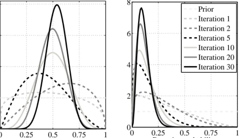
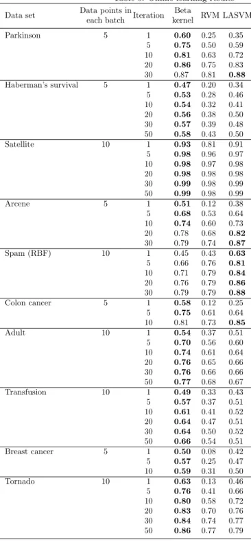
Table 5: Updated parameters for beta kernel model with twonorm data
Iteration Data point 1 Data point 2
α β θ¯1 α β θ¯2 Prior 1 1 0.50 1 1 0.50 1 1.21 1.35 0.47 1.04 2.32 0.31 2 2.05 1.54 0.57 1.28 3.35 0.28 5 2.18 3.01 0.42 1.31 6.66 0.16 10 4.92 4.97 0.50 1.70 10.47 0.14 20 8.29 8.40 0.50 2.59 19.54 0.12 30 13.50 11.71 0.54 3.59 27.73 0.11
We explore the application of the beta kernel model to online learning by (1) demonstrating howα,β, andθchange as new data arrive and (2) comparing the beta kernel’s accuracy to two other online learning tools. We depict how the beta kernel model’s parameters change using the twonorm data set as downloaded from the Delve project (Revow 1996) at the University of Toronto. Unlike the previous example, this experiment keeps all 20 attributes for the twonorm data. Although the original data set has an equal number of positively and negatively labeled outcomes, we purposely imbalance the data so that only 25% of the outcomes are positive.
We select two data points for which we assume the attributes but not the outcomes are known. At each iteration, a unique set of 10 data points whose out-comes are known is used to updateαandβfor the each of the two unknown data points whereαi =α+P{j|yj=1}k(xi,xj) andβi =β+
P
{j|yj=−1}k(xi,xj).
Table 5 depicts the updated α and β and the expected posterior probability ¯
θi = E[P(yi = 1)]. Fig. 2 displays the beta distribution’s probability density
function asαandβ are updated for each of these two data points.
As the classifier receives more information, the first data point is much more likely to result in a positive outcome than the second data point. The expected probability for the first data point is close to 0.5 during all the iterations. Even after 30 iterations, the beta distribution’s density function (the dark solid line in Fig. 2a) is still wide enough that the posterior probability could be between 0.25 and 0.75. The first data point’s expected probability is 0.54. Much uncertainty
0 0.25 0.5 0.75 1 0 1 2 3 4 Posterior probability
Probability density function
(a) Data point 1
0 0.25 0.5 0.75 1 0 2 4 6 8 Posterior probability (b) Data point 2 Prior Iteration 1 Iteration 2 Iteration 5 Iteration 10 Iteration 20 Iteration 30
Figure 2: Posterior probability distributions for two different data points in the twonorm data set
exists over whether this data point is positively or negatively labeled; however, the posterior probability is much greater than 0.25, the fraction of positively labeled data points in the data set.
Updating the parameters for the second data point significantly reduces the uncertainty of this data point’s outcome. After only 5 iterations or 50 data points, the expected probability is 0.16. After 30 iterations, the expected probability is only 0.11, and most of the beta distribution’s density function is less than 0.25.
3.5. Online learning comparison
We compare the ability of three algorithms to correctly classify data incre-mentally. The weighted beta kernel model begins with a uniform prior where α=β = 1, and these parameters and the weights for imbalanced data are up-dated with the arrival of each new set of data. Because the sequential RVM is designed for regression as opposed to classification problems, we slightly modify the standard RVM algorithm (Tipping, 2009) so that it learns incrementally. The set of vectors with non-zero weights after one iteration is assumed to have
non-zero weights with the arrival of a new batch of data, and only data in the new batch can be added to the set of vectors with non-zero weights. Once a data point is excluded from this set, it is discarded. The third algorithm is LASVM, an online SVM algorithm (Bordes et al., 2005).
We use the ten databases that were described in Section 3.1 but randomly divide each data set into batches, where each batch contains either 5 or 10 data points, depending on size of the data set. Five data sets have 50 different batches, three data sets have 30 batches, and the colon cancer and breast cancer data only have 10 batches because these latter sets contain a fewer data. At each iteration, each algorithm incorporates a new batch to classify unknown points in the testing set. Any data point not in a batch is in the testing set. The experiment is repeated 200 times for each data set.
The median optimal values that were generated by the initial binary classi-fication numerical experiments were used forσin the RBF kernel andCin the SVM for this online learning experiment. Table 6 depicts the average accuracy (the square root of the product of the TP and TN rates) for different iterations. Because online learning typically does not begin with a large training set that can be used to generate optimal parameters for kernel functions, algorithms have been developed that linearly combine multiple kernels for a single classi-fier. As the classifier learns on data, the weights for each possible kernel are also updated to improve accuracy (Jin et al., 2010; Gosselin et al., 2011). Fu-ture research could apply these concepts to the beta kernel model in an online learning environment.
After 30 iterations, the three algorithms generally return accuracies consis-tent with the mean accuracies depicted in Table 2. After 1 or 5 iterations, the beta kernel outperforms the other two algorithms except on the spam data, but LASVM’s accuracy exceeds that of the beta kernel by the 30th or 50th iteration for Parkinson, arcene, colon cancer, as well as spam. This result suggests that the beta kernel is a better algorithm than LASVM for a handful of data points
Table 6: Online learning results
Data set Data points inIteration Beta RVM LASVM each batch kernel
Parkinson 5 1 0.60 0.25 0.35 5 0.75 0.50 0.59 10 0.81 0.63 0.72 20 0.86 0.75 0.83 30 0.87 0.81 0.88 Haberman’s survival 5 1 0.47 0.20 0.34 5 0.53 0.28 0.46 10 0.54 0.32 0.41 20 0.56 0.38 0.50 30 0.57 0.39 0.48 50 0.58 0.43 0.50 Satellite 10 1 0.93 0.81 0.91 5 0.98 0.96 0.97 10 0.98 0.97 0.98 20 0.98 0.98 0.98 30 0.99 0.98 0.99 50 0.99 0.98 0.99 Arcene 5 1 0.51 0.12 0.38 5 0.68 0.53 0.64 10 0.74 0.60 0.73 20 0.78 0.68 0.82 30 0.79 0.74 0.87 Spam (RBF) 10 1 0.45 0.43 0.63 5 0.66 0.76 0.81 10 0.71 0.79 0.84 20 0.76 0.79 0.86 30 0.79 0.79 0.88 Colon cancer 5 1 0.58 0.12 0.25 5 0.75 0.61 0.64 10 0.81 0.73 0.85 Adult 10 1 0.54 0.37 0.51 5 0.70 0.56 0.60 10 0.74 0.61 0.64 20 0.76 0.65 0.66 30 0.76 0.66 0.66 50 0.77 0.68 0.67 Transfusion 10 1 0.49 0.33 0.43 5 0.57 0.37 0.51 10 0.61 0.41 0.52 20 0.64 0.47 0.51 30 0.64 0.50 0.52 50 0.66 0.54 0.51 Breast cancer 5 1 0.50 0.08 0.42 5 0.57 0.25 0.47 10 0.59 0.31 0.50 Tornado 10 1 0.63 0.13 0.46 5 0.76 0.41 0.66 10 0.80 0.58 0.72 20 0.83 0.70 0.76 30 0.84 0.74 0.77 50 0.86 0.77 0.79
(i.e., less than 50). When the data set contains more than 50 data points, the beta kernel and LASVM perform comparably, which echoes the findings from Table 2 in which the beta kernel and SVM algorithms perform similarly. In the online learning environment, the beta kernel model outperforms LASVM for the Haberman’s survival, satellite, adult, transfusion, breast cancer, and tor-nado data sets after 30 or 50 iterations (which correspond to 150 to 500 data points). Although not shown in the table, the beta kernel runs more quickly than the RVM and LASVM.
4. Conclusions
This paper has explored the usefulness of the beta kernel model and com-pared the model’s accuracy with the RVM (a binary classification algorithm based on Gaussian distributions), the SVM, naive Bayes, and logistic regres-sion. The beta kernel model relies on the well-known beta-binomial Bayesian formula, and deploying a kernel function as a measure of similarity between two different data points enables us to apply these updating techniques to clas-sification problems. Incorporating weighting parameters or beginning with a non-uniform prior can help the model correctly classify imbalanced data sets. The model can be generalized to a Dirichlet kernel model for multiclass classifi-cation problems, and future research can compare the accuracy of the Dirichlet kernel model with other multiclass classifiers.
The extensive numerical testing of the beta kernel model with the RVM, SVM, naive Bayes, and logistic regression indicates that the beta kernel model may have some advantages that can be exploited for classification problems. The beta kernel model performs similarly to the SVM, a weighted SVM, and logistic regression for the ten data sets in which the minority class composes between 7 and 44% of the data. The beta kernel model consistently performs better
than the RVM and naive Bayes. If the user desires a probabilistic data mining tool, the beta kernel model may be a superior choice to the RVM. When the minority class comprises only 5% of the data, the beta kernel model is usually more accurate than the RVM and SVM, even though the latter two classifiers were improved using under-sampling, over-sampling, and SMOTE. This suggests that the beta kernel model should be an important tool for classifying heavily imbalanced data sets. The online learning experiment reveals that the beta kernel model consistently outperforms the RVM and LASVM (an incremental learning version of the SVM) if 50 or fewer data points are available, and the model frequently performs better than the RVM and LASVM even if more data are available. Finally, the beta kernel model calculates posterior probabilities very quickly and runs faster than the RVM and SVM, both of which rely on solving optimization problems.
As this paper represents, to our knowledge, the first extensive analysis and testing of the beta kernel model, we believe the model can potentially become a useful tool in machine learning. The beta kernel model provides similar accu-racies for classifying data sets where the number in each class is relatively the same, and the model carries other advantages, such as fast computation times. If the data set is heavily imbalanced, the beta kernel model may be the most accurate. If the data arrive incrementally, the model easily and quickly updates to incorporate the new data and can be relatively accurate with just a few data points. Future work could explore if the beta kernel model can be combined with the SVM, RVM, and logistic regression to improve overall accuracy. We intend to apply the beta kernel model to existing problems and demonstrate how some of these benefits can aid a decision maker.
Appendix
We seek to prove that the uniform beta prior with a weighted kernel like-lihood will label an unknown data point as a beta prior that derives from the training set and is updated with an unweighted kernel likelihood.
The uniform prior (α = β = 1) and weighted kernel likelihood labels an unknown pointxi in the positive class if and only if (14) holds.
1 + m− m Pk+ ij 2 + m− m P kij++m+ m P kij− >0.5 (14) We assign Pk+ ij = P {j|yj=1}k(xi,xj) and Pk− ij = P {j|yj=−1}k(xi,xj) for notational convenience.
If the prior is formulated so that the prior’s expected value is the proportion of positively labeled points in the training set, then an unknown point will be positively classified if and only if (15) holds.
P k+ij P kij++P kij− > m+ m (15)
We want to show that (14) and (15) are equivalent. We begin with (14).
1 + m− m P k+ij > 1 + 0.5 m− m P kij++m+ m P kij− m−Pk+ij > 0.5 m− P k+ij+m+Pkij− 0.5m−Pk+ij > 0.5m+Pkij− m−Pkij++m+Pk+ij > m+Pkij−+m+Pk+ij mPk+ ij > m+ Pkij−+ Pk+ ij (16)
Acknowledgements
This work was funded in part by the U.S. Army Research, Development and Engineering Command, Army Research Office, Mathematical Sciences Division, under proposal no. 61414-MA-II.
References
Akbani, R., Kwek, S., & Japkowicz, N. (2004). Applying support vector ma-chines to imbalanced datasets. In J.-F. Boulicaut, F. Esposito, F. Giannotti, & D. Pedreschi (Eds.), Machine learning: ECML 2004 (pp. 39-50). Berlin: Springer.
Alon, U., Barkai, N., Notterman, D. A., Gish, K., Ybarra, S., Mack, D., & Levine, A. J. (1999). Broad patterns of gene expression revealed by clustering of tumor and normal colon tissues probed by oligonucleotide arrays. Proceed-ings of the National Academy of Sciences, 96, 6745-6750, http://genomics-pubs.princeton.edu/oncology/affydata/index.html. Accessed 4 April 2011. Bache, K., & Lichman, M. (2013). UCI Machine Learning Repository School
of Information and Computer Science, University of California, Irvine http://archive.ics.uci.edu/ml. Accessed 11January 2014.
Batista, G. E. A. P. A., Prati, R. C., & Monard, M. C. (2004). A study of the behavior of several methods for balancing machine learning training data. SIGKDD Explorations, 6(1), 20-29.
Bishop, C. M., & Tipping, M. E. (2003). Bayesian regression and classification. In J. A. K. Suykens, G. Horv´ath, S. Basu, C. Micchelli, & J. Vandewalle (Eds.), Advances in learning theory: Methods, models and applications (pp. 267-288). Amsterdam: IOS Press.
Bordes, A., Ertekin, S., Weston, J., & Bottou, L. (2005). Fast kernel classifiers with online and active learning. Journal of Machine Learning Research, 6, 1579-1619.
Breiman L. (1996).Bias, variance and arcing classifiers. Technical Report 460, Statistics department. University of California. April.
Carlin, B. P., & Louis, T. A. (2008).Bayesian Methods for Data Analysis, 3rd ed. Boca Raton, FL: CRC Press.
Chai, K. M. A., Ng, H. T., & Chieu, H. L. (2002). Bayesian online classifiers for text classification and filtering. Paper presented at the SIGIR, Tampere, Finland. August 11-15.
Chang, C.-C., & Lin, C.-J. (2001). LIBSVM: A library for support vector ma-chines. Software available at http://www.csie.ntu.edu.tw/∼cjlin/libsvm. Chapelle, O. (2005). Active learning for Parzen window classifier. InProceedings
of the 10th international workshop on artificial intelligence and statistics, Bar-bados. http://olivier.chapelle.cc/pub/aistats05.pdf. Accessed 4 April 2011. Chawla, N. V. (2010). Data mining for imbalanced datasets: An overview. In O.
Maimon & L. Rokach (Eds.),Data Mining and Knowledge Discovery Hand-book(2 ed., pp. 875-886). New York: Springer Science.
Chawla, N. V., Bowyer, K. W., Hall, L. O., & Kegelmeyer, W. P. (2002). SMOTE: Synthetic minority over-sampling technique. Journal of Artificial Intelligence Research, 16, 321-357.
Chawla, N. V., Lazarevic, A., Hall, L. O., & Bowyer, K. W. (2003). SMOTE-Boost: Improving prediction of the minority class in boosting. Paper pre-sented at the 7th European Conference on Principles and Practice of Knowl-edge Discovery in Databases (PKDD), Dubrovnik, Croatia.
Chew, H.-G., Crisp, D. J., Bogner, R. E., & Lim, C.-C. (2000). Tar-get detection in radar imagery using support vector machines with training size biasing. In Proceedings of the 6th international conference on control, automation, robotics, and vision, Singapore. http://kernel-machines.org/papers/upload 11483 ICARCV2000-4.ps. Accessed 5 April 2011.
Cristianini, N., & Shawe-Taylor, J. (2000). An introduction to support vector machines and other kernel-based learning methods. Cambridge: Cambridge University Press.
Csat´o, L., & Opper, M. (2001). Sparse representation for Gaussian process models. In T. K. Leen, T. G. Dietterich & V. Tresp (Eds.),NIPS 2000 (Vol. 13): MIT Press.
Figueiredo, M. A. T. (2002). Adaptive sparseness using Jeffreys prior. In T. Dietterich, S. Becker, & Z. Ghahramani (Eds.),Neural information processing systems, (Vol. 14, pp. 697-704). Cambridge: MIT Press.
Foody, G. M. (2008). RVM-based multi-class classification of remotely sensed data.International Journal of Remote Sensing, 29(6), 1817-1823.
Gentile, C. (2001). A new approximate maximal margin classification algorithm. Journal of Machine Learning Research, 2, 213-242.
Gosselin, P. H., Precioso, F., & Philipp-Foliguet, S. (2011). Incremental kernel learning for active image retrieval without global dictionaries.Pattern Recog-nition, 44(10-11), 2244-2254.
Gupta, A. K., & Nadarajah, S. (Eds.) (2004).Handbook of beta distribution and its applications. New York: Marcel Dekker.
Guyon, I., Gunn, S. R., Ben-Hur, A., & Dror, G. (2004). Result analysis of the NIPS 2003 feature selection challenge. In Neural Information Processing Sys-tem. http://books.nips.cc/papers/files/nips17/NIPS2004 0194.pdf (Accessed May 4, 2012).
Haberman, S. J. (1976). Generalized residuals for log-linear models.Proceedings of the 9th International Biometrics Conference, Boston, 104-122.
Hastie, T., Tibshirani, R., & Friedman, J. (2001). The elements of statistical learning: Data mining, inference, and prediction. New York: Springer Science. Huang, S.-C., & Wu, T.-K. (2008). Combining wavelet-based feature extractions with relevance vector machines for stock index forecasting. Expert Systems, 25(2), 133-149.
Jin, R., Hoi, S. C. H., & Yang, T. (2010). Online multiple kernel learning: Algorithms and mistake bounds.Algorithmic Learning Theory, 6331, 390-404. King, G., & Zeng, L. (2001). Logistic regression in rare events data. Political
Analysis, 9, 137-163.
Kivinen, J., Smola, A. J., & Williamson, R. C. (2004). Online learning with kernels.IEEE Transactions on Signal Processing, 52(8), 2165-2176.
Kohavi, R. (1996). Scaling up the accuracy of Naive-Bayes classifiers: a decision-tree hybrid. In E. Simoudis, J. Han, & U. Fayyad (Eds.),Proceedings of the Second International Conference on Knowledge Discovery and Data Mining (pp. 202-207). http://robotics.stanford.edu/ ronnyk/nbtree.pdf. Accessed 11 January 2014.
Kubat, M., Holte, R., & Matwin, S. (1997). Learning when negative examples abound. In M. van Someren & G. Widmer (Eds.),Machine learning,
ECML-97: Proceedings of the 9th European conference on machine learning (pp. 146-153). Heidelberg: Springer.
Kudo, T., & Matsumoto, Y. (2003). Fast methods for kernel-based text anal-ysis. In Hinrichs, E. W., & Roth, D. (Eds.), Proceedings of the 41st An-nual Meeting of the Association for Computational Linguistics (pp. 24-31), July. Stroudsburg, PA: Association for Computational Linguistics. http://acl.ldc.upenn.edu/acl2003/main/pdfs/Kudo.pdf. Accessed 6 January 2014.
Little, M. A., McSharry, P. E., Hunter, E. J., Spielman, J., & Ramig, L. O. (2009). Suitability of dysphonia measurements for telemonitoring of Parkin-son’s disease. IEEE Transactions on Biomedical Engineering, 56(4), 1015-1022.
Maloof, M. A. (2003). Learning when data sets are imbalanced and when costs are unequal and unknown. Paper presented at the International Conference on Machine Learning Workshop on Learning from Imbalanced Data Sets, Washington, DC.d
Maalouf, M., & Trafalis, T. B. (2008). Kernel logistic regression using truncated Newton method. In C. H. Dagli, D. L. Enke, K. M. Bryden, H. Ceylen, & M. Gen (Eds.),Intelligent engineering systems through artificial neural networks, Vol. 18 (pp. 455-462). New York: ASME Press.
Maalouf, M., & Trafalis, T. B. (2011). Robust weighted kernel logistic regres-sion in imbalanced and rare events data.Computational Statistics and Data Analysis, 55, 168-183.
Mallick, B. K., Ghosh, D., & Ghosh, M. (2005). Bayesian classification of tu-mours by using gene expression data.Journal of the Royal Statistical Society, Part B, 67(2), 219-234.
Mason, M., & Lopes, M. (2011). Robot self-initiative and personaliza-tion by learning through repeated interacpersonaliza-tions. In Proceedings of the 6th ACM/IEEE international conference on human-robot interaction (HRI’11), Lausanne, Switzerland. http://flowers.inria.fr/mlopes/myrefs/11-hri.pdf. Ac-cessed 5 April 2011.
Matlab (2012). NaiveBayes.fit. Version R2012b. Mathworks.
Moon, J., Shon, T., Seo, J., Kim, J., & Seo, J. (2004). An approach for spam e-mail detection with support vector machine and n-gram indexing. In Aykanat, C., Dayar, T., & K orpeo˘gu, ˙I, eds. Computer and Information Sciences -ISCIS 2004: 19th International Symposium (pp. 351-362), Kemer-Antalya, Turkey. Berlin: Springer.
Montesano, L., & Lopes, M. (2009). Learning grasping affordances from local visual descriptors. InProceedings of the 8th IEEE international conference on development and learning, Shanghai, China.
Morik, K., Brockhausen, P., & Joachims, T. (1999). Combin-ing statistical learning with a knowledge-based approach–a case study in intensive care monitoring. In Proceedings of the 16th international conference on machine learning, Bled, Slovenia.
http://citeseerx.ist.psu.edu/viewdoc/download?doi=10.1.1.71.5781&rep=rep1&type=pdf. Accessed 4 April 2011.
Nikolaev, N., & Tino, P. (2005). Sequential relevance vector machine learning from time series. Paper presented at the International Joint Conference on Neural Networks, Montreal, Canada. July 31 - August 4.
Opper, M. (1998). A Bayesian approach to online learning. In D. Saad (Ed.), On-Line Learning in Neural Networks(pp. 363-378). New York: Cambridge University Press.
Parzen, E. (1962). On estimation of a probability density function and mode. The Annals of Mathematical Statistics, 33(3), 1065-1076.
Revow, M. (1996). Twonorm data set. Delve datasets.
http://www.cs.toronto.edu/˜delve/data/twonorm/desc.html. Accessed 8 May 2012.
Saha, B., Goebel, K. & Christophersen, J. (2009). Comparison of prognostic algorithms for estimating remaining useful life of batteries.Transactions of the Institute of Measurement and Control, 31(3/4), 293-308.
Sch¨olkopf, B., & Smola, A. J. (2002). Learning with kernels: Support vector machines, regularization, optimization, and beyond. Cambridge: MIT Press. Seeger, M. (2000). Bayesian model selection for support vector machines,
Gaus-sian processes and other kernel classifiers. In S. A. Solla, T. K. Leen, & K.-R. M¨uller (Eds.), Advances in neural information processing systems(pp. 603-609). Cambridge: MIT Press.
Shawe-Taylor, J. & Cristianini, N. (2004).Kernel methods for pattern analysis. Cambridge: Cambridge University Press.
Solla, S. A., & Winther, O. (1998). Optimal perceptron learning: An online Bayesian approach. In D. Saad (Ed.), On-Line Learning in Networks (pp. 379-399). New York: Cambridge University Press.
Street, W. N., Mangasarian, O. L., & and Wolberg, W. H. (1995). An inductive learning approach to prognostic prediction. In A. Prieditis & S. Russell (Eds.), Proceedings of the Twelfth International Conference on Machine Learning (pp. 522-530), San Francisco: Morgan Kaufmann.
for highly imbalanced classification. IEEE Transactions on Systems, Man, and Cybernetics, Part B: Cybernetics, 39(1), 281-288.
Tipping, M. E. (2001). Sparse Bayesian learning and the relevance vector ma-chine.Journal of Machine Learning Research, 1, 211-244.
Tipping, M. E. (2009). SparseBayes for Matlab, version 2.
http://www.vectoranomaly.com/downloads/downloads.htm. Accessed 4 April 2011.
Tipping, M. E. & Faul, A. C. (2003). Fast marginal likelihood maximisation for sparse Bayesian models. In C. M. Bishop and B. J. Frey (Eds.),Proceedings of the 9th international workshop on artificial intelligence and statistics, Key West, Florida. http://www.miketipping.com/papers.htm. Accessed 4 April 2011.
Trafalis, T. B., Adrianto, I., & Richman, M. B. (2007). Active learning with sup-port vector machines for tornado prediction. In Y. Shi, G. D. van Albada, J. Dongarra, & P. M. A. Sloot (Eds.),Computational science–ICCS 2007: Pro-ceedings of the 7th international conference on computational scienceBeijing, China (pp. 1130-1137). Berlin: Springer-Verlang.
Van Hulse, J., Khoshgoftaar, T. M., & Napolitano, A. (2007). Experimental Perspectives on Learning from Imbalanced Data. Paper presented at the 24th International Conference on Machine Learning, Corvallis, OR, 935-942. Visa, S., & Ralescu, A. (2005). Issues in mining imbalanced data sets–A review
paper. Paper presented at the Proceedings of Midwest Artificial Intelligence and Cognitive Science Conference (MAICS ’05), Dayton.
Wang, B. X., & Japkowicz, N. (2008). Boosting support vector machines for imbalanced data sets. In A. Aijun, S. Matwin, Z. W. Ra´s, & D. ´Sl¸ezak (Eds.),
Foundations of intelligent systems: Proceedings of the 17th international sym-posium on methodologies for intelligent systems, Toronto, Canada (pp. 38-47). Berlin: Springer-Verlag.
Wang, S., Jiang, W., & Tsui, K.-L. (2010). Adjusted support vector machines based on a new loss function.Annals of Operations Research 174:83-101. Yeh, I-C., Yang, K.-J., & Ting, T.-M. (2009). Knowledge discovery on RFM
model using Bernoulli sequence. Expert Systems with Applications, 36(3), 5866-5871.
Zhang, Z., Dai, G., & Jordan, M. I. (2011). Bayesian generalized kernel mixed models.Journal of Machine Learning Research, 12, 111-139.