This is a repository copy of
Multilayer Probability Extreme Learning Machine for
Device-Free Localization
.
White Rose Research Online URL for this paper:
http://eprints.whiterose.ac.uk/142336/
Version: Accepted Version
Article:
Zhang, J, Xiao, W, Li, Y et al. (2 more authors) (2019) Multilayer Probability Extreme
Learning Machine for Device-Free Localization. Neurocomputing. ISSN 0925-2312
https://doi.org/10.1016/j.neucom.2018.11.106
© 2019, Elsevier B.V. This manuscript version is made available under the CC-BY-NC¬ ND
4.0 license http://creativecommons.org/licenses/by-nc-nd/4.0/.
Reuse
This article is distributed under the terms of the Creative Commons Attribution-NonCommercial-NoDerivs (CC BY-NC-ND) licence. This licence only allows you to download this work and share it with others as long as you credit the authors, but you can’t change the article in any way or use it commercially. More
information and the full terms of the licence here: https://creativecommons.org/licenses/
Takedown
If you consider content in White Rose Research Online to be in breach of UK law, please notify us by
Multilayer Probability Extreme Learning Machine for Device-Free Localization
Jie Zhanga,b, Wendong Xiaoa,b,∗, Yanjiao Lia,b, Sen Zhanga,b, Zhiqiang ZhangcaSchool of Automation&Electrical Engineering, University of Science and Technology Beijing, Beijing 100083, China bBeijing Engineering Research Center of Industrial Spectrum Imaging, Beijing 100083, China
cSchool of Electronic and Electrical Engineering, University of Leeds, Leeds LS2 9JT, UK
Abstract
Device-free localization (DFL) is becoming one of the new techniques in wireless localization field, due to its advan-tage that the target to be localized does not need to attach any electronic device. One of the key issues of DFL is how to characterize the influence of the target on the wireless links, such that the target’s location can be accurately estimated by analyzing the changes of the signals of the links. Most of the existing related research works usually extract the useful information from the links through manual approaches, which are labor-intensive and time-consuming. Deep learning approaches have attempted to automatically extract the useful information from the links, but the training of the conventional deep learning approaches are time-consuming, because a large number of parameters need to be fine-tuned multiple times. Motivated by the fast learning speed and excellent generalization performance of extreme learning machine (ELM), which is an emerging training approach for generalized single hidden layer feedforward neu-ral networks (SLFNs), this paper proposes a novel hierarchical ELM based on deep learning theory, named multilayer probability ELM (MP-ELM), for automatically extracting the useful information from the links, and implementing fast and accurate DFL. The proposed MP-ELM is stacked by ELM autoencoders, so it also keeps the very fast learn-ing speed of ELM. In addition, considerlearn-ing the uncertainty and redundant links existlearn-ing in DFL, MP-ELM outputs the probabilistic estimation of the target’s location instead of the deterministic output. The validity of the proposed MP-ELM-based DFL is evaluated both in the indoor and the outdoor environments, respectively. Experimental results demonstrate that the proposed MP-ELM can obtain better performance compared with classic ELM, multilayer ELM (ML-ELM), hierarchical ELM (H-ELM), deep belief network (DBN), and deep Boltzmann machine (DBM). Keywords: Device-Free Localization, Extreme Learning Machine, Extreme Learning Machine Autoencoder, Multilayer Probability Extreme Learning Machine
1. Introduction
In the past decade, the widespread usage of mobile devices in the daily life has promoted the rapid development of location-based service. Hence, many localization techniques have been explored, such as wearable device, infrared sensor, and video surveillance, etc. However, those techniques require the localized entity to attach additional elec-tronic devices or involve personal privacy, which limit their application to some extent [1, 2, 3, 4]. In order to tackle
5
the above issues, device-free localization (DFL) was introduced as a new radio frequency (RF)-based localization approach, where the target does not need to attach any electronic device [5]. DFL can be applied to both indoor and outdoor environments, and is particularly useful in smoky, dark, and obscure scenarios, which makes it an attractive and promising technique for a variety of applications [6]. In a DFL system, radio transmitters (RTs) and radio receiver-s (RXreceiver-s) are ureceiver-sed areceiver-s the receiver-senreceiver-sor nodereceiver-s to receiver-senreceiver-se the target collaboratively. Areceiver-s the original receiver-signal field will be changed
10
when the target enters the monitoring area, the target’s location can be estimated through analyzing the changes of the signals, such as the differential received signal strength (RSS) measurements, of the corresponding links in the wireless network. In the monitoring area, theoretically, if there aresfixed sensor nodes placed along its boundary, the
∗Corresponding author
ssensor nodes will provides(s−1)/2 different wireless links in total. Among the links of the deployed sensor nodes, many links are useless and redundant, and some of them even may degrade the localization accuracy. Thus, how to
15
extract the useful information from the links is the key to accurately estimate the target’s location. In the past decade, in order to tackle this issue, many research works have tried to propose different manual feature extraction approaches to characterize the RSS of the links [7]. Accordingly, for different scenarios, it is hard to directly determine which links are absolutely more useful or useless. Thus, usually, lots of time and effort are consumed in manually extracting useful information for the specific problems. Motivated by its excellent performance in extracting features, some
20
researchers applied deep learning approach to DFL to automatically determine discriminative features. For example, Wang et al. [8] proposed a deep sparse autoencoder to project the high-dimensional RSS data to low-dimensional feature, and obtained satisfactory performance. However, the conventional deep learning approaches, such as deep Boltzmann machine (DBM), and deep belief network (DBN), suffer from the time-consuming training process, be-cause a large number of parameters need to be fine-tuned multiple times. Therefore, it is worthwhile to study how to
25
apply new deep learning approach to implement fast and accurate DFL.
Different from most of the existing machine learning approaches, such as back propagation neural network (BPN-N) and support vector machine (SVM), extreme learning machine (ELM) is a new training algorithm for the single hidden layer feedforward neural networks (SLFNs) [9]. The salient feature of ELM is that its hidden layer parameters are generated randomly in advance and only the output weights are required to be calculated through the least-square
30
approach, so it can obtain much faster learning speed and better generalization performance [10]. In addition, ELM also overcomes some issues faced in most of the machine learning approaches, such as local minimum, predefining of learning rate and stopping criterion [11]. Due to the above advantages, ELM has been widely used in many real ap-plications, such as industrial production [12], localization [13], finite-time optimal control of nonlinear systems [14], solar radiation perdiction [15], etc. Theoretically, ELM has been extended to online learning [16], semi-supervised
35
and unsupervised learning [17, 18], ensemble learning [19], imbalance learning [20, 21, 22], and residual learning [23], etc. Furthermore, considering the above shallow ELMs still face some challenges in dealing with complex tasks [24], such as image classification, voice recognition, and natural language processing, some researchers proposed hi-erarchical ELMs based on deep learning theory, including multilayer ELM (ML-ELM), stacked ELM (S-ELM), and hierarchical ELM (H-ELM), etc.
40
Considering the advantages of ELM and complexity of DFL, in this paper, we will propose a novel hierarchical ELM based on deep learning theory, named multilayer probability ELM (MP-ELM), which is stacked by ELM au-toencoders (ELM-AE), for automatically extracting the useful information from the links, and implementing fast and accurate DFL. We evaluate the proposed MP-ELM-based DFL both in the indoor and the outdoor environments, by comparing it with classic ELM, ML-ELM, H-ELM, DBN, and DBM. Experimental results demonstrate that the
pro-45
posed MP-ELM can obtain better performance. The main contributions of this paper can be summarized as follows: 1) A novel hierarchical ELM with probabilistic output is proposed, i.e., MP-ELM. The proposed MP-ELM consists of two phases, including the unsupervised feature representation phase and the supervised decision making phase. In the unsupervised feature representation phase, ELM-AE is implemented at each layer for extracting the useful feature layer by layer iteratively; and for the supervised decision making phase, an output layer with probabilistic estimation
50
based on the sigmoid function is performed for the final decision making, which can avoid overfitting with better generalization performance and is more robust.
2) Different from the conventional deep learning approaches stacked by BP-based AE, ELM-AEs in MP-ELM make parameter fine-tuning not necessary in its training phase, so the learning speed of MP-ELM can be much faster. 3) The proposed MP-ELM can automatically extract useful information from the links, which not only can avoid
55
the labor-intensive and time-consuming feature exploration procedure in the conventional DFL approaches, but also can extract more representative features with discriminative capability than the handcraft ones. In addition, consider-ing the uncertainty of DFL, MP-ELM outputs the probability distribution of target’s location instead of fittconsider-ing to data, which converts the original solid classification to soft classification, and achieve better accuracy.
The paper is organized as follows. Related work is illustrated in Section 2. Preliminaries are introduced in
60
Section 3, including the brief introduction of ELM theory and ELM-AE. Section 4 details the MP-ELM-based target’s location estimation, including the motivation of proposing a hierarchical ELM with probabilistic output for DFL, the main framework of MP-ELM-based DFL, and the detailed MP-ELM. Experimental results and further analysis are reported in Section 5, followed by discussions in Section 6. Finally, conclusions and future work are given in Section 7.
2. Related Work
In this section, we will briefly introduce the related works of hierarchical ELMs and device-free localization, respectively.
2.1. Hierarchical ELMs based on Deep Learning Theory
As mentioned above, in order to deal with complex tasks, such as image classification, vioce recognition, and
70
natural language processing, ELM has been extended to hierarchical structure based on deep learning theory. Kasun et al. [25] attempted to a multilayer architecture using ELM autoencoder (ELM-AE) as its building block (multilayer ELM, ML-ELM), but the proposed ELM-AE requires the weights and biases to be orthogonal, which cannot guarantee the ELM’s universal approximation capability. For solving large and complex tasks using ELM without incurring the memory problem, Zhou et al. [26] proposed stacked ELMs (S-ELM) with multilayer structure based on the principal
75
component analysis (PCA), which could achieve better performance with small memory requirement. As ML-ELM cannot guarantee the universal approximation of ELM, Tang et al. [27] proposed a hierarchical ELM (H-ELM) based on a L1-norm ELM-AE. Due to the use of L1 penalty, the new ELM-AE can obtain more sparse and meaningful features, and the proposed H-ELM could achieve better performance and much faster convergence speed than some conventional deep learning approaches. Different from the aforementioned ELM-AEs, Zhang et al. [28] introduced
80
a local denoising criterion to ELM-AE and proposed ELM denoising autoencoder (ELM-DAE), which can extract higher level features. Accordingly, they designed denoising Laplacian multilayer ELM (D-Lap-ML-ELM) based on ELM-DAE, which could obtain good performance in dealing with supervised learning problems. In addition, Sun et al. [29] combined ELM-AE with manifold regularization and proposed generalized ELM-AE (GELM-AE), which has better representation capability for clustering. Recently, a kernel version of ML-ELM was proposed for eliminating
85
the manual tuning and guaranteeing the generalization performance [30]. 2.2. Device-Free Localization
In the past decade, different kinds of approaches have been proposed for DFL, mainly including fingerprinting and machine learning approaches, radio tomographic imaging (RTI) approach, compressive sensing (CS) approach, and geometric approach, etc.
90
Fingerprinting approach for DFL mainly involves two phases, i.e., the offline phase and the online phase [31]. An accurate radio map is the key for obtaining good localization accuracy, which is created in the offline phase by recording the differential received signal strength (RSS) measurements of the links when the target locates at the reference points (RPs) with known positions. Aly et al. [32] leveraged an automation tool for fingerprinting construction to study improved scenarios for WiFi-based DFL. Although both of the fingerprinting and machine
95
learning-based DFL approaches are based on pattern matching, machine learning approach needs to determine the relevant parameters to build the data-driven model for DFL, while the fingerprinting approach estimates the target’s location by matching the radio map. Chiang et al. [33] proposed an improved fuzzy SVM and applied it to DFL, but the undergoing SVM involves a quadratic programming problem, which is computationally expensive. Song et al. [34] proposed a scheme for DFL based on Gaussian process (GP) and particle filter, but similar to SVM, GP
100
is still time-consuming, and hard to deal with DFL with big data. In our previous work, we implemented ELM with parameterized geometrical feature extraction for fast and accurate DFL, but the feature extraction process is still manual [6]. In addition, deep learning approaches are also applied to DFL to automatically extract the useful information from the links, but those conventional deep learning approaches are time-consuming [8].
RTI was proposed by Wilson et al. [35] for DFL by imaging the attenuation of the target, in which the monitoring
105
area was divided into many voxels, and each voxel has different contributions for the signal attenuation of each link. Hence, DFL can be formulated as the linear ill-posed inverse problem and solved using the regularization approach [36, 37]. Wilson et al. [38] also focused on the study of the RSS measurements in wireless networks to estimate the locations of both moving and stationary people, as well as showed the possibility of tracking more than one target. Banerjee et al. [39] applied variance-based RTI to target tracking and localization, and showed the source of the
110
unlawful activity can be identified with good accuracy. Zhao et al. [40] proposed least square variance-based radio tomography approach for DFL to reduce the negative impacts of the environment noise. Although RTI and its variants can obtain relatively good performance, the determination of some parameters in regularization highly depends on the experience, which is lack of the theoretical derivation and proof.
As the weights of the voxels in RTI are space-domain sparse, CS was applied to deal with the linear ill-posed
in-115
verse problem [41]. In [42], the time-of-fight measurements of the shadowed links were considered as the observation information, and a CS-based particle filter was proposed by making use of the space-domain scarcity and the time-domain scarcity. The multiple frequencies and multiple transmission power levels were used for enriching the link measurement information, and the location information of the target was reconstructed by a recursive CS approach [43].
120
Geometric approach estimates the target’s location through the geometric relationship between the target’s location and the corresponding shadowed links, but it usually functions well only for the specific environment. Talapmpas et al. [44] proposed the multichannel geometric filter for DFL through channel diversity to diminish the effects of multipath fading of the links, and improve the localization accuracy for DFL in cluttered environment. Wang et al. [45] proposed a multicarrier Fresnel penetration model for device-free localization, and obtain satisfactory performance, but its
125
generality is relatively poor.
A Bayesian approach was proposed for DFL using the probabilistic observation information of the shadowed links, the constraint information of the non-shadowed links, and the prior probabilistic estimation information, to strengthen the robustness of the model and avoid the overfitting problem [46]. Savazzi et al. [47] studied the diffraction principle to deal with the average path loss and the fluctuations of the RSS measurements induced by the moving target, and
130
proposed a modified stochastic Bayesian approach for real-time DFL. 3. Preliminaries
In this section, ELM theory and ELM-AE are briefly introduced to facilitate the understanding of the following sections.
3.1. ELM Theory
135
Considering a learning problem of estimating an arbitrary target function with an unknown relationship between the inputX⊂Rnand the outputT⊂Rm, that is to say, the goal of the learning problem is to find a suitable nonlinear mapping such that ˜f(x) ≈ t (x∈X, t∈T) with the given dataset{(xi,ti)}Ni=1 ⊂ Rn×RmwithN independent and identically distributed samples.
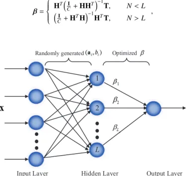
As shown in Fig. 1, ELM, which undertakes a three-layer structure, was originally proposed for the SLFNs and
140
was extended to the generalized SLFNs where the hidden layer needs not to be neuron alike. Different from other con-ventional approaches for training SLFNs, its hidden layer parameters (ai,bi) are generated randomly, so the learning problem can be reduced to that of estimating the optimal output weightβ[48].
Generally, ELM can be treated as a linear combination ofLactivation functions: fL(x)=
L ∑
i=1
βihi(x)=h(x)β, (1)
whereLdenotes the number of hidden nodes of ELM, andhi(x)=g(x,ai,bi). The above equation can be rewritten in matrix form as
Hβ=T, (2)
whereHis the hidden layer output matrix (randomized matrix):
H= h(x1) .. . h(xN) = h1(x1) · · · hL(x1) .. . . .. ... h1(xN) · · · hL(xN) , (3)
Tandβare the target matrix and output weight matrix of ELM:
T= tT1 .. . tT N and β= βT1 .. . βTL . (4)
Unlike some traditional machine learning approaches, ELM aims to reach the smallest training error as well as the smallest norm of the output weights, so its objective function can be mathematically represented as
min :LELM= 1 2∥β∥ 2 +1 2C N ∑ i=1 ξ2i s.t.,h(xi)β=ti−ξi,i=1, ...,N , (5)
whereξi=[ξ1,m, ..., ξi,m]is the training error vector of themoutput nodes with respect to the training samplexi,Cis
145
a regularization factor for strengthening the generalization performance. Then, based on the Karush-Kuhn-Tucker (KKT) theorem, we have
β= HT(I C+HH T)−1T, N<L (I C +H TH)−1HTT, N>L , (6)
whereIis the unit matrix.
Randomly generated Optimized
Input Layer Hidden Layer Output Layer
1
2
L
Figure 1: Basic Structure of ELM
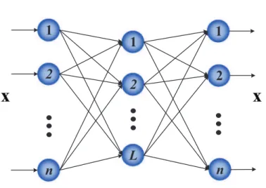
3.2. ELM Autoencoder
Autoencoder (AE) was proposed for using the encoded output to approximate the original input by minimizing the reconstruction errors, in which the output of an AE is set to be the same as the input, i.e.,T=X. AE has become a key stage in some deep architecture [49, 50, 51]. Different from the conventional AEs, in which back-propagation (BP) algorithm is usually implemented for training to obtain the identity function, Zhou et al. [26] proposed ELM-AE using ELM as the training algorithm for an AE, which is shown in Fig. 2. ELM-AE is an unsupervised neural network, in which its output is the same as the input. Thus, the input data will be reconstructed at the output layer by
L ∑
i=1
βig(xj,ai,bi)=xj,j=1, ...,N. (7)
The relationship between the input and the output can be mathematically represented in the matrix format as
Hβ=X. (8)
1) Compressed representation (representing features from a higher dimensional input data space to a lower dimen-sional feature space, as well as the number of the input samples is more than the number of hidden nodes):
β= (I C +H TH )−1 HTX. (9)
2) Sparse representation (representing features from a lower dimensional input data space to a higher dimensional feature space, as well as the number of the input samples is less than the number of hidden nodes):
β=HT ( I C+HH T )−1 X. (10)
3) Equal representation (representing features from an input data space dimension equals to feature space dimen-sion): β=H−1X. (11)
n
2
1
1
2
L
1
2
n
Figure 2: Structure Diagram of ELM-AE
4. MP-ELM-based Target’s Location Estimation
150
In this section, we will analyze the motivation of proposing a hierarchical ELM with probabilistic output for DFL, introduce the main framework of MP-ELM-based DFL, as well as detail the proposed MP-ELM.
4.1. Motivation of Hierarchical ELM with Probabilistic Output for DFL
Shallow machine learning approaches have been widely used for DFL, such as SVM, GP, and ELM, but these approaches are hard to filter the useful links from the wireless networks. Because most of the links in the monitoring
155
area are useless and redundant for target’s location estimation, and some of them even may degrade the localization accuracy. In addition, due to the uncertain wireless communication environment subject to the multi-path and fade phenomena, signal transmission in the wireless network is serious uncertain, this may also result in the reference points (RPs) associate with wireless signals with large noise and further exacerbate the corruption of the data. Usually, data preprocessing and manual feature extraction approaches are performed for improving the localization accuracy.
160
However, lots of time and effort are consumed in manually extracting useful information for the specific problems. In addition, the aforementioned strategies make the data preprocessing or feature extraction and machine learning modeling become two isolated independent processes without intrinsic connection between them, which will have negative effects on the localization accuracy. In order to tackle these issues, deep learning approaches have applied to DFL, and obtained satisfactory performance. However, conventional deep learning approaches suffer from the
165
Usually, DFL actually belongs to the regression problem of the machine learning field, in which the target’s location can be estimated by matching the created radio map. When deep learning approaches are implemented, DFL can be converted to the classification problem (the number of classes equals to the number of reference points). In the monitoring area deploying with wireless networks, most of the links are useless for target’s location estimation,
170
which means much redundant information exists in the links. Therefore, considering the uncertainty of DFL, the deterministic approach with solid decision boundary, such as SVM, may not obtain satisfactory performance. Because if the decision making of a deterministic approach is wrong, there will be a lot of error during the localization phase, which degrades the localization accuracy significantly. However, if the decision boundary can be soft, the localization error may be reduced. In addition, the target’s location only can be estimated presumably, not determined precisely,
175
thus probabilistic approach should have better performance than the deterministic way in DFL.
When dealing with classification problem, one of the advantages of ELM is that it can be directly used for both the binary classification and multiclass classification problems. For a given testing sample, the output node with the largest decision function value denotes the class label. For the given dataset{(xi,ti)}Ni=1⊂Rn×Rm, each class label is expanded into a label vector with lengthmin ELM. Assuming thatxibelongs to class one, so the corresponding label
180
vector isti=[1,0, ...,0 | {z }
m ].
Traditionally, for the classification problem with mclasses, the output function vector of ELM classifier for a samplexcan be written as f(x)=[f1(x), ...,fm(x)], so we can determine the class label of samplexby
label(x)=arg maxfi(x), i=1,2, ...,m . (12) The goal of a classifier with deterministic output is usually to minimize the Euclidean mean squared error (Emse):
Emse=E T−T˜ 2 , (13)
whereT˜ denotes the corresponding estimated value ofT.
However, it cannot guarantee the trained ELM classifier can find the optimal solution, even if the output weight is theoretically global optimal, due to the limited capability of the given network structure [52]. Therefore, once the samples are classified with wrong labels, the classification error will be accumulated gradually.
185
Assuming thatT˜ =E[T|X] is the least square estimation ofT, thus, theith component ofT˜ can be represented as ˜ti=E[ti|X]=
∑ ti∈{0,1}
tiPr (ti|X)=Pr (ti=1|X). (14) According to the probabilistic approach, we can obtain the probability of the samples belonging to the specific classes, thus this kind of soft classification can reduce the negative effects of classification error accumulation on ELM classifier.
Based on the above analysis, if (12) gives the wrong class label of samplex, the localization accuracy will be seriously degraded. However, if ELMs (including classic ELM and hierarchical ELMs) can output the probabilistic estimation, it may be more suitable in classification with uncertainty. According to [53, 54], the output of the multi-layer perceptron is actually the approximation of Bayes optimal discriminant function for classification problem. Let fq(x,w) represent the output of theqth output node of the multilayer perceptron,wq denotes the correspondingqth class. Based on the Bayesian theory, the discriminant function can be represented as
Pr(wq|x ) = Pr ( x|wq ) Pr(wq ) m ∑ i=1 Pr (x|wi) Pr (wi) =Pr ( x,wq ) Pr (x) , (15) where Pr(x|wq )
denotes the conditional probability, Pr(wq) denotes the corresponding priori probability, Pr (x) is the probability density function, respectively. It should note that the distribution of{xi,ti}is actually characterized by
190
Pr (x).
Then, we have the following relationship:
Assuming that the outputs of the multilayer perceptron are restricted in 0 and 1, where 1 indicates the sample belongs to the target class, and 0 indicates it belongs to other classes. So the sample error can be represented as
E(w)=∑ x [ fq(x,w)−tq ]2 =∑ x∈wq [ fq(x,w)−1 ]2 +∑ x<wq [ fq(x,w)−0 ]2 =z zq z 1 zq ∑ x∈wq [ fq(x,w)−1 ]2 +z−zq z 1 z−zq ∑ x<wq [ fq(x,w)−0 ]2 , (17)
wherezis the total sample number,zqis the number of samples belonging to the classq, respectively. The average error can be represented as
Eave(w)=lim z→∞ 1 zE(w) =Pr(wq) ∫ [ fq(x,w)−1 ]2 Pr(x|wq)dx+Pr(wi,q) ∫ fq(x,w)2Pr(x|wi,q)dx = ∫ fq2(x,w) Pr(x)dx−2 ∫ fq(x,w) Pr(x,wq)dx+ ∫ Pr(x,wq)dx = ∫ [ fq(x,w)−Pr(wq|x) ]2 Pr(x)dx+ ∫ Pr(wq|x) Pr(wi,q|x) Pr(x)dx . (18)
Accordingly, we can find that the second term of (18) is independent withw, so the multilayer perceptron is to minimize Esum(w)= ∑∫ [ fq(x,w)−Pr(wq|x) ]2 Pr(x)dx. (19)
Observed from the above analysis, in the limit of infinite samples, the output of the multilayer perceptron will approximate the true posterior probabilities in a least-square sense, so we have fq(x,w) ≈ Pr(wq|x). It should note that ELM with hierarchical structure is also a kind of multilayer perceptron [27], so its output also can reflect the
195
posteriori probabilities of different classes. Thus, theoretically, ELM with hierarchical structure with outputting the probabilistic estimation is reasonable.
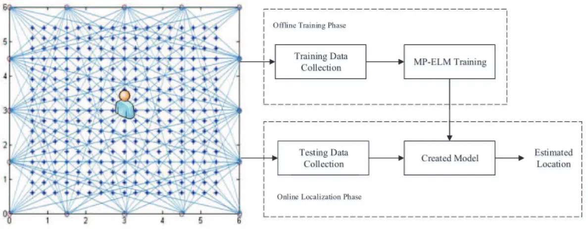
4.2. Main Framework of MP-ELM-based DFL
As shown in Fig. 3, the MP-ELM-based DFL involves two phases, i.e., the offline training phase and the online localization phase. During the offline training phase, RPs are used for data collection and MP-ELM training as the
200
samples. Each RP is associated with a number of links, and the corresponding links of all the RPs can be used for providing the training dataset. In the online localization phase, the target’s location can be estimated through the trained MP-ELM-based model.
Training Data
Collection MP-ELM Training
Created Model Estimated
Location Training Data
Collection MP-ELM Training
Offline Training Phase
Created Model Estimated
Location
Online Localization Phase
Testing Data Collection
Figure 3: Main Framework of the MP-ELM-based DFL
Assuming that there arelRPs, and each RP corresponds to jRSS values, so the input matrix of MP-ELM for DFL can be written as Input= ∆RS S1 1 ∆RS S 2 1 · · · ∆RS S j 1 ∆RS S12 ∆RS S22 · · · ∆RS S2j .. . ... . .. ... ∆RS S1 l ∆RS S 2 l · · · ∆RS S j l l×j . (20)
The calculated location coordinates of the target can be represented as
Coordinate= x1 y1 x2 y2 .. . ... xl yl l×2 , (21)
where, (xr,yr),r=1,2, . . . ,ldenotes the target’s location in DFL. 4.3. Multilayer Probability Extreme Learning Machine (MP-ELM)
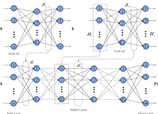
205
According to the analysis in Section 4.1, we will propose a novel hierarchical ELM with probabilistic output based on deep learning theory, named MP-ELM, for automatically extract useful information from the links, and implement-ing fast and accurate DFL. Fig. 4 illustrates the trainimplement-ing process of the proposed MP-ELM, which involves two phases in training its hierarchical architecture, i.e., the unsupervised feature representation phase and the supervised decision making phase. In the unsupervised feature representation phase, ELM-AE is implemented at each layer of MP-ELM for extracting the useful features layer by layer iteratively, that is to say, when the hidden layer parameters between the ith hidden layer and the (i−1)th hidden layer are trained using ELM-AE, the number of hidden nodes of theith hidden layer is identical to the number of hidden nodes of the corresponding ELM-AE. Before unsupervised feature learning, the raw data should be transformed into an ELM random feature space, which can help to exploit hidden information among training data. After that ak-layer unsupervised learning is performed to obtain the high-level useful features. The output of each hidden layer in MP-ELM can be represented mathematically as
Hi=g(βTi ·Hi−1), (22)
whereHidenotes the output matrix of theith hidden layer,Hi−1denotes the output matrix of the (i−1)th hidden layer,
andg(·) denotes the activation function of the hidden layers, respectively. Especially, wheni−1=0,H1becomes the
first hidden layer, andH0is actually the input layer of MP-ELM.
In the supervised decision making phase, an output layer with probabilistic estimation is implemented for final decision making. Considering the sigmoid function can convert an unbounded real number to a bounded real number
L1 Li+1 n Li 2 1 m 2 1 1 Lk 2 1 Li+1 2 Li 2 1 L1 2 1 2 1 1 2 1 2 n Input Layer Hidden Layers Output Layer 1 2 1 2 Li n 2 1 ELM-AE ELM-AE
Figure 4: Training Process of the Proposed MP-ELM
between 0 and 1, that is to say, when the input approaches+∞, the corresponding output will approach 1, and when the input approaches−∞, the corresponding output will approach 0, therefore, we construct the probabilistic output of MP-ELM based on the basic sigmoid function:
Pr(t=1|fq(x))=
1 1+exp(−fq(x))
. (23)
When the number of RPs equals to 2, MP-ELM-based DFL actually belongs to a binary classification problem, and when the number of RPs is larger than 2, it becomes a multiclass classification problem. For the binary classification problem, the sum of (23) always equals to 1, because the two outputs are opposite with each other. However, for the multiclass classification problem, the sum of (23) cannot guarantee to be 1, therefore, we normalize (23) by
∼ Pr(t=1|fq(x))= Pr(t=1|fq(x)) m ∑ i=1 Pr(t=1|fi(x)) . (24)
Then, the target’s location can be estimated as a weighted average of the locations of all the RPs: Location= m ∑ i=1 ∼ Pr(t=1|fi(x))·RPi. (25) 5. Performance Verification
In this section, we will evaluate the performance of the proposed MP-ELM-based DFL by comparing it with
210
classic ELM, ML-ELM, H-ELM, deep belief networks (DBN) [55], and deep Boltzmann machines (DBM) [56]. All the simulations are carried out in a workstation with an Inter Xeon CPU E5-2620 v4 @ 2.10GHz CPU and 32G RAM.
5.1. Experimental Settings
In the experiments, we build the wireless network using CC2530 ZigBee sensor nodes, which are based on the IEEE 802.15.4 standard and operate in the 2.4 GHz frequency band. RPs are set up uniformly in the monitoring area. In the performance evaluation processes, the data from RPs are used for training model and the data from testing points (TP) for validating. Each RP provides one training sample, and each TP provides one testing sample. The RSSs are sampled at the 5-min interval, the RSS values of all the RPs and TPs are collected 100 times, and the average values of these RPs and TPs consist of the training dataset and the testing dataset, respectively. Two different experiments are performed to evaluate the proposed MP-ELM, respectively for the indoor and the outdoor environments. In addition, we use the following localization accuracy as the evaluation criteria:
Acc= v t 1 z z ∑ i=1 (xi−x˜i)2+(yi−y˜i)2, (26) where (xi,yi) is the actual coordinates of the target, and ( ˜xi,y˜i) is the predicted coordinates of the target,zis the sample number.
215
5.2. User Specified Parameters in MP-ELM
For classic ELM, ML-ELM, H-ELM, and MP-ELM, there are two tuning parameters, i.e., the regularization factor C, and the number of hidden nodes L. In order to obtain satisfactory performance, both of the two user specified parameters should be chosen carefully and appropriately (sigmoid function as the activiation function). Fig. 5, Fig. 6, and Fig. 7 illustrate the relationship amongL,C, and localization accuracy of ML-ELM, H-ELM, and MP-ELM,
220
respectively, whereLis in the search range of{5,10, . . . ,200}, andCis in the search range of{2−20,2−15, . . . ,210}.
According to the three figures, we can find that ML-ELM has the fastest convergence speed, but its performance is not stable; H-ELM may be more stable, but its convergence speed is relatively slow; compared with H-ELM, the convergence speed of MP-ELM is relatively satisfactory, and it is more stable than ML-ELM.
0 25 50 75 100 125 150 175 200 2^(−20) 2^(−15) 2^(−10) 2^(−5) 2^(0) 2^(5) 2^(10) 0.5 1 1.5 2 2.5 3 3.5 C L Localization Accuracy (m)
0 25 50 75 100 125 150 175 200 2^(−20) 2^(−15) 2^(−10) 2^(−5) 2^(0) 2^(5) 2^(10) 0.5 1 1.5 2 2.5 3 3.5 C L Localization Accuracy (m)
Figure 6: Relationship amongL,C, and Localization Accuracy in H-ELM
0 25 50 75 100 125 150 175 200 2^(−20) 2^(−15) 2^(−10) 2^(−5) 2^(0) 2^(5) 2^(10) 0 0.5 1 1.5 2 2.5 3 C L Localization Accuracy (m)
Figure 7: Relationship amongL,C, and Localization Accuracy in MP-ELM
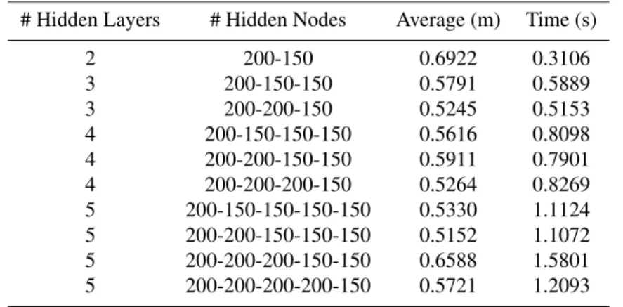
Table 1 lists the impacts of different numbers of hidden layers and hidden nodes on the performance of MP-ELM,
225
including the number of hidden layers, number of hidden nodes, average localization accuracy, and time consumption. According to Table 1, we can find that the speed of MP-ELM with two hidden layers is the fastest, but its average localization accuracy is not satisfactory. With the increase of hidden layer number, the average localization accuracies become better, but more hidden layer number makes MP-ELM time-consuming gradually. Thus, we choose the three-layer MP-ELM in the following experiments as a good trade-offbetween localization accuracy and time consumption,
230
whose number of hidden nodes in each hidden layer is 200, 200, and 150. In addition, in the following experiments, the hidden nodes number of ELM is set as 150; ML-ELM and H-ELM with three-layer structures are also set as 200, 200, and 150, respectively; for DBN and DBM, BP algorithm is used for training the hierarchical structures, and the initial learning rate is set as 0.1 with a decay rate 0.95 for each learning epoch.
Table 1: Comparison Results of MP-ELM with Different Numbers of Hidden Layers and Hidden Nodes
# Hidden Layers # Hidden Nodes Average (m) Time (s)
2 200-150 0.6922 0.3106 3 200-150-150 0.5791 0.5889 3 200-200-150 0.5245 0.5153 4 200-150-150-150 0.5616 0.8098 4 200-200-150-150 0.5911 0.7901 4 200-200-200-150 0.5264 0.8269 5 200-150-150-150-150 0.5330 1.1124 5 200-200-150-150-150 0.5152 1.1072 5 200-200-200-150-150 0.6588 1.5801 5 200-200-200-200-150 0.5721 1.2093
5.3. Evaluation in the Indoor Environment
235
In this section, we firstly evaluate the performance of the proposed MP-ELM-based DFL in the indoor environ-ment. As shown in Fig. 8, the indoor environment experiment was set up in a staffactivity room, and the monitoring area is a 6 m×6 m square, with 16 nodes placed along its boundary and the adjacent node distances of 1.5 m, and 0.3 m space between adjacent RPs. We randomly choose 10 TPs for performance evaluation.
Table 2 details the comparison results. Accordingly, we can find that MP-ELM obtains better localization
accura-240
cies in most of the TPs, as well as the average values, especially much better than ELM. In terms of time consumption, MP-ELM, ML-ELM, and H-ELM are hundreds of times faster than DBN and DBM, so it indicates that ELM with hierarchical structure is more suitable for dealing with big data problem than conventional deep learning approaches.
Figure 8: Data Collection in the Indoor Environment
Table 2: Comparison Results in the Indoor Environment (m)
Approach TP1 TP2 TP3 TP4 TP5 TP6 TP7 TP8 TP9 TP10 Average Time (s)
ELM 0.6579 0.6675 0.7189 0.7067 0.9857 0.7313 1.0267 0.3559 0.5887 0.7856 0.7225 0.0692 ML-ELM 0.5316 0.5087 0.6930 0.6516 0.8066 0.6241 0.7630 0.1341 0.4029 0.7392 0.5855 0.5925 H-ELM 0.4550 0.5910 0.5853 0.6259 0.8100 0.6058 0.7201 0.1931 0.3898 0.7085 0.5685 0.3587 DBN 0.5134 0.6035 0.5505 0.6570 0.7927 0.6133 0.7035 0.1690 0.3927 0.6630 0.5659 40.3997 DBM 0.5363 0.5291 0.5271 0.6613 0.8038 0.6513 0.7110 0.1555 0.4515 0.7277 0.5755 96.2299 MP-ELM 0.4579 0.5322 0.5630 0.6095 0.7890 0.6099 0.7179 0.1399 0.4201 0.6891 0.5529 0.5896
5.4. Evaluation in the Outdoor Environment
As shown in Fig. 9, the outdoor experiment was set up on the campus of the University of Science and Technology
245
Beijing. Similarly, the monitoring area is a 6 m×6 m square, with 16 nodes placed along its boundary and the adjacent node distances of 1.5 m, and 0.3 m space between adjacent RPs. 10 TPs are randomly chosen for evaluating the performance of MP-ELM.
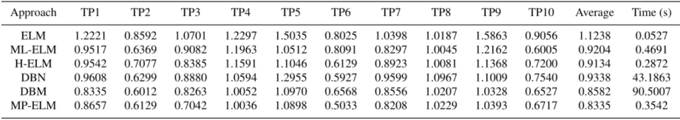
Table 3 demonstrates the detailed comparison results. According to Table 3, we can find that MP-ELM obtains better localization accuracies in most of the TPs, as well as the average values. In terms of time consumption,
MP-250
ELM, ML-ELM, and H-ELM are comparative, and still much faster than DBN and DBM.
Figure 9: Data Collection in the Outdoor Environment
Table 3: Comparison Results in the Outdoor Environment (m)
Approach TP1 TP2 TP3 TP4 TP5 TP6 TP7 TP8 TP9 TP10 Average Time (s)
ELM 1.2221 0.8592 1.0701 1.2297 1.5035 0.8025 1.0398 1.0187 1.5863 0.9056 1.1238 0.0527 ML-ELM 0.9517 0.6369 0.9082 1.1963 1.0512 0.8091 0.8297 1.0045 1.2162 0.6005 0.9204 0.4691 H-ELM 0.9542 0.7077 0.8385 1.1591 1.1046 0.6129 0.8923 1.0081 1.1368 0.7200 0.9134 0.2872 DBN 0.9608 0.6299 0.8880 1.0594 1.2955 0.5927 0.9599 1.0967 1.1009 0.7540 0.9338 43.1863 DBM 0.8335 0.6012 0.8263 1.0052 1.0970 0.6568 0.8556 1.0207 1.0328 0.6527 0.8582 90.5007 MP-ELM 0.8657 0.6129 0.7042 1.0036 1.0898 0.5033 0.8208 1.0229 1.0393 0.6717 0.8335 0.3542 6. Discussions
In some conventional deep learning approaches, the parameters of all the hidden layers need to be determined iteratively using BP algorithm, so the training process is time-consuming and cumbersome [57]. However, in the proposed MP-ELM, once the features of the previous hidden layer are extracted, the parameters of the current hidden
255
layer will be fixed, and need not to be fine-tuned. Therefore, the learning speed of MP-ELM is much faster than some conventional deep learning approaches. In the experiments, ELM is chosen as one of the comparison approaches. Unlike some deep learning approaches, there is no automatic feature extraction in ELM [58]. According to the experimental results, the localization accuracies of MP-ELM as well as other selected deep learning approaches are much better than ELM, which indicates that the feature extraction plays a central role in deep learning. In addition,
260
ELM is much faster than others due to its single-hidden-layer structure. However, ELM cannot function well in dealing with complex tasks, that is to say, ELM may be more suitable for simple tasks with big data. In those kinds of cases, ELM can obtain both satisfactory accuracy and little time consumption. For complex tasks with big data, MP-ELM is much faster than some conventional deep learning approaches, but with comparative accuracy.
Most of the links in the monitoring area are useless and redundant for target’s location estimation, that is to say,
265
classified with wrong labels, the classification error will accumulate gradually during the localization phase, which seriously degrades the localization accuracy. However, if we use MP-ELM, which is with probabilistic output, the decision boundary will be soft, we can obtain the probability of the samples belonging to the specific classes, so it can reduce the negative effects of classification error accumulation on the final localization accuracy. Thus, the proposed
270
MP-ELM has better performance than other deep learning approaches. In general, MP-ELM has three advantages: 1) it can reduce the chance of overfitting of the model by estimating the probability of samples’ attribution instead of fitting the samples; 2) it can reduce the error accumulation through the weighted average of the probability of the target’s location belonging to all the RPs; 3) it can enhance the reliability of the classifier through integrating hierarchical ELM with probabilistic approach. It should note that, to our best knowledge, the proposed MP-ELM is
275
the first hierarchical ELM with outputting the probabilistic estimation.
As mentioned above, one of the advantages of MP-ELM is the randomly generated hidden layer parameters, which makes it have very fast learning speed. Simultaneously, it also leads to the instability of MP-ELM. Because the randomization of the hidden layer parameters has significant impacts on the performance of ELM-AE. ELMs are actually sensitive to the range, and the change of the range may decrease the stability of MP-ELM. Unfortunately,
280
there is still no clear and theoretical criterion to guide the selection of the randomization range for different datasets. Usually, the randomization range is set as a specific interval, but different data have different distributions, so the results of MP-ELM may fluctuate in the specific range [59, 60, 61]. The theoretical analysis and experimental results indicate that MP-ELM is more suitable in dealing with large-scale and complex problems than some conventional deep learning approaches. Because the high time consumption of those deep learning approaches makes some short-term
285
problems meaningless, such as advertisement click ratio prediction and stock price prediction, etc. 7. Conclusions
In this paper, MP-ELM is proposed for automatically extracting useful information from the links, and imple-menting fast and accurate DFL. MP-ELM is stacked by ELM-AEs, and outputs the probabilistic estimation instead of fitting to data, so it has very fast learning speed as well as good generalization performance and robustness. Compared
290
with the conventional manual approaches for feature extraction in DFL, MP-ELM can automatically learning discrim-inative features form the links with less labor and time consumption. Compared with some conventional deep learning approaches, the learning speed of MP-ELM is much faster. In addition, different from the existing hierarchical ELMs, MP-ELM outputs the probabilistic estimation, but not the deterministic value, so it is more suitable in dealing with the complex tasks with uncertainty, such as DFL. Comprehensive experiments demonstrate the validity of the proposed
295
MP-ELM-based DFL. This paper only considers the localization problem with single target, so the future work will address the multi-target localization problem.
Acknowledgment
This work is supported in part by the National Key Research and Development Program of China under Grant 2017YFB1401203 and the National Natural Science Foundation of China under Grants 61673055, 61673056 and
300
61773056. References
[1] X.X. Lu, H. Zou, H.M. Zhou, L.H. Xie, G.B. Huang, Robust extreme learning machine with its application to indoor positioning, IEEE Trans. Cybern. 46 (1) (2016) 194-205.
[2] C. Medina, J.C. Segura, A.D. Torre, Ultrasound indoor positioning system based on a low-power wirless sensor network providing sub-305
centimeter accuracy, Sensors 13 (3) (2013) 3501-3526.
[3] J. Zhang, J. Sun, H.L. Wang, W.D. Xiao, L. Tan, Large-scale WiFi indoor localization via extreme learning machine, in: Proceedings of the 36th Chinese Control Conference, IEEE, 2017, pp. 4115-4120.
[4] W. Meng, W.D. Xiao, Energy-based acoustic source localization methods: a survey, Sensors 17 (2) (2017) 376-395.
[5] M. Youssef, M. Mah, A. Agrawala, A challenges: device-free passive localization for wireless environments, in: Proceedings of the 13th 310
Annual ACM International Conference on Mobile Computng and Networtking, Montreal, QC, Canada, 2007, pp. 222-229.
[6] J. Zhang, W.D. Xiao, S. Zhang, S.D. Huang, Device-free localization via an ectreme learning machine with paramterized geometrical feature extraction, Sensors 17 (4) (2017) 879-899.
[7] J. Wang, Q.H. Gao, M. Pan, Y.G. Fang, Device-free wireless sensing: challenges, opportunities, and applications, IEEE Netw. 32(2) (2018) 132-137.
315
[8] J. Wang, X. Zhang, Q.H. Gao, H. Yue, H.Y. Wang, Device-free wireless localization and activity recognition: a deep learning approach, IEEE Trans. Veh. Technol. 66 (7) (2017) 6258-6267.
[9] G.B. Huang, Q.Y. Zhu, C.K. Siew, Extreme learning machine: theory and applications, Neurocomptuing 70 (2006) 489-501.
[10] Y.J. Li, S. Zhang, Y.X. Yin, W.D. Xiao, J. Zhang, Parallel one-class extreme learning machine for imbalance learning based on Bayesian approach, J. Amb. Intel. Hum. Comp. 2018, DOI: 10.1007/s12652-018-0994-x.
320
[11] G.B. Huang, H. Zhou, X. Ding, R. Zhang, Extreme learning machine for regression and multiclass classification, IEEE Trans. Syst. Man Cybern. Part B Cybern. 42 (2) (2012) 513-529.
[12] Y.J. Li, S. Zhang, Y.X. Yin, J. Zhang, W.D. Xiao, A soft sensing scheme of gas utilization prediction for blast furnace via improved extreme learning machine, Neural Process. Lett. 2018, DOI: 10.1007/s11063-018-9888-3.
[13] J. Zhang, Y.F. Lu, B.Q. Zhang, W.D. Xiao, Device-free localization using empirical wavelet transform-based extreme learning machine, in: 325
Proceedings of the 30th Chinese Control and Decision Conference, IEEE, 2018, pp. 2585-2590.
[14] R.Z. Song, W.D. Xiao, Q.L. Wei, C.Y. Sun, Neural-network-based approach to finite-time optimal control for a class of unknown nonlinear systems, Soft Comput. 18 (2014) 1645-1653.
[15] J. Zhang, Y.F. Xu, J.Q. Xue, W.D. Xiao, Real-time prediction of solar radiation based on online sequentual extreme learning machine, in: Proceedings of the 13th IEEE Conference on Indutrial Electronics and Applications, IEEE, 2018, pp. 53-57.
330
[16] Y.J. Li, S. Zhang, Y.X. Yin, W.D. Xiao, J. Zhang, A novel online sequential extreme learning machine for gas utilization ratio prediction in blast furnaces, Sensors 17 (8) (2017) 1847-1870.
[17] M.M. Liu, B. Liu, C. Zhang, Semi-supervised low rank kernel learning algorithm via extreme learning machine, Int. J. Mach. Learn. Cybern. 8 (3) (2017) 1039-1052.
[18] S.F. Ding, N. Zhang, J. Zhang, Unsupervised extreme learning machine with represnetational features, Int. J. Mach. Learn. Cybern. 8 (2) 335
(2017) 587-595.
[19] J.H. Zhai, S.F. Zhang, C.X. Wang, The classification of imlalanced large data sets based on MapReduce and ensemble of ELM classifiers, Int. J. Mach. Learn. Cybern. 8 (3) (2017) 1009-1017.
[20] W.D. Xiao, J. Zhang, Y.J. Li, S. Zhang, W.D. Yang, Class-specific cost regulation extreme learning machine for imbalanced classification, Neurocomptuing, 261 (2017) 70-82.
340
[21] W.T. Mao, J.W. Wang, Z.A. Xue, An ELM-based model with sparse-weighting strategy for sequential data imbalance problem, Int. J. Mach. Learn. Cybern. 8 (4) (2017) 1333-1345.
[22] J. Wang, L. Zhang, J.J. Cao, D. Han, NBWELM: naive Bayesian based weighted extreme learning machine, Int. J. Mach. Learn. Cybern. 9 (1) (2018) 21-35.
[23] J. Zhang, W.D. Xiao, Y.J. Li, S. Zhang, Residual compensation extreme learning machine for regression, Neurocomptuing, 311 (2018) 345
126-136.
[24] W.C. Yu, F.Z. Zhuang, Q. He, Z.Z. Shi, Learning deep representations via extreme learning machines, Neurocomptuing, 149 (2015) 308-315. [25] L.L.C. Kasun, H.M. Zhou, G.B. Huang, C.M. Vong, Representational learning with ELMs for big data, IEEE Intell. Syst. 28(6) (2013) 31-34. [26] H.M. Zhou, G.B. Huang, Z.P. Lin, H. Wang, Y.C. Soh, Stacked extreme learning machines, IEEE Trans. Cybern. 45 (9) (2015) 2013-2025. [27] J.X. Tang, C.W. Deng, G.B. Huang, Extreme learning machine for multilayer perceptron, IEEE Trans. Neural Netw. Lear. Syst. 27 (4) (2016) 350
809-821.
[28] N. Zhang, S.F. Ding, Z.Z. Shi, Denoising Laplacian multi-layer extreme learning machine, Neurocomptuing, 171 (2016) 1066-1074. [29] K. Sun, J. Zhang, C. Zhang, J. Hu, Generalized extreme learning machine autoencoder and a new deep neural network, Neurocomptuing, 230
(2017) 374-381.
[30] C.M. Wong, C.M. Vong, P.K. Wong, J.W. Cao, Kernel-based multilayer extreme learning machines for representation learning, IEEE Trans. 355
Neural Netw. Lear. Syst. 29 (3) (2018) 757-762.
[31] I. Sabek, M. Youssef, A.V. Vasilakos, ACE: an accurate and efficient multi-entity device-free WLAN localization system, IEEE Trans. Mob. Comput. 12 (2013) 1321-1334.
[32] H. Aly, M. Youssef, New insight into WiFi-based device-free localization, in: Proceedings of the 2013 ACM Conference on Pervasive and Ubiquitous Computng (UbiComp13), New York, NY, USA, 2013, pp. 541-548.
360
[33] Y.Y. Chiang, W.H. Hsu, S.C. Yeh, J.S. Wu, Fuzzy support vector machines for device-free localization, in: Proceedings of the IEEE Interna-tional and Measurement Technology Conference, IEEE, 2012, pp. 1-4.
[34] B. Song, H.L. Wang, W.D. Xiao, S.D. Huang, L. Shi, Gaussian process model enabled particle filter for device-free localization, in: Proceed-ings of the 20th International Conference on Information Fusion, IEEE, 2017, pp. 1-6.
[35] J. Wilson, N. Patwari, Radio tomographic imaging with wireless networks, IEEE Trans. Mob. Comput. 9 (5) (2010) 621-632. 365
[36] J. Wilson, N. Patwari, See through walls: motion tracking using variance-based radio tomography networks, IEEE Trans. Mob. Comput. 10 (2011) 612-621.
[37] Q. Lei, H.J. Zhang, H. Sun, L.L. Tang, A new elliptical model for device-free localization, Sensors 16 (4) (2016) 577-588.
[38] J. Wilson, N. Patwari, A fade level skew-Lapace signal strength model for device-free localization with wireless networks, IEEE Trans. Mob. Comput. 11 (2012) 947-958.
370
[39] A. Banerjee, M. Maheshwari, N. Patwari, S.K. Kasera, Detecting receiver attacks in VRTI-based device free localization, in: Proceedings of the 2012 IEEE International Symposium on a World of Wireless, Mobile and Multimedia, IEEE, 2012, pp. 1-6.
[40] Y. Zhao, N. Patwari, Robust estimators for varianced-based device-free localization and tracking, IEEE Trans. Mob. Comput. 14 (10) (2015) 2116-2129.
[41] J. Wang, Q. Gao, X. Zhang, H. Wang, Device-free localization with wireless networks based on compressive sensing, IET Commun. 6 (15) 375
(2012) 2395-2403.
[42] J. Wang, Q.H. Gao, H.Y. Wang, Y. Yu, M.L. Jin, Time-of-fight-based radio tomography for device free localization, IEEE Trans. Wirel. Commun. 5 (12) (2013) 2355-2365.
[43] J. Wang, X. Chen, D. Fang, D. Wu, Z. Yang, T. Xing, Transfering compressive-sensing-based device-free localization across target diversity, IEEE Trans. Ind. Electron. 62 (2015) 2397-2409.
380
[44] M.C.R. Talampas, K.S. Low, An enhanced geometric filter algorithm with channel diversity for device-free localization, IEEE Trans. Instrum. Meas. 65 (2016) 378-387.
[45] H. Wang, D.Q. Zhang, K. Niu, Q. Lv, Y.H. Liu, D. Wu, R.Y. Gao, B. Xie, A multicarrier Fresnel penetration model based device-free localization system leveraging commodity Wi-Fi cards, arXiv:1707.07514.
[46] J. Wang, Q. Gao, P. Cheng, L. Wu, K. Xin, H.Y. Wang, Lightweight roubust device-free localization in wireless networks, IEEE Trans. Ind. 385
Electron. 61 (2014) 5681-5689.
[47] S. Savazzi, M. Nicoli, F. Carminati, M. Riva, A Bayesian approach to device-free localization: modeling and experimental assessment, IEEE J. Sel. Top. Signal Process. 8 (2014) 16-29.
[48] G.B. Huang, An insight into extreme learning machines: random neurons, random features and kernels, Cogn. Comput. 6 (3) (2014) 376-390. [49] G. Hinton, S. Osindero, Y.W. Teh, A fast learning algorithm for deep belief nets, Neural Comput. 18 (7) (2006) 1527-1554.
390
[50] G. Hinton, R. Salakhutdinov, Reducing the dimensionality of data with neural networks, Science 313 (5786) (2006) 504-507. [51] Y. LeCun, Y. Bengio, G. Hinton, Deep learning, Nature 521 (5) (2015) 436-444.
[52] E.A. Wan, Neural network calssification: a Bayesian interpretation, IEEE Trans. Neural Netw. 1 (4) (1990) 296-298.
[53] D.W. Ruck, S.K. Rogers, M. Kabrisky, M.E. Oxley, B.W. Suter, The multiulayer perceptron as an approximation to a Bayes optimal discrim-inant function, IEEE Trans. Neural Netw. 1 (4) (1990) 303-305.
395
[54] H.L. Yu, C.Y. Sun, W.K. Yang, X.B. Yang, X. Zuo, AL-ELM: one uncertainty-based active learning algorithm using extreme learning machine, Neurocomptuing, 166 (2015) 140-150.
[55] G. Hinton, S. Osindero, Y. Teh, A fast learning algorithm for deep belief nets, Neural Comput. 18 (7) (2006) 1527-1554.
[56] R. Salakhutdinov, G. Hinton, Deep Boltzmann machines, in: Proceedings of the 12th International Conference on Artificial Intelligence Statistics, 2009, pp. 448-455.
400
[57] X.Z. Wang, T.L. Zhang, R. Wang, Non-iterative deep learning: incorporating restricted Boltzmann machine into multilayer random weight nerual networks, IEEE Trans. Syst. Man Cybern. Syst. 2017, DOI: 10.1109/TSMC.2017.2701419.
[58] X.M. Zhao, W.P. Cao, H.Y. Zhu, Z. Ming, R.A.R. Ashfaq, An intial study on the rank of input matrix for extreme learning machine, Int. J. Mach. Learn. Cybern. 9 (5) (2018) 867-879.
[59] X.Z. Wang, R. Wang, C. Xu, Discovering the relationship between generalization and uncertainty by incorporaing complexity of classification, 405
IEEE Trans. Cybern. 48 (2) (2018) 703-715.
[60] X. Liu, S.B. Liu, J. Fang, Z.B. Xu, Is extreme learning machine feasible? A theoretical assessment (part I), IEEE Trans. Neural Netw. Lear. Syst. 26 (1) (2015) 7-20.
[61] S.B. Liu, X. Liu, J. Fang, Z.B. Xu, Is extreme learning machine feasible? A theoretical assessment (part II), IEEE Trans. Neural Netw. Lear. Syst. 26 (1) (2015) 21-34.