A Thesis by
ASHWATH KUMAR KRISHNA REDDY
Submitted to the Office of Graduate Studies of Texas A&M University
in partial fulfillment of the requirements for the degree of MASTER OF SCIENCE
August 2010
A Thesis by
ASHWATH KUMAR KRISHNA REDDY
Submitted to the Office of Graduate Studies of Texas A&M University
in partial fulfillment of the requirements for the degree of MASTER OF SCIENCE
Approved by:
Chair of Committee, Annapareddy Narasimha Reddy Committee Members, Riccardo Bettati
Srinivas Shakkottai Head of Department, C. Georghiades
August 2010
ABSTRACT
Detecting Networks Employing Algorithmically Generated Domain Names. (August 2010)
Ashwath Kumar Krishna Reddy, B.Tech, National Institute of Technology Karnataka, India
Chair of Advisory Committee: Dr. Annapareddy Narasimha Reddy
Recent Botnets such as Conficker, Kraken and Torpig have used DNS based “domain fluxing” for command-and-control, where each Bot queries for existence of a series of domain names and the owner has to register only one such domain name. In this report, we develop a methodology to detect such “domain fluxes” in DNS traffic by looking for patterns inherent to domain names that are generated algorithmically, in contrast to those generated by humans. In particular, we look at distribution of alphanumeric characters as well as bigrams in all domains that are mapped to the same set of IP-addresses. We present and compare the performance of several distance metrics, including KL-distance and Edit distance. We train by using a good data set of domains obtained via a crawl of domains mapped to all IPv4 address space and modeling bad data sets based on behaviors seen so far and expected. We also apply our methodology to packet traces collected at two Tier-1 ISPs and show we can automatically detect domain fluxing as used by Conficker botnet with minimal false positives. We are also able to detect new botnets and other malicious networks using our method.
ACKNOWLEDGMENTS
My sincere thanks to my advisor Dr.A.L.Narasimha Reddy for being very patient during my course of research and for being an extraordinary mentor, and believing in me. His methods of intuitive thinking, research methodology and outlook on life will be something I will treasure and learn from in the years to come. I would also like to thank Dr. Srinivas Shakkotai and Dr. Ricardo Bettati for being part of my committee.
I would like to thank Sandeep Yadav (Phd student under the guidance of Dr. Annapareddy Narasimha Reddy) who was my companion through my course of study. This work would not have been possible without his help in developing, the right usage of the detection metrics.
I would like to extend a warm thank you to my parents for their constant love, support and encouragement. Last, but not the least my special thanks to my lovely fiance for making my hectic graduate school life memorable and fun-filled.
TABLE OF CONTENTS
CHAPTER Page
I INTRODUCTION . . . 1
II RELATED WORK . . . 9
III DETECTION METRICS. . . 12
3.1 Motivation . . . 12
3.2 Metrics for anomaly detection . . . 15
3.2.1 Measuring K-L divergence with unigrams . . . 16
3.2.2 Measuring K-L divergence with bigrams . . . 17
3.2.3 Edit distance . . . 18
IV GROUPING DOMAIN NAMES . . . 20
4.1 Per-domain analysis . . . 20
4.2 Per-IP analysis . . . 20
4.3 Component analysis . . . 21
4.3.1 Filter F1 . . . 22
4.3.2 Connected component extraction . . . 22
4.3.3 Component separation . . . 24
4.3.4 Feature extraction . . . 28
4.3.5 Training and prediction . . . 28
V RESULTS . . . 30
5.1 Per-domain analysis . . . 30
5.1.1 Data set . . . 30
5.1.2 K-L divergence with unigram distribution . . . 31
5.1.3 K-L divergence with bigram distribution . . . 31
5.1.4 Edit distance of sub-domains . . . 32
5.2 Per-IP analysis . . . 33
5.2.1 Data set . . . 33
5.2.2 Results . . . 34
5.3 Component analysis results . . . 35
5.3.1 Methodology . . . 35
5.3.2 Results . . . 36
CHAPTER Page
6.1 Usefulness of component analysis . . . 46
6.2 Complexity of various measures . . . 48
VII CONCLUSION . . . 51
LIST OF TABLES
TABLE Page
I Different types of classes . . . 36 II Behavior of the type of component . . . 37 III Detailed results for each class . . . 38 IV Summary of interesting networks discovered through component
analysis . . . 41 V Domain names used by bots . . . 43 VI Computational complexity . . . 49
LIST OF FIGURES
FIGURE Page
1 Probability distribution of alphanumeric characters for
malicious/non-malicious datasets. . . 14
2 Probability distribution of alphanumeric characters for malicious datasets.. . . 15
3 Probability distribution of bigram indices for legitimate and ma-licious datasets. . . 17
4 Connected component analysis flowchart.. . . 21
5 Different component classes. . . 24
6 ROC curve : Edit distance (Per-domain). . . 32
7 ROC curve : K-L metric with bigram distribution (Per-IP). . . 33
8 Conficker botnet analysis for various groups. . . 47
CHAPTER I
INTRODUCTION
Botnets are posing a major security threat to most of the computers over the internet. They are the major source of attacks like distributed denial of service attacks, phish-ing, identity theft and spam. The botnets use IRC (Internet Relay Chat), HTTP and Peer to Peer protocols as a command and control channel to infect the bots. The botnets operate in a centralized manner where there is a centralized machine which controls all the bots (zombie machines). The centralized machine is called the Command and Control (C&C) server which controls the zombie infected machines called the bots. These C&C servers use custom protocols to communicate and convey information to the bots. The bots contact the servers on a regular basis to receive updates from the C&C servers, by this all the bots would perform the same operation at a given time. These C&C servers use bots to launch a coordinated group attack of spreading malware, sending spam or launching a denial of service attack. The botnets frequently change their signatures and the way they contact the C&C servers. The signature of a C&C protocol would correspond to the interval of contact between the C&C server and the bots, the pattern in which the bots would contact different C&C servers etc. Most of the packets involved in the communication are encrypted and a few bits maybe inserted in the middle of the fields to mislead the detection systems. Recently botnets have started using the Peer to Peer model for communication where every machine acts as a controller; it becomes very difficult for the detector to track
the activities of the botnet.
Now a days the C&C protocol runs over HTTP to evade detection. HTTP is a very common protocol which is not blocked by most of the machines on the internet. The detection with other protocols would be easier compared to HTTP. The bots would contact the C&C server by querying a domain name. This domain name has to be changed with time else the domain name would be blacklisted by the DNS blacklists and the bots would not be able to establish the C&C channel. To overcome this problem of blacklisting, the bot groups would need to change their domain names on a regular basis. Most of the general/regularly used domain names would very likely be registered. It is also very likely that most of the regular english dictionary names would already be registered. To overcome these problems the C&C servers not being able to register standard english dictionary domain names, they resort to generating random domain names. The C&C servers generate domain names using a random name generator and they register a few of these randomly generated domain names. The bot and the C&C server would generate the same domain names since they would have the same domain generation algorithm with the same seed. The bot would query all the domain names generated by the random name generator and would successfully contact the C&C server on the domain name/names registered by the C&C server.
Recent botnets such as Conficker, Kraken and Torpig have brought in vogue a new method for botnet operators to control their bots: DNS “domain fluxing”. In this method, each bot algorithmically generates a large set of domain names and queries each of them until one of them is resolved and then the bot contacts the corresponding IP-address obtained that is typically used to host the command-and-control (C&C) server. Besides for command-and-command-and-control, spammers also routinely generate random domain names in order to avoid detection. For instance, spammers advertise randomly generated domain names in their spam emails to avoid detection
by regular expression based domain blacklists that maintain signatures for recently ‘spamvertised’ domain names. This is done to evade domain blacklists i.e., blacklists of bad domain names that are hosting malware, spyware, etc.
This is in contrast to the more common practice of DNS “IP fast-fluxing” where one domain name is mapped to a changing set of IP-addresses [1]. If a combination of the two happen, then this would be even more difficult to detect. To detect Conficker’s domain generation algorithm, scientists had to reverse engineer the domain generation algorithm, something definitely not scalable for similar attacks in the future. We design techniques to show how DNS domain fast fluxing can be automatically detected without having to reverse engineer the domain generation algorithm itself.
The botnets that have used random domain name generation vary widely in the random word generation algorithm as well as the way it is seeded. For instance, Conficker-A [2] bots generate 250 domains every three hours while using the current date and time at UTC as the seed, which in turn is obtained by sending empty HTTP GET queries to a few legitimate sites such as google.com, baidu.com, answers.com,
etc. This way, all bots would generate the same domain names every day. In order to make it harder for a security vendor to pre-register the domain names, the next version, Conficker-C [3] increased the number of randomly generated domain names per bot to 50K. Torpig [4], [5] bots employ an interesting trick where the seed for the random string generator is based on one of the most popular trending topics in Twitter. Kraken employs a much more sophisticated random word generator and con-structs English-language alike words with properly matched vowels and consonants. Moreover, the randomly generated word is combined with a suffix chosen randomly from a pool of common English nouns, verbs, adjective and adverb suffixes, such as -able, -dom, -hood, -ment, -ship, or -ly. Storm botnet uses english words with random suffices as domain names. For example Conficker A uses a domain name generator
250 domains every 3 hours. Their domain names are 5-11 characters long and the randomization function they use is the date. Conficker B generates 200 domain names every 2 hours and a different seed used for the randomization function. The set of the 200 domain names are different. Conficker C generates 50000 domain names, so the generation of domain names gets more complex.
From the point of view of botnet owner, the economics work out quite well. They only have to register one or a few domains out of the several domains that each bot would query every day. Whereas, security vendors would have to pre-register
all the domains that a bot queries every day, even before the botnet owner registers them. In all the cases above, the security vendors had to reverse engineer the bot executable to derive the exact algorithm being used for generating domain names. In some cases, their algorithm would predict domains successfully until the botnet owner would patch all his bots with a repurposed executable with a different domain generation algorithm [4].
We argue that reverse engineering of botnet executables is resource- and time-intensive and precious time may be lost before the domain generation algorithm is cracked and consequently before such domain name queries generated by bots are detected. In this regards, we raise the following question: can we detect algorith-mically generated domain names while monitoring DNS traffic even when a reverse engineered domain generation algorithm may not be available?
Hence, we propose a methodology that analyzes DNS traffic to detect if and
when domain names are being generated algorithmically as a line of first defense. In this regards, our proposed methodology can point to the presence of bots within a network and the network administrator can disconnect bots from their C&C server by filtering out DNS queries to such algorithmically generated domain names.
do not use well formed and pronounceable language words since the likelihood that such a word is already registered at a domain registrar is very high; which could be self-defeating as the botnet owner would then not be able to control his bots. In turn this means that such algorithmically generated domain names can be expected to exhibit characteristics vastly different from legitimate domain names. Hence, we develop metrics using techniques from signal detection theory and statistical learning which can detect algorithmically generated domain names that may be generated via a myriad of techniques:
1. Those generated via pseudo-random string generation algorithms as well as
2. Dictionary-based generators, for instance the one used by Kraken[6], [7], [8] as well as a publicly available tool, Kwyjibo [9] which can generate words that are pronounceable yet not in the english dictionary.
Our method of detection comprises of two parts. First, we propose several ways to group together DNS queries:
1. Either by the Top Level Domain (TLD) they all correspond to or;
2. The IP-address that they are mapped to or;
3. the connected component that they belong to, as determined via connected component analysis of the IP-domain bipartite graph.
Second, for each such group, we compute metrics that characterize the distri-bution of the alphanumeric characters or bigrams (two consecutive alphanumeric characters) within the set of domain names.
Our contribution is a methodology for detecting algorithmically generated strings as used in URLs for the purpose of either command-and-control of Botnets or for
hosting spammed products, e.g. sites which peddle products that are advertised via spam. Our methodology is based on the observation that to generate strings algorith-mically, current botnets use simple pseudo-random generators which may not preserve the distribution of alphabets or bigrams (two consecutive alphabets) as usually occur in legitimate domain name strings. In this regards, we propose several metrics to classify a set of domain names as legitimate or malicious - by that are based on the distribution of alphanumeric characters between legitimate domains and malicious ones. In particular, we propose metrics that are based on the
1. Information entropy of the distribution of alphanumerics (unigrams and bi-grams) within a group of domains;
2. Edit-distance which measures the number of character changes needed to con-vert one domain name to another.
We apply our methodology to a variety of data sets. First, we obtain a set of legitimate domain names via reverse DNS crawl of the entire IPv4 address space. Next, we obtain a set of malicious domain names as generated by Conficker, Kraken and Torpig as well as model a much more sophisticated domain name generation algo-rithm: Kwyjibo [9]. Finally, we apply our methodology to one day of network traffic from two Tier-1 ISPs from Asia and Brazil and show how we can detect Conficker as well as a botnet hitherto unknown, which we call Mjuyh (details in Chapter V).
Our extensive experiments allow us to characterize the effectiveness of each met-ric in detecting algorithmically generated domain names in different attack scenarios. We model different attack intensities as number of domain names that an algorithm generates. For instance, in the extreme scenario that a botnet generates 50 domains mapped to the same TLD, we show that KL-divergence over unigrams achieves 100% detection accuracy albeit at 15% false positive rate (legitimate domain groups
clas-sified as algorithmic). We show how our detection improves significantly with much lower false positives as the number of words generated per TLD increases, e.g., when 200 domains are generated per TLD, then Edit distance achieves 100% detection accuracy with 8% false positives and when 500 domains are generated per TLD.
Finally, our methodology of grouping together domains via connected compo-nents allows us to detect not only “domain fluxing” but also if it was used in combi-nation with “IP fluxing”. Moreover, computing the metrics over components yields better and faster detection than other grouping methods. Intuitively, even if botnets were to generate random words and combine them with multiple TLDs in order to spread the domain names thus generated (potentially to evade detection), as long as they map these domains such that at least one IP-address is shared in common, then they are revealing a group structure that can be exploited by our methodology for quick detection. We show that per-component analysis detects 26.32% more IP addresses than using IP analysis and 16.13% more hostnames than using per-domain analysis when we applied our methodology to detect Conficker in a Tier-1 ISP trace.
Finally, we note that detecting malicious activity in a network by analyzing DNS traffic serves the following additional benefits:
1. We need to analyze a much smaller amount of traffic, for example, for the ISP trace we analyze in our work here, the DNS traffic volume is 0.35% smaller, 237 MB compared to 66 GB for the entire trace;
2. Works even if the rest of the traffic that is sent by a bot is encrypted, which frequently occurs since after determining the C&C server to communicate with, the bot may thereafter use HTTPS for further communication.
detection methodology and introduce the metrics we have developed. In Chapter IV we present our connected component algorithm. In Chapter V we present results with the component analysis. In Chapter II we compare our work against related literature and in Chapter VII we conclude.
The work has been done in collaboration with Sandeep Yadav (Phd student working under the guidance of Dr. A.L.Narasimha Reddy, Texas A & M University). The code and the Per-IP, Per-Domain analysis for the metrics as shown in Chapter III have been developed by Sandeep. Extraction and analysis of components and application of these metrics on the components to detect other malicious components in the ISP trace has been the major part of my work. This work has been submitted to the Internet Measurement Conference, 2010 [10] and is in review.
CHAPTER II
RELATED WORK
Characteristics, such as IP addresses, whois records and lexical features of phishing and non-phishing URLs have been analyzed by McGrath and Gupta [11]. They observed that the different URLs exhibited different alphabet distributions. Our work builds on this earlier work and develops techniques for identifying domains employing algorithmically generated names, potentially for “domain fluxing”. Ma, et al [12], employ statistical learning techniques based on lexical features (length of domain names, host names, number of dots in the URL etc.) and other features of URLs to automatically determine if a URL is malicious, i.e., used for phishing or advertising spam. While they classify each URL independently, our work is focused on classifying a group of URLs as algorithmically generated or not, solely by making use of the set of alphanumeric characters used. In addition, we experimentally compare against their lexical features in Chapter V and show that our alphanumeric distribution based features can detect algorithmically generated domain names with lower false positives than lexical features. Overall, we consider our work as complimentary and synergistic to the approach in [12]. Our work employs similar techniques in combination with an analysis of DNS traffic to determine the malicious nature of domains.They [12] have multiple lexical features like the number of dots in the URL, the length of the domain name etc. Here the training database needs to be very good for an accurate prediction.
With reference to the practice of “IP fast fluxing”,e.g., where the botnet owner constantly keeps changing the IP-addresses mapped to a C&C server, [1] implements
a detection mechanism based on passive DNS traffic analysis. In this work IP fast fluxing is easily detected but the domain fluxing problem is not directly addressed. So not all the botnet groups can be detected by this model. In our work, we present a methodology to detect cases where botnet owners may use a combination of both domain fluxing with IP fluxing, by having bots query a series of domain names and at the same time map a few of those domain names to an evolving set of IP-addresses. Also earlier papers [13], [14] have analyzed the inner-working of IP fast flux networks for hiding spam and scam infrastructure. Here the bots in the same botnet exhibit similar characteristics in terms of C&C communication and similar malicious activi-ties. This assumption also holds for sub-botnets where a big botnet performs many different malicious activities. With regards to botnet detection, [15], [16] perform correlation of network activity in time and space at campus network edges. Our work does not require to consider the complete network traffic as these authors and we consider only the DNS traffic. Thereby we get a considerable reduction in both the length of the trace to be analyzed and the complexity of the operation. Xie et al in [17] focus on detecting spamming botnets by developing regular expression based signatures from a dataset of spam URLs. This work is similar to our work, here the model would be trained to detect a particular signature. In this work, a training for each particular signature would be required to detect a given signature whereas our work is generic.
We find that graph analysis of IP addresses and domain names embedded in DNS queries and replies reveal interesting macro relationships between different entities and enable identification of bot networks (Conficker) that seemed to span many domains and TLDs. With reference to graph based analysis, [18] utilizes rapid changes in user-user graphs structure to detect botnet accounts. They extract the relationships and correlations among botnet activities by constructing large user-user graphs and
then looking for strongly connected components.
Statistical and learning techniques have been employed by various studies for prediction [19], [20], [21]. Spam filtering [19] is discussed using adaptive statistical data compression models. New features in the payload are extracted [20] feature clustering for text classification. The automated abuse of chat programs [21] by the chat bots are tackled. All the statistical learning techniques [19], [20], [21] would detect the bot network it has been trained to detect. These techniques would require additional training to detect any new bot network. However our model would not require any additional training for a new bot network. We employed results from detection theory in designing our strategies for classification [22], [23].
Several studies have looked at understanding and reverse-engineering the inner workings of botnets [6], [7], [8], [24], [4], [25], [26]. Botlab has carried out an extensive analysis of several bot networks through active participation [27] and provided us with many example datasets for malicious domains. The authors [27] analyze spam-based botnets where they collect the spam based data from all the botnets and they later use this data to predict many botnets like Storm, Conficker, Kraken, Mega-D.
CHAPTER III
DETECTION METRICS
In this Chapter, we present our detection methodology that is based on computing the distribution of alphanumeric characters for groups of domains. First, we moti-vate our metrics by showing how algorithmically generated domain names differ from legitimate ones in terms of distribution of alphanumeric characters. Next, we present our two metrics, namely Kullback-Leibler (KL) distance and Edit distance. Finally, in Section IV we present the methodology to group domain names.
3.1 Motivation
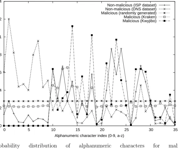
Our detection methodology is based on the observation that algorithmically gener-ated domains differ significantly from legitimate (human) genergener-ated ones in terms of the distribution of alphanumeric characters. Figure 1 shows the distribution of al-phanumeric characters, defined as the set of English alphabets (a-z) and digits (0-9) for the legitimate domains and the Figure 2 shows the distribution for the malicious domains1.
The explanation of the data sets used is given below:
1. Non-malicious ISP Dataset: We use network traffic trace collected from across 100+ router links at a Tier-1 ISP in Asia. The trace is one day long and provides details of DNS requests and corresponding replies. There are about 270,000 DNS name server replies.
1Even though domain names may contain characters such as ‘-’, we currently limit
2. Non-malicious DNS Dataset: We performed a reverse DNS crawl of the entire IPv4 address space and then filtered out the legitimate domain names to obtain a list of domain names and their corresponding IP-addresses. We further divided this data set in to several parts, each comprising of domains which had 500, 200, 100 and 50 sub-domains.
3. Malicious datasets: We obtained the list of domain names that were known to have been generated by recent Botnets: Conficker [2], [3], Torpig [4] and Kraken [6], [7]. As described earlier in the Introduction, Kraken exhibits the most sophisticated domain generator by carefully matching the frequency of occurrence of vowels and consonants as well as concatenating the resulting word with common suffixes in the end such as -able, -dom, etc.
4. Kwyjibo: We model a much more sophisticated algorithmic domain name gen-eration algorithm by using a publicly available tool, Kwyjibo [9] which generates domain names that are pronounceable yet not in the English language dictio-nary and hence much more likely to be available for registration at a domain registrar. The algorithm uses a syllable generator, where they first learn the frequency of one syllable following another in words in English dictionary and then automatically generate pronounceable words by modeling it as a Markov process.
Later we derive the following points:
1. First, note that both the non-malicious data sets exhibit a non-uniform fre-quency distribution, e.g., letters ‘m’ and ‘o’ appear most frequently in the non-malicious ISP data set whereas the letter ‘s’ appears most frequently in the non-malicious DNS data set.
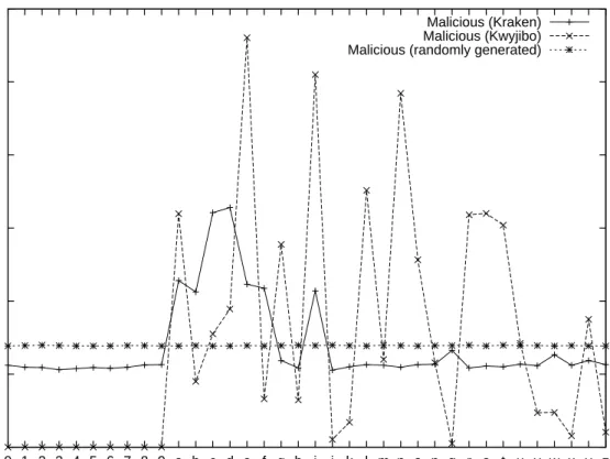
2. Even the most sophisticated algorithmic domain generator seen in the wild for Kraken botnet has a fairly uniform distribution, albeit with higher frequencies at the vowels: ‘a’, ‘e’ and ‘i’.
3. If botnets of future were to evolve and construct words that are pronounceable yet not in the dictionary, then they would not exhibit a uniform distribution as expected. For instance, Kwyjibo exhibits higher frequencies at alphabets, ‘e’, ‘g’, ‘i’, ‘l’, ‘n’, etc. In this regards, techniques that are based on only the distribution of unigrams (single alphanumeric characters) may not be sufficient, as we will show through the rest of this section.
0 0.02 0.04 0.06 0.08 0.1 0.12 0.14 0 5 10 15 20 25 30 35 Probability of occurrence
Alphanumeric character index (0-9, a-z)
Non-malicious (ISP dataset) Non-malicious (DNS dataset) Malicious (randomly generated) Malicious (Kraken) Malicious (Kwyjibo)
Fig. 1. Probability distribution of alphanumeric characters for mali-cious/non-malicious datasets.
0 0.02 0.04 0.06 0.08 0.1 0.12 0 1 2 3 4 5 6 7 8 9 a b c d e f g h i j k l m n o p q r s t u v w x y z Probability of occurrence Alphanumeric characters Malicious (Kraken) Malicious (Kwyjibo) Malicious (randomly generated)
Fig. 2. Probability distribution of alphanumeric characters for malicious datasets.
The terminology used in this and the following Chapters is as follows. For a hostname such asphysics.university.edu, we refer touniversity as the first-level sub-domain, edu as the top-level domain, and university.edu as the first-level domain. Similarly,physics.university.edu is referred to as the second-level domain andphysics
is the second-level sub-domain.
3.2 Metrics for anomaly detection
The K-L(Kullback-Leibler) divergence metric is a non-symmetric measure of ”dis-tance“ between two probability distributions. The divergence (or distance) between two discretized distributions P and Q is given by:
DKL(P||Q) =
Pn
i=1P(i)log P(i) Q(i).
where n is the number of possible values for a discrete random variable. The probability distribution P represents the test distribution and the distribution Q
represents the base distribution from which the metric is computed.
Since the K-L measure is asymmetric, we use a symmetric form of the metric, which helps us deal with the possibility of singular probabilities in either distribution. The modified K-L metric is computed using the formula:
Dsym(P Q) = 12(DKL(P||Q) +DKL(Q||P)).
Given a test distribution q computed for the domain to be tested, and non-malicious and non-malicious probability distribution over the alphanumerics as g and b respectively, we characterize the distribution as malicious or not via the following optimal classifier. For the test distribution q to be classified as non-malicious, we expect Dsym(qg) to be less than Dsym(qb). However, if Dsym(qg) is greater than
Dsym(qb), the distribution is classified as malicious.
3.2.1 Measuring K-L divergence with unigrams
The first metric we design measures the KL-divergence of unigrams by considering all domain names that belong to the same group, e.g. all domains that map to the same IP-address or those that belong to the same top-level domain. We postpone discussion of groups to Section IV. Given a group of domains for which we want to establish whether they were generated algorithmically or not, we first compute the distribution of alphanumeric characters to obtain the test distribution. Next, we compute the KL-divergence with a good distribution obtained from the non-malicious data sets (ISP or DNS crawl) and a malicious distribution obtained by modeling a botnet that generates alphanumerics uniformly. As expected, a simple unigram based
technique may not suffice, especially to detect Kraken or Kwyjibo generated domains. Hence, we consider bigrams in our next metric.
3.2.2 Measuring K-L divergence with bigrams
A simple obfuscation technique that can be employed by algorithmically generated malicious domain names could be to generate domain names by using the same dis-tribution of alphanumerics as commonly seen for legitimate domains.
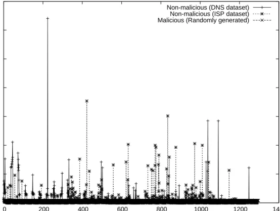
0 0.01 0.02 0.03 0.04 0.05 0.06 0.07 0 200 400 600 800 1000 1200 1400 Probability of occurrance Bigram index Non-malicious (DNS dataset) Non-malicious (ISP dataset) Malicious (Randomly generated)
Fig. 3. Probability distribution of bigram indices for legitimate and malicious datasets.
Hence, in our next metric, we consider distribution of bigrams,i.e., two consecu-tive characters. We argue that it would be harder for an algorithm to generate domain names that exactly preserve a bigram distribution similar to legitimate domains since
the algorithm would need to consider the previous character already generated while generating the current character. The choices for the current character will be hence more restrictive than when choosing characters based on unigram distributions.
Analogous to the case above, given a group of domains, we extract the set of bigrams present in it to form a bigram distribution. Note that for the set of alphanu-meric characters that we consider [a-z,0-9], the total number of bigrams possible are 36x36, i.e., 1,296. The probability distribution of bigrams for both the legitimate and malicious domains are shown in Figure 3. Our improved hypothesis now involves validating a given test bigram distribution against the bigram distribution of non-malicious and non-malicious sub-domains. We use the database of non-non-malicious words to determine a non-malicious probability distribution. For a sample malicious distri-bution, we generate bigrams randomly. Here as well, we use KL-divergence over the bigram distribution to determine if a test distribution is malicious or legitimate.
3.2.3 Edit distance
Note that the two metrics described earlier, rely on definition of a “good” distribution (KL-divergence). Hence, we define a third metric, Edit distance, which classifies a group of domains as malicious or legitimate by only looking at the domains within the group, and is hence not reliant on definition of a good database or distribution. The Edit distance between two strings represents an integral value identifying the number of transformations required to transform one string to another. It is a sym-metric measure and provides a measure of intra-domain entropy. The type of eligible transformations are addition, deletion, and modification. For instance, to convert the wordcat todog, the edit distance is 3 as it requires all three characters to be replaced. With reference to determining anomalous domains, we expect that all sub-domains (or hostnames) which are randomized, will, on an average, have higher edit distance
value. We use the Levenshtein edit distance dynamic algorithm for determining the edit distance , as shown in algorithm in 1 [28].
Algorithm 1Dynamic programming algorithm for finding the edit distance
EditDist(s1,s2) 1. int m[i,j] = 0 2. fori ←1to|s1| 3. dom[i,0] =i 4. forj ←1to|s2| 5. dom[0,j] =j 6. fori ←1to|s1| 7. do forj ←1to|s2|
8. dom[i,j] = min{m[[i-1,j-1] + if(s1[i] =s2[j]) then 0 else 1 fi,
9. m[i-1,j] + 1
10. m[i,j-1] + 1}
CHAPTER IV
GROUPING DOMAIN NAMES
In this Chapter, we present ways by which we group together domain names in order to compute metrics that were defined in Chapter III earlier.
4.1 Per-domain analysis
Note that botnets such as Conficker used several first-level domain names to generate algorithmic domain names, e.g., .ws, .info, .org. Hence, one way by which we group together domain names is via the first-level domain name. The intention is that if we begin seeing several algorithmically generated domain names being queried such that all of them correspond to the same first-level domain, then this may be reflective of a few favorite domains being exploited. Hence for all domains,e.g.,abc.examplesite.org, def.examplesite.org,etc., that have the same first-level domain nameexamplesite.org, we compute all the metrics over the alphanumeric characters and bigrams. Since domain fluxing involves a botnet generating a large number of domain names, we consider only domains which contain a sufficient number of second-level sub-domains,
e.g., 50, 100, 200 and 500 sub-domains.
4.2 Per-IP analysis
As a second method of grouping, we consider all domains that are mapped to the same IP-address. This would be reflective of a scenario where a botnet has registered several of the algorithmic domain names to the same IP-address of a command-and-control server. Determining if an IP address is mapped to several such malicious
domains is useful as such an IP-address or its corresponding prefix can be quickly blacklisted in order to sever the traffic between a command-and-control server and its bots. We use the dataset from a Tier-1 ISP to determine all IP-addresses which have multiple hostnames mapped to it. For a large number of hostnames representing one IP address, we explore the above described metrics, and thus identify whether the IP address is malicious or not.
4.3 Component analysis
A few botnets have taken the idea of domain fluxing further and generate names that span multiple TLDs, e.g., Conficker-C generates domain names in 110 TLDs. At the same time domain fluxing can be combined with another technique, namely “IP fluxing” [1] where each domain name is mapped to an ever changing set of IP-addresses in an attempt to evade IP blacklists. Indeed, a combination of the two is even harder to detect. Hence, we propose the third method for grouping domain names in to connected components.
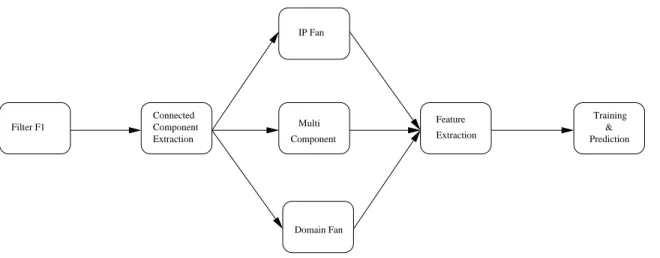
Connected Component Extraction Extraction Training Prediction & Feature Filter F1 IP Fan Domain Fan Multi Component
The analysis of components is done over five stages as shown in Figure 4. Each of the five stages are explained in detail below:
4.3.1 Filter F1
We use this filter to reduce the traffic into the stage 2 onwards in Figure 4 without losing much information. Most of the botnet groups and other groups involved in malicious activity would either return multiple hosting servers as a reply for a domain name or multiple domains are hosted on a single server. After experimentation we use a threshold of 5 since we do not lose much useful information and at the same time we also get a considerable reduction in the trace size. The input to this trace is the complete set of (IP address, domain name) tuples from all the DNS replies for ”Name Service” present in the trace. The following cases are the two cases of interest to us:
1. A given domain name returning more than 5 IP addresses. This will result in two component classes namely Multi component and Domain Fans which are explained in detail below.
2. A given IP address is mapped to more than 5 domain names. This constraint is mainly used for the IP fan component class which is explained in detail below.
4.3.2 Connected component extraction
The second stage splits the traffic into three different categories each of which analyzed separately. We use a connected component extraction of the bi-partite graph of IP-addresses and domain names. By definition a connected component is isolated and will not have a connecting edge to any other component. The extraction of connected components is explained in detail below: We construct a bipartite graph G with
IP-addresses on one side and domain names on the other. An edge is constructed between a domain name and an IP-address if that IP-address was ever returned as one of the responses in a DNS query. When multiple IP addresses are returned, we draw edges between all the returned IP addresses and the queried host name.
First, we determine the connected components of the bipartite graphG, where a connected component is defined as one which does not have any edges with any other components. Next, we compute the various metrics (KL-divergence for unigrams and bigrams, Edit distance) for each component by considering all the domain names within a component.
The number of connected components in the graph Gis given by the number of trivial eigen vectors of the graph Laplacian L(G) = D−W where the matrices D and W are as defined below.
The component analysis analyzes the connected components of this graph. Each connected component of this graph reveals the interconnected nature of the IP ad-dresses and the domain names these adad-dresses support. By definition, a connected component is not connected to another connected component and hence has no com-mon IP address or a comcom-mon domain name. Let ip = I be the total number of IP-addresses that are present after the F1 stage. and let d = D be total number of domain names that are present after the F1 stage. The vertices of graph Gcomprise of all IP-addresses and domains, for a total of (I +D) vertices. First, define the weighted adjacency matrix of the graph G as the matrix W = (wij) where i and j
are indices to the set of IP-addresses and domain names respectively. The degree of a vertex vi is defined as di =
Pn
j=1wij. Note that, in fact, this sum only runs
over all vertices adjacent to vi, as for all other vertices vj the weight wij is 0. The
degree matrix Dis defined as the diagonal matrix with the degrees d1,· · · , dn on the
with values A(i, j) = 1 or = 0 if the IP-address was mapped to that domain name. Eigen value decomposition of the Graph Laplacian allows us to compute the number of connected components quite easily as the number of trivial eigen vectors (eigen value = 0). While the corresponding vectorsU and V provide the IP-addresses and domain names that are part of the corresponding connected component. The algo-rithm for the connected component extraction is as shown in Algoalgo-rithm 4.3.2. We perform a DFS on each node to search for an existing link to another vertex and recurse through all the nodes to separate the connected components. At the end of this algorithm we would get a matrix comprising sub-matrices of all the connected components present in the input set of vertices.
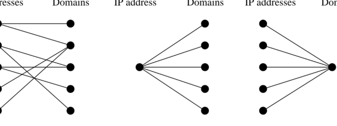
IP addresses Domains IP addresses
Multi Component
IP Fan
Domain Fan
Domains
IP address Domain
Fig. 5. Different component classes.
4.3.3 Component separation
Component extraction separates the IP-domain graph into components which can be classified in to different classes as shown in Figure 5. Each of the classes are explained in detail below:
Algorithm 2Algorithm to extract the connected components procedureConnectedCompExtraction(A, i, j)
1: index = 0 {// DFS node number counter} 2: S = empty {// An empty stack of nodes} 3: for all v in V do
4: if v.index is undefined then 5: { // Start a DFS at each node} 6: tarjan(v) {// we haven’t visited yet} 7: end if
8: end for
9: procedure tarjan(v)
10: v.index = index {// Set the depth index for v} 11: v.lowlink = index
12: index = index + 1
13: S.push(v) {// Push v on the stack} 14: for all (v, v’) in E do
15: {// Consider successors of v} 16: if v’ index is undefined then 17: { // Was successor v’ visited?} 18: tarjan(v’) {// Recurse}
19: v.lowlink = min(v.lowlink, v’.lowlink) 20: else if v’ is in S then
21: { // Was successor v’ in stack S?} 22: v.lowlink = min(v.lowlink, v’.index ) 23: end if
1. IP fan: these have one IP-address which is mapped to several domain names. Besides the case where one IP-address is mapped to several algorithmic domains, there are several legitimate scenarios possible. First, this class could include domain hosting services where one IP-address is used to provide hosting to several domains, e.g. Google Sites, etc. Other examples could be mail relay service where one mail server is used to provide mail relay for several MX domains. Another example could be when domain registrars provide domain parking services, i.e., someone can purchase a domain name while asking the registrar to host it temporarily.
2. Domain fan: these consist of one domain name connected to multiple IPs. This class will contain components belonging to the legitimate content providers such as Google, Yahoo!, etc. Since we do not have multiple domain names belonging to a given class, we would build a component based on the second level domain names. If we wait long enough then the legitimate components in this class may find an edge to their corresponding legitimate components in the multi-component class. All the domain names and IP addresses belonging to a particular legitimate component will likely converge into one big component in the multi-component class. To analyze the components in this class, we collapse all the domain names based on the second level domain name and the Top Level Domain(TLD). We collect the features for each such second level domain name and TLD, i.e. we would compute the average of the features for all the domain names belonging to such a second level domain name and TLD. For example aaa.xyz.com, bbb.xyz.com, ccc.xyz.com would be the domain names for the second level domain name of xyz.com. At times a few of the IP addresses would end up in this component class because of a shortage in the
analysis period, given enough time ideally all the IP addresses (hosting server) of a single business unit would end up in a single component. Due to shortage in analysis period, a few of such split up components would be present in this component class.
3. Multi component: these are components that have multiple IP addresses and multiple domain names, e.g., Content Distribution Networks (CDNs) such as Akamai. This is the class which contains most part of information in the trace. Various parameters not directly related only to the domain names can be com-puted only in this component class. A few such examples are IP growth ratio, IP degree (average number of IPs hosting a given domain name), domain de-gree (average number of domain names hosted in an IP address) etc. A lot of legitimate service providers like Google, Yahoo etc. would also be present in this component class. A few domain names of these legitimate service providers would be hosted on multiple servers around the world. This distribution of contenet over multiple servers is mainly done for load balancing and also for content distribution.
Most of the botnets involve in both “IP fluxing” and “Domain fluxing”. These botnet groups would register a new IP address every few days, this would result in “IP fluxing” and since these botnet groups are also known to register new domain names every few hours this would register in “Domain fluxing”. We would need to detect such components which involve in both “IP fluxing” and “Domain fluxing”.
4.3.4 Feature extraction
All the features/metrics explained in Section III are computed for all the components extracted in Stage 2 as shown in Figure 4. To compute the feature value for each of the components extracted, we would compute the metrics individually for each of the domain names belonging to the component. Then we would take the average of all the domain names in the component to compute the feature value of the component.
4.3.5 Training and prediction
Note that the problem of classifying a component as malicious (algorithmically gen-erated) or legitimate can be formulated in a supervised learning setting as a linear regression or classification problem. In particular, we label the components and train a L1-regularized Linear Regression over 10 hours out of the one day of the ISP trace we have access to. We first label all domains within the components found in the training data set by querying against domain reputation sites such as McAfee Site Advisor [29] and Web of Trust [30] as well as by searching for the URLs on search-engines [31]. Next, we label a component as good or bad depending on a simple majority count, i.e., if more than 50% of domains in a component are classified as malicious (adware, malware, spyware, etc.) by any of the reputation engines, then we label that component as malicious.
Define the set of features as F which includes the following metrics computed for each component: KL-distance on unigrams, KL-distance on bigrams and Edit distance. Also define the set of Training examples as T and its size in terms of number of components as |T|. Further, define the output value for each component yi = 1 if it was labeled malicious or = 0 if legitimate. We model the output value
feature where the weights are given byβj for each featurej ∈F: yi =
P
j∈F βjxj+β0
In particular, we use the LASSO, also known as L1-regularized Linear Regression [32], where an additional constraint on each feature allows us to obtain a model with lower test prediction errors than the non-regularized linear regression since some vari-ables can be adaptively shrunk towards lower values. The value of the regularization parameter λ∈ [0-1] that provides the minimum training error (equation below) and then use thatλ value in our tests:
argmin β |T| X i=1 (yi−β0− X j∈F βjxj)2+λ X j∈F |βj|. (4.1)
This value of regularization parameterλis used during the prediction stage. The feature values of the all the componenents to be predicted is given as the input value to the linear regression model. If the output valueyi of this regression model for the
test component is greater than the threshold value chosen, then this component is marked as suspicious.
The metrics that we use for prediction namely K-L distance of unigrams and bigrams and Edit Distance would require a minimum of a few domain names to predict with a higher accuracy as described in the Chapter III. During prediction, we would consider only components which have more number of domain names than the threshold we find experimentally. To verify the exact nature of the component we check the various domain names in the component against existing blacklisting services and we also manually check for each of the domain names in the internet.
CHAPTER V
RESULTS
In this Chapter, we present results of employing various metrics across different groups, as described in Chapter III. We briefly describe the data set used for each experiment.
5.1 Per-domain analysis 5.1.1 Data set
The analysis in this sub-section [33] is based only on the sub-domains belonging to a domain. The non-malicious distribution g may be obtained from various sources. For our analysis, we use a database of DNS PTR records corresponding to all IPv4 addresses. The database contains 659 first-level domains with at least 50 second-level domains, while there are 103 first-level domains with at least 500 second-level sub-domains. From the database, we extract all first-level domains which have at least 50 second-level sub-domains. All second-level sub-domains corresponding to such domains are used to generate the distribution g. For instance, a first-level domain such asuniversity.edu may have manysecond-level sub-domains such as physics,cse,
humanities etc. We use all such sub-domains that belong to trusted domains, for determiningg.
To generate a malicious base distributionb, we randomly generate as many char-acters as present in the non-malicious distribution. We use sub-domains belonging to well-known malware based domains identified by Botlab, and also a publicly available webspam database as malicious domains [34] for verification using our metrics.
Bot-lab provides us with various domains used by Kraken, Pushdo, Storm, MegaD, and Srizbi. Forper-domain analysis, the test words used are the second-level sub-domains. Figure 1 shows how malicious/non-malicious distributions appear for the DNS PTR dataset as well as the ISP dataset described in the following sections.
5.1.2 K-L divergence with unigram distribution
We measure the symmetrized K-L distance metric from the test domain to the malicious/non-malicious alphabet distributions.
It is observed that with lower number of samples, the number of sub-domains required for accurate detection corresponds to the latency of accurately classifying a previously unseen domain. The results [10] seem to point out that a domain-fluxing domain can be accurately characterized by the time it generates 500 names or less.
5.1.3 K-L divergence with bigram distribution
It is observed that a minimum of 200 to 500 sub-domains are required to yield good results with minimal false positives. We note that the performance with unigram distributions [10] is slightly better than using bigram distributions. This phenomena is particularly evident for experiments using 50/100 sub-domains. The false positive rates are seen to be slightly higher for bigram distributions compared to the unigram distributions.
However, when botnets employ counter measures to our techniques, the bigram distributions may provide better defense compared to unigram distributions as they require more effort to match the good distribution (g).
5.1.4 Edit distance of sub-domains
Figure 6 shows the performance using edit distance as the evaluation metric. The area under the ROC is a measure of the goodness of the metric. We observe that with 200 or 500 sub-domains, we cover a relatively greater area, implying that using many sub-domains helps obtain accurate results. The detection rate for 50/100 test words reaches 1 only for high false positive rates, indicating that a larger test word set should be used. For 200/500 sub-domains, 100% detection rate is achieved at false positive rates of less than 0.1%. It is observed with all the measures that we can settle for a relatively low false positive rate with a good detection rate when we have relatively high sub-domains like 200 to 500.
0.1 1
0.01 0.1 1
True positive rate (TPR)
False positive rate (FPR)
Using 50 test words Using 100 test words Using 200 test words Using 500 test words
0.1 1
0.001 0.01 0.1 1
True positive rate (TPR)
False positive rate (FPR)
Using 50 sub-domains Using 100 sub-domains Using 200 sub-domains Using 500 sub-domains
Fig. 7. ROC curve : K-L metric with bigram distribution (Per-IP).
5.2 Per-IP analysis 5.2.1 Data set
Here, we present the evaluation [33] of domain names that map to an IP address. For analyzing the per-IP group, for all hostnames mapping to an IP-address, we use the sub-domains except the top-level domain TLD as the test word. For instance, for hostnames physics.university.edu and cse.university.edu mapping to an IP address, say 6.6.6.6, we use physicsuniversity and cseuniversity as test words. However, we only consider IP addresses with at least 50 hostnames mapping to it. We found 341 such IP addresses, of which 53 were found to be malicious, and 288 were considered non-malicious. The data is obtained from DNS traces of a Tier-1 ISP in Asia.
Many hostnames may map to the same IP address. Such a mapping holds for botnets or other malicious entities utilizing a large set of hostnames mapping to fewer C&C(Command and Control) servers. It may also be valid for legitimate internet service such as for Content Delivery Networks (CDNs). We first classify the IPs obtained into two classes of malicious and non-malicious IPs. The classification is done based on manual checking, using blacklists, or publicly available Web of Trust information [30]. We manually confirm the presence ofConficker based IP addresses and domain names [3]. The ground truth thus obtained may be used to verify the accuracy of classification. Figure 1 shows the distribution of non-malicious test words and the randomized distribution is generated as described previously.
5.2.2 Results
We discuss the results of per-IP analysis below. For the sake of brevity, we present results based on K-L distances of bigram distributions as shown in Figure 7. Summary of results from other metrics is provided.
The ROC curve for K-L metric shows that bigram distribution as shown in Figure 7 can be effective in accurately characterizing the domain names belonging to different IP addresses. We observe a very clear separation between malicious and non-malicious IPs with 500, and even with 200 test words. With a low false positive rate of 1%, high detection rates of 90% or more obtained with 100 or more test words. The bigram analysis was found to perform better than unigram distributions. The per-IP bigram analysis performed better than per-domain bigram analysis. We believe that the bigrams obtained from the ISP dataset from Asia provide a compre-hensive non-malicious distribution. The first-level sub-domains also assist in discard-ing false anomalies, and therefore providdiscard-ing better performance.
in general. The experiments with 100 test words results in a low false positive rate of about 10% for a 100% detection rate. However for using only 50 test words, the detection rate reaches about 80% for a high false positive rate of 20%. Thus, we conclude that for per-IP based analysis, the JI measure performs relatively better than previous measures applied to this group. However, as highlighted in section VI, the time taken to compute edit distance is large.
5.3 Component analysis results 5.3.1 Methodology
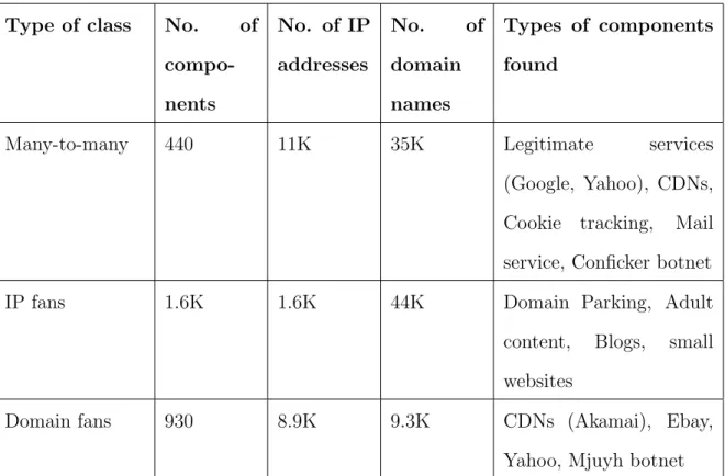
We discuss the results from applying connected component analysis to the ISP trace. We classify the connected components in to three classes: IP fans, Domain fans and Many-to-many components, details of which are provided in Table I.
Next, we use a supervised learning framework where we train a L1-regularized linear regression model (see Equation 4.1) on components labeled in a 10-hour trace interval. For labeling the components during training, we used the information from URL reputation services such as Web of Trust, McAfee Site Advisor and mark 128 components as good (these contain CDNs, mail service providers, large networks such as Google) and we mark 1 component belonging to the Conficker botnet as malicious. For each component we compute the features of KL-divergence, Jaccard Index measure and Edit distance. We train the regression model using glmnet tool [32] in statistical package R, and obtain the value for the regularization parameterλ as 1e−4, that minimizes training error during the training phase. We then test the model on the remaining portion of the one day long trace. In this regards, our goal is to check if our regression model can not only detect Conficker botnet but whether it can also detect other malicious domain groups during the testing phase over the trace.
Table I. Different types of classes
Type of class No. of compo-nents No. of IP addresses No. of domain names Types of components found
Many-to-many 440 11K 35K Legitimate services
(Google, Yahoo), CDNs, Cookie tracking, Mail service, Conficker botnet
IP fans 1.6K 1.6K 44K Domain Parking, Adult
content, Blogs, small websites
Domain fans 930 8.9K 9.3K CDNs (Akamai), Ebay,
Yahoo, Mjuyh botnet
We apply a constraint, requiring a minimum of 20 domain names per component to predict with more confidence. During the testing stage, if a particular component is flagged as suspicious then we check against Web of Trust [30], McAfee Site Advisor [29] as well as via Whois queries, search engines, to ascertain the exact behavior of the component.
5.3.2 Results
Detailed results for each of the component class are as shown in Table I and II. The details of each of the groups of components extracted is given below later we explain
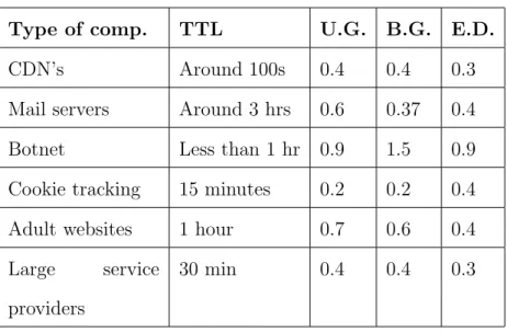
Table II. Behavior of the type of component
Notation
TTL Time To Live
U.G. K.L. Divergence of Unigrams
B.G. K.L. Divergence of Bigrams
E.D. Edit Distance
Type of comp. TTL U.G. B.G. E.D.
CDN’s Around 100s 0.4 0.4 0.3
Mail servers Around 3 hrs 0.6 0.37 0.4
Botnet Less than 1 hr 0.9 1.5 0.9
Cookie tracking 15 minutes 0.2 0.2 0.4
Adult websites 1 hour 0.7 0.6 0.4
Large service providers
30 min 0.4 0.4 0.3
the results from each of the component classes.
The characteristics of each such groups are as shown in Table II. The behavior of each of these classes are explained below:
1. It can be observed that the CDN’s and large service providers like Google have a very low value of TTL, this is done for load balancing. With a low value of TTL, the DNS servers can return an updated set of hosting servers with time. For example say the CDN’s provide service for both a news website like CNN and a sports channel like Fox Sports on the same set of servers. During normal
Table III. Detailed results for each class
Notation
U.G. K.L. Divergence of Unigrams
B.G. K.L. Divergence of Bigrams
E.D. Edit Distance
Type Multi component IP fans Domain fans
Feature U.G. B.G. E.D U.G. B.G. E.D U.G. B.G. E.D
Training Conficker component -
-Detected com-ponents 10 1 3 - - 14 - - 1 Detected no. of domain names 2229 1908 2082 - - 510 - - 121 False Positive components 2 3 - - - 1 - - -False Positive no. of domain names 99 12920 - - - 56 - -
-traffic say both these services are hosted on the same set of servers. When the traffic is high from one of the clients say during a football match when the traffic is very high from the sports channel. To provide fair service to other clients like say the news websites initially hosted with the sports websites, the fair server allocator would allocate new servers to such low traffic clients. This way all the clients subscribing to these CDNs would be given a fair service.
2. The mail servers would generally have a high TTL value since they would gener-ally have a single server providing service to multiple clients. Their edit distance value would be on the higher side since they provide service to a variety of end user kind of clients who would not have any common part in the domain name.
3. It can be observed that the groups which use algorithmically generate domain names has a very high value of KL-Divergence of unigrams and bigrams and Edit Distance.
4. Cookie tracking websites would track the cookies and predict the advertisements for a given user based on his browsing. Private websites would use the service of these websites to suggest advertisements/products to such users.
5. Adult websites use a slightly longer TTL since they would not change their servers frequently. Also their edit distance would be high since they would host the same content under different domain names on the same server. This is mainly done to attract more users.
The results from each of these component classes are described below:
1. Multi component: This is the biggest class which has most of the information in the trace. There are a total of 442 components components in this component class having a total of 11.1K IP addresses and 34.9K domain names as shown
in Table I. The number of domain names in a component vary from 12.8K (psmtp mail relays) to 2 (small networks). A few of the components present in this component class are the CDN, large service providers like google, mail providers, cookie tracking, botnet groups etc.
If we use Edit distance as the feature we correctly predict 3 components (Con-ficker, 1 component with tricked names, 1 component hosting adult content). There are no false positives with this feature. If we use KL-divergence with bigrams as the feature for prediction only Conficker component is correctly predicted along with 3 other false positives (Cloudfront, mail relay services). These false positives can be eliminated using other features (such as TTL). KL-Divergence with unigrams as a feature correctly predicts 10 components (1 Conficker, 1 malware/bot, 5 mis-spelt, 3 adult content). There are two false positives(1 google, 1 news blogs). Each of these type of detected components are explained in detail later in this section.
2. IP Fans: The number of domains in this class varies from 66 (domain parking) to 5 (small enterprises and adult websites). If we use edit distance as the feature 15 components (630 domain names) are correctly predicted for domain parking out of 1605 components with no false positives.
3. Domain Fans: In this class, we find 430 second level domains for which we employ all the features. The number of domain names corresponding to these second level domains varies from 121 (bot) to 1 (small networks). When we use edit distance as the feature, there is only 1 component with a second level domain which gets detected out of the present 430 second level domains. We do not detect anything using alphabet entropy and bigram frequency in this class.
Table IV. Summary of interesting networks discovered through component analysis
Component Type No. of Com-ponents No. of do-mains No. of IPs Conficker botnet 1 1.9K 19 Helldark botnet 1 28 5 Mjuyh botnet 1 121 1.2K Misspelt Domains 5 215 17 Domain Parking 15 630 15 Adult content 4 349 13
3K components) are classified as malicious, and we find 27 of them to be malicious after cross checking with external sources (Web of Trust, McAfee, etc.) while 2 components (99 domains) are false positives and comprise of Google and domains belonging to news blogs. Note that here we use a broad definition of malicious domains as those that could be used for any nefarious purposes on the web, i.e., we do not necessarily restrict the definition to only include botnet domain generation algorithm. Out of the 27 components that were classified as malicious, one of them corresponds to the Conficker botnet, which is as expected since our training incorporated features learnt from Conficker. We next provide details on the remaining 26 components that were determined as malicious (see Table IV). Next, we explain the results of each of the detected set of groups individually.
1. Mjuyh Botnet: The most interesting discovery from our component analysis is that of another Botnet, which we call Mjuyh, since they use the domain name
mjuyh.com (see Table V). The second level name is generated randomly and is 57 characters long. Each of the 121 domain names belonging to this bot network return 10 different IP addresses on a DNS query for a total of 1.2K IP-addresses. Also, in some replies, there are invalid IP addresses like 0.116.157.148. All the 10 IP addresses returned for a given domain name, belong to different network prefixes. Furthermore, there is no intersection in the network prefixes between the different domain names of the mjuyh bot. We strongly suspect that this is case of “domain fluxing” along with “IP fast fluxing” going on, where each bot generated a different randomized query which was resolved to a different set of IP-addresses.
2. Helldark Trojan: We discovered a component containing 5 different second level domains (a few sample domain names are as shown in Table V) The component comprises of 28 different domain names which were all found to be spreading multiple Trojans. One such Trojan spread by these domains is Win32/Hamweq.CW that spreads via removable drives, such as USB memory sticks. They also have an IRC-based backdoor, which may be used by a remote attacker to order the affected machine to participate in Distributed Denial of Service attacks, or to download and execute arbitrary files [35].
3. Mis-spelt component: There are about 5 components (comprising 220 domain names) which used tricked (mis-spelt or slightly different spelling) names of reputed domain names. For example, these components use domain names such as uahoo.co.uk to trick users trying to visit yahoo.co.uk (since the alphabet ‘u’ is next to the alphabet ‘y’, they expect users to enter this domain name by mistake). Dizneyland.com to trick users trying to visit Disneyland.com (which replaces the alphabet ‘s’ with alphabet ‘z’). We still consider these components
Table V. Domain names used by bots
Type of group Domain names
Conficker botnet vddxnvzqjks.ws gcvwknnxz.biz joftvvtvmx.org Mjuyh bot 935c4fe60462ea17126904272149--c258a35bfc3ed65528431555c03d.6.mjuyh.com c2d026e07295e8f3fefa771a049b804--45c353bdd55c3d1342b823350.6.mjuyh.com Helldark Trojan may.helldark.biz X0R.ircdevils.net www.BALDMANPOWER.ORG Domain Parking realdealreport.com ghostzilla.com abolishthesenate.org Legitimate Domains dkz2f4f37vdc9.hkg1.cloudfront.net ltvxid5qpnjfsxuwefrckbv0sb.Megavideo.com
as malicious since they comprise of domains that exhibit alphanumeric features different than normal.
4. Domain Parking: We found 15 components (630 domain names) that were being used for domain parking, i.e., a practice where users register for a domain name without actually using it, in which case the registrar’s IP-address is returned as the DNS response. In these 15 components, one belongs to GoDaddy (66 domain names), 13 of them belong to Sedo domain parking (510 domain names) and one component belongs to OpenDNS (57 domain names). Clearly these components represent something out of the normal as there are many domains with widely disparate algorithmic features clustered together on account of the same IP-address they are mapped to.
5. Adult Content: We find four components that comprise of 349 domains primar-ily used for hosting adult content sites. Clearly this matches the well known fact, that in the world of adult site hosting, the same set of IP-addresses are used to host a vast number of domains, each of which in turn may use very different words in an attempt to drive traffic.
In addition, for comparison purposes, we used the lexical features of the domain names such as the length of the domain names, number of dots and the length of the second level domain name (xyz.com, for example) for training on the same ISP trace instead of the KL-divergence and Edit distance measures used in our study. These lexical features were found to be useful in an earlier study in identifying malicious URLs [12]. The model trained on these lexical features correctly labeled four com-ponents as malicious (Conficker bot network, three adult content comcom-ponents and one component containing mis-spelt domain names) during the testing phase, but it also resulted in 30 components which were legitimate as being labeled incorrectly;
compare this against 27 components that were correctly classified as malicious and two that were false positives on using our alphanumeric features.
We also test our model on an ISP Tier 1 trace from Brazil. This trace is about 20 hours long and is collected on a smaller scale as compared to the ISP trace from Asia. This trace from Brazil was collected 15 days after the ISP trace from Asia was collected. We use the same training set for the prediction model as we had used for the ISP trace from Asia. In the prediction stage we successfully detect the Conficker component with no false positives. We are not able to detect other components because the length of the trace is smaller in size as compared to the other trace. The Conficker component has 185 domain names and 10 IP addresses. 9 out of the 10 IP addresses are common between this component and the Conficker component from the ISP trace from Asia. So we could definitely say that the servers do not change much with time. But out of the 185 domain names only 5 domains are common from this component and the component from the ISP trace from Asia. This clearly shows the domain fluxing in Conficker botnet.
CHAPTER VI
DISCUSSION
6.1 Usefulness of component analysis
Conficker botnet, present in our ISP trace, employs domain fluxing across TLDs, that became directly visible after IP-domain components were extracted and analyzed from the trace. The component analysis allowed the application of our detection methods across several different domains, which otherwise would have looked different from each other. In addition, component analysis allowed us to detect Conficker domains that would not have been detectable with our approach when applied to domain names alone since some of these domains contained fewer than 50 names needed for accurate analysis. Similarly, some of the IP addresses in the component hosted fewer than 50 names and would not have been detected with the IP address based analysis either. However, these domains will be included in the component analysis as long as the component has altogether more than 50 names.
LetDc be the number of hostnames andIcbe the number of IP addresses in the
component. If Dd, Id are the number of hostnames and corresponding IP addresses
detected through domain level analysis, we define domain level completeness ratios as Dd/Dc and Id/Ic. Similarly, we can define the completeness ratios for IP-based
analysis as Di/Dc and Ii/Ic, where Di and Ii correspond to the total number of
hostnames and IP addresses of the conficker botnet detected by the IP-based analysis. For the Conficker botnet, these completeness ratios for IP-based analysis were 73.68% for IP addresses and 98.56% for hostnames. This implies that we are able to detect an additional 26.32% of IP addresses and a relatively small fraction of 1.44%
70 75 80 85 90 95 100 Per-domain Per-IP Percentage identification Type of analysis IPs identified Domains identified