Received 11 May 2016|Accepted 16 Aug 2016|Published 3 Oct 2016
Unsupervised vector-based classification
of single-molecule charge transport data
Mario Lemmer
1, Michael S. Inkpen
1, Katja Kornysheva
2, Nicholas J. Long
1& Tim Albrecht
1The stochastic nature of single-molecule charge transport measurements requires collection of large data sets to capture the full complexity of a molecular system. Data analysis is then guided by certain expectations, for example, a plateau feature in the tunnelling current distance trace, and the molecular conductance extracted from suitable histogram analysis. However, differences in molecular conformation or electrode contact geometry, the number of molecules in the junction or dynamic effects may lead to very different molecular signatures. Since their manifestation is a priori unknown, an unsupervised classification algorithm, making no prior assumptions regarding the data is clearly desirable. Here we present such an approach based on multivariate pattern analysis and apply it to simulated and experimental single-molecule charge transport data. We demonstrate how different event shapes are clearly separated using this algorithm and how statistics about different event classes can be extracted, when conventional methods of analysis fail.
DOI: 10.1038/ncomms12922 OPEN
1Department of Chemistry, Imperial College London, Imperial College Road, London SW7 2AZ, UK.2Institute for Cognitive Neuroscience, University College London, Alexandra House, 17-19 Queen Square, London WC1N 3AR, UK. Correspondence and requests for materials should be addressed to T.A. (email: [email protected]).
T
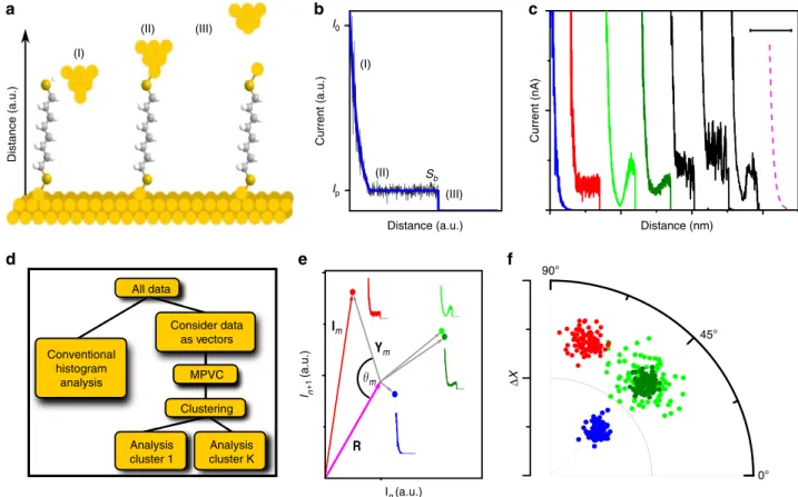
he first single molecular conductance measurements were performed in the 1990s. Since then, a variety of different methodologies to measure charge transport across single molecules have been established, including fixed, chip-based electrode nanogaps, mechanical break-junctions and scanning probe microscopy techniques like scanning tunnelling (STM) and conducting tip atomic force microscopies1–11.For example, in STM-based tunnelling current–distance (I(s)) spectroscopy, as illustrated in Fig. 1a (refs 4,12,13), an STM tip at a constant bias voltage Vbias is approached to the surface of a conductive substrate until a predefined set point tunnelling currentI0is reached. The substrate typically carries the adsorbed molecule of interest, which is capable of forming a stable molecular bridge between the two electrodes via suitable anchor groups. The tip is then pulled away, while the tunnelling current Iis recorded as a function of tip/substrate distances. For smalls,I is dominated by through-space tunnelling and decays exponentially with a characteristic decay constant b, Fig. 1b (region I)14. For larger s, charge transport through the bridge molecule is thought to dominate, implying that I remains approximately constant at the plateau current Ip, namely until the molecular bridge is fully extended (region II). Further increase
in s typically results in the rupture of the molecular bridge at some break-off distance sb and I drops to the corresponding through-space value (effectively zero or noise level in most cases, region III).Ipcan then be related to the molecular conductance, while sbis a measure for the maximum length of the molecular bridge15–17. After collecting a sufficiently large number of I(s) traces, histogram-based analysis is usually employed to extract the most probable values ofIpandsbfor a given molecular junction, that is from maxima in the histogram.
However, this approach is not without problem. First, as mentioned above, such an analysis relies on a particular signal shape (for example, a plateau feature) and hence an assumption about the expected outcome. If the signal shape is different or more complex, the meaning of a maximum in the corresponding histograms is less clear. Second, conventional histogram-based analysis has a strong focus on the most abundant class of signals (majority species) and sub-populations in the data may remain unnoticed.
To this end, it is now well-documented that even for seemingly simple molecular systems, such as Au/1,8-octanedithiol (ODT)/ Au (Fig. 1a), theI(s) data can contain a diversity of other shapes, such as slanted plateaus, non-linear and telegraphic noise a f e b Distance (a.u.) (I) (II) (III) Current (a.u.) Distance (a.u.) Ip I0 Sb (I) (II) (III) d I+1 n (a.u.) In (a.u.) m R Ym 0° 45° 90° Δ X Current (nA) Distance (nm) Im c All data Conventional histogram analysis Consider data as vectors Analysis cluster 1 MPVC Clustering Analysis cluster K
Figure 1 |I(s)spectroscopy and MPVC overview.(a) Schematic of theI(s)method with ODT in the junction, including three steps during junction formation and rupture. (b) SimulatedI(s)trace (blue) with added noise (black). Currents at (I) to (III) correspond to the three stages shown ina. (c) Blue, red, light green and dark green trace: SimulatedI(s)traces without plateau, with plateau and with non-linear plateau with high and low amplitude, respectively. Black traces: experimental traces for ODT. Dashed line (b¼1.0 Å1): simulated reference vectorR. Traces are offset for clarity. Scale bar, 1 nm. (d) Flow chart of the MPVC process, illustrating the philosophy behind MPVC. Conventional analysis is typically based on certaina prioriassumptions regarding the shape of theI(s) traces. This informs the methodology of the analysis, but can be misleading (see main text). MPVC:I(s) data are regarded as vectors. Vector properties are calculated and used as classifiers for a measure of similarity betweenI(s) traces; no prior assumptions are required. Similar traces are assigned to groups, based on suitable clustering algorithms. Physical interpretation of each group is the final step. (e) Vector representation of the four simulated traces shown inc, in two dimensions (using two data points from each trace) for illustration. In our data, eachI(s) trace hasN¼2,000 data points, resulting in the same number of dimensions in vector space. (Simplified) distance vectorYandyare shown for the plain plateau. The two green points represent two traces with similarDXandybut differenthr. (f) Representation in cylindrical coordinates (view alongzaxis), in principle involving allN dimensions in the data. Red, blue and green clusters illustrate different conductance clusters, separable byDXandy. The light and dark green data points feature similarDXandy, but differenthrvalues.
features, Fig. 1c (black traces)11,12,18–23. These may, for example, reflect the dynamics of the electrode surfaces, the molecular binding configuration, bond formation or rupture, molecular conformational changes, multiple (potentially transient) contact points between the electrodes and the molecule, and the presence of varying numbers of molecules in the junction11,12,24–31. Identifying and analysing these features of the I(s)trace is thus essential for a more complete fundamental understanding of the processes on the nanoscale.
Hence, there is a need to develop statistical tools for the analysis of single-molecule charge transport data that (i) do not make anya prioriassumptions with regards to the signal shape and assess similarity within a given data set and (ii) allow for ideally unsupervised analysis and classification of large data sets, in order to capture the statistical complexity of the molecular system, including event classes that occur with low probability.
Here we present such a methodology, based on a new multi-parameter vector-based classification process (MPVC). We demonstrate its capabilities for a diverse set of simulated, but realisticI(s) data, as well as actual experimental results for two molecular systems, namely ODT and OPE (a,o-dithiol termi-nated oligo phenylene(ethynylene)). Importantly, we show how MPVC is capable of identifying and extracting sub-populations in the data, where conventional methods of analysis fail.
Results
Vector-based data analysis. Vector-based classification methods are powerful tools for categorizing the data and have found widespread application in such fields as genetics, robotics and neuroscience32,33. Generally, they operate by regarding a data set, for example, an I(s)curve with N current values in the present case, as anN-dimensional vectorXn(n¼1...N); a total number of Mobservations thus results in a data matrixXn,m(m¼1...M) or, in shortXm(droppingnfor convenience). The Euclidean distance |DX| between the two vector points may then be used as a measure for similarity between different data sets m and m0, equation (1): DXm;m0 ¼jXm0Xmj ¼ 1 Kp ffiffiffiffiN ffiffiffiffiffiffiffiffiffiffiffiffiffiffiffiffiffiffiffiffiffiffiffiffiffiffiffiffiffiffiffiffiffiffiffiffi X n xn;m0xn;m 2 r ð1Þ whereKis an optional normalization constant (if required, so that 0rDXr1). IfXmandXm0are identical, thenDXm,m0is zero;
if they are very different, DXm,m0 is large. After calculating all
combinations of distances between theMdata sets, a distance or probability criterion may then be used to classify the data. The computational effort scales with (M1)M, according to the variation formula, and can be very significant for some of our larger data sets (for example, involving 70,000 traces, see below). In the case of I(s) data, however, we found the mutual distance criterion to be insufficient in many cases. A different, somewhat expanded methodology was required, which as we show below, significantly improved the classification performance.
In a first step, we defined an arbitrary,N-component reference vectorR, which generally depends on the data to be analysed. It could be determined self-consistently, based on some optimiza-tion parameter (for example, to maximize the variance of the existing data around R). We chose a vector with noise-free, exponentially decaying current–distance values, which is similar to the experimental data without molecular binding events (I0¼20 nA; decay coefficient b¼1 Å1), Fig. 1c (dashed, magenta line).
We then calculate three vector properties in relation to the data sets Xm and R, namely, the length of the difference
vectorDX¼|Ym|¼|XmR|; the angleymbetweenYmand R, equation (2),
cosðymÞ ¼ RYm R j j jYmj
ð2Þ and the reduced Hamming distance hr between vectors Yr,m¼Ym/abs(Ym) andR/abs(R). The Hamming distance is the minimum relative number of component exchanges that render two vectors identical34. That is, if two vectors are identical, then the Hamming distance is 0 (no change required); if all components differ, then the Hamming distance is 1 (every component in one vector needs to be changed). Note that abs(Ym) and abs(R) are vectors containing the absolute component values ofYmandR, that is, they are not the length of the vectorsYmand R, respectively. The component values ofYr,mandR/abs(R) are thus either 1, 0 or 1.
In relation to theI(s) data, these three parametersDXm,ymand hr,mmay be illustrated in the following way:DXmis a measure for the total variation of a given I(s) trace relative to the reference trace R, as described above. No distinction is made between positive and negative deviations fromRand thus two differently shapedI(s) traces could feature the sameDXmvalue. For example, current values in a given trace 1 may be slightly higher than R over all s, while values in a second trace 2 may be significantly higher thanRfor lowsand then much lower thanRat larges. However, the dot product betweenRandYhelps to differentiate these two cases, since positive and negative vector components cancel out. Thus, RY1aRY2, resulting in different angles
y1 and y2 between Y1 and Y2, and R in vector space (the denominator in equation (2) serves to normalize with regards to the vector lengths). Finally,hrhelps to quantify, how large a fraction of the I(s) values in a given trace lies above or belowR. For example, a thirdI(s) trace may oscillate aroundRin a way that DX2¼DX3 and y2¼y3, but with more data points aboveR than trace 2 (for exampleYr,3 has more ‘1’s thanYr,2). Thus,hr,2ahr,3and the two curves can be differentiated.
It should be stressed that the above choice of parameters, while sensible, is neither complete nor exhaustive. Other statistical properties of the I(s) traces, such as the centre-of-mass of the curve, could be used to in addition or instead of one of the three parameter defined above. Generally, if the number of classifiers is too small, the classification will lack specificity and a cluster in the multi-parameter representation will contain many different types
ofI(s) traces. On the other hand, a too large number of classifiers
may result in a large dispersion in the multi-parameter representation, rendering the identification of clusters more difficult. We found that the combination of DXm, ym and hr,m struck a good balance in this regard.
An important feature of the above MPVC algorithm, compared with conventional methods of analysis, is that it does not make
any a priori assumptions with regards to the signal shape, for
example, whether a plateau feature is present or not. Rather, it looks for similarities between the measured data sets, relative toR and based on the classifiers used. A large number of similar traces will thus produce regions of high point density in the (DX,y,hr) representation, which can then be clustered and processed for further analysis.
Notably, MPVC does not provide the physical interpretation. It is partly for this reason that we chose both complex simulated data and well-characterized experimental system, where the interpretation is (largely) known, as a benchmark for MPVC here. The former allows for detailed characterization of the classifica-tion results (misclassificaclassifica-tion, especially where there are multiple groups), while the latter facilitates the physical interpretation of the clusters.
Finally, we note that by using a common reference vector we avoid having to compute the pairwise distance matrix for allI(s) traces to determine similarity between traces. This effectively reduces the dimensionality of the data and is a significant advantage for large data sets (as for the ODT data with 70,000 traces, see below).
In the three-dimensional (DX,ym,hr,m) representation, a range of different clustering algorithms can be applied to group the data, including k-means and k-medoids clustering, distribution-or density-based algdistribution-orithms35, Gaussian mixture models or neural networks36,37. A flow chart of the MPVC is provided in Fig. 1d. In the present work, we first use a distribution-based approach to illustrate the contribution of each parameter, and then employ three-dimensional Gustafson–Kessel fuzzy clustering in the second part of the paper38.
Since both modulus DX and angle y emerge from the classification process, we found representation in polar (or rather cylindrical) coordinates most convenient, Fig. 1f. The resulting event clusters can possess different and characteristic shapes, depending on the underlying nature of the variation in the data (say, a normally distributed plateau height or telegraphic noise features during bridge formation) and the reference vector. This in turn affects the way the individual clusters are identified and bound. For example, in cases where the cluster shape is symmetric, a Gaussian fit of the DX, y or hr histograms is usually most straightforward and event clusters may be defined based on a probability criterion (for example, within±2s(95%) of the distribution mean). When the clusters are highly stretched or even semi-circular, which we found to be the case for the simulated data with normally distributed sb, density-based clustering methods may be preferable35.
To enhance the separation between event clusters, in particular at low (S/N) ratio, it can sometimes be advantageous to exclude segments of the I(s) curve and define a region-of-interest (RoI), for example, where through-space tunnelling is dominant (at smalls) or where the current is unlikely to contain well-defined, molecule-related information (s44molecular length). This also
reduces the computational cost, as we show below for a data set containing 70,000I(s) traces.
Results
Simulated data. We first apply the MPVC algorithm to simulated data that resemble measured experimental data closely, in terms of current magnitude, decay coefficient and noise, and investigate the effect of current noise and break-off distance (variation) on the classification performance. In this way, we can also easily determine the misclassification rate, depending on the event and noise characteristics. We compare the results with conventional methods of analysis, namely one-dimensional (1D) current and two-dimensional (2D) current–distance histograms, which turn out to fail, if multiple event classes are present (as expected).
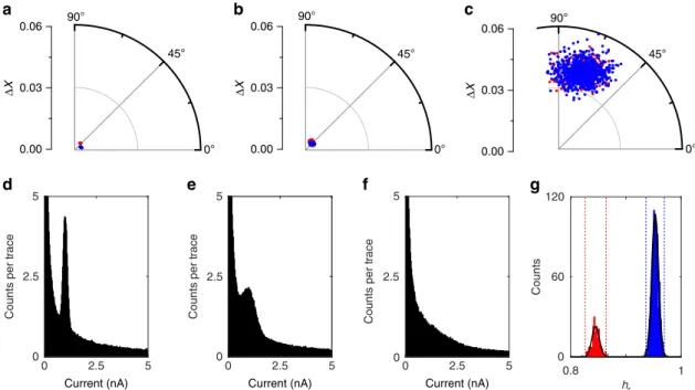
With regards to the effect of current noise, three data sets with different noise levels were generated,cf.Methods section. Briefly, each data set consisted of 1,000 I(s) traces, 80% of which were plain exponential decays (blue data points in Fig. 2) and 20% contained plateaus (Ip¼1 nA, red data points; the reference vector R was calculated using I(s)¼I0exp(bs) with b¼1 Å1, I0 20 nA (Note: the effect of the reference vector is demonstrated in Supplementary Fig. 1). A RoI was defined from 0.1 to 2 nm andDX,yandhrcalculated as described above. For comparison, we show the 1D all-data current histograms in Fig. 2d–f.
At low noise (10%Ips.d., STDEV), both MPVC and current-histogram-based methods show excellent performance: the polar plot clearly shows two distinct event clusters that can easily be separated based on DXand/or y (Fig. 2a). The all-data current histogram features a clear peak corresponding to Ip and the extraction of the molecular conductance is straightforward. At an intermediate noise level (30%Ip), some separation is still achieved in the polar plot (Fig. 2b), based on DX and y. The all-data current histogram displays a peak on top of an exponentially decaying background; its position can be found by appropriate data fitting.
Counts 0.8 1 0 60 120 hr a b c d e f g 0° 45° 90° 0° 45° 90° 0° 45° 90° 0.00 0.03 0.06 Δ X Counts p er trace 0 5 0 2.5 5 2.5 Current (nA) 0.00 0.03 0.06 Δ X 0.00 0.03 0.06 Δ X Counts p er trace 0 5 0 2.5 5 2.5 Current (nA) Counts p er trace 0 5 0 2.5 5 2.5 Current (nA)
Figure 2 | Simulated data with different noise levels.(a–c): Polar plots of data sets with increasing noise levels (10%, 30% and 100% STDEV, relative to theIp(1 nA), respectively). Blue cluster: exponentially decaying, featurelessI(s) traces; red cluster: plateau-containing traces. (d–f): All the data 1D current histograms (bin width: 0.025 nA). (g)hr-histogram of data set with 100% STDEV (bin width: 0.002).
However, at high noise (100%Ip), the two event clusters completely overlap in the (DX, y) plane of the cylindrical plot (Fig. 2c) and the peak feature in the histogram (Fig. 2f) is no longer visible. However, two distinct peaks emerge between 0.8 and 1 in thehr-histogram, as a third level of differentiation, and separation is still possible via MPVC, Fig. 2g (misclassification rate: 0%). The effect of multiple molecules bridging the gap at different noise levels is investigated in Supplementary Fig. 2. Consideration on the number of clusters is included in the Supplementary Figs 3–5. 2D current histograms and sample I(s) traces for each noise level are included in Supplementary Figs 6 and 7.
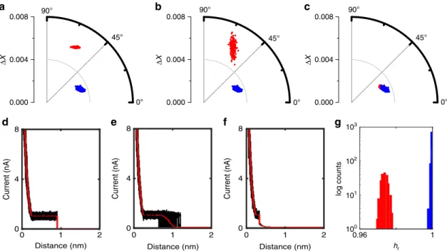
Next, we explored the effect of changes in the break-off distancesbas well as the effect of its variance, Fig. 3. As described above, those two factors are of special interest inI(s) experiments, because there is generally more than one possible way for a molecule to couple to the surface of electrodes13. As a result, differentsbvalues may be observed for a given molecular system, potentially also affecting the junction conductance (vide infra). As mentioned above, three simulated data sets were generated, cf. Methods section. Each data set consisted of 1000I(s) traces, 20% of which contained plateaus with break-off distances of sb¼0.9 nm, 0.9±0.1 nm and 0.35 nm, respectively (noise STDEV: 0.1 nA, RoI: 0.1 to 2 nm; red data points in Fig. 3). The remaining 80% were plain exponential decays (blue). 1D, 2D histograms and sample traces are included in Supplementary Figs 8 and 9.
ForI(s) traces with long plateaus (sb¼0.9 nm), Fig. 3a,b, the
two event classes appear as distinct clusters in the polar plot and separation is trivial (either based on DX or y). Under these conditions, a 1D current histogram also provides the plateau currentIpand hence the molecular conductance,cf. Supplementary Fig. 9. Once we allow for some variation around the mean break-off distance (0.9±0.1 nm), Fig. 3b,e, the plateau-containing cluster spreads out, in terms of bothDXandy, but is still well-separated from the exponential traces in the polar plot. On the other hand, in the 1D current histogram for shorter plateau lengths differentiation becomes increasingly difficult, and
essentially impossible for very short plateaus (sb¼0.35 nm), cf. Fig. 3c,f and Supplementary Fig. 9.
In the polar plot, the individual event clusters strongly overlap in theDX,ydimensions, but can be clearly differentiated viahr, as illustrated in Fig. 3g).
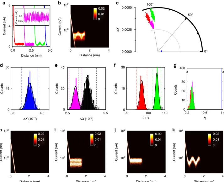
Subsequently, we investigated the ability of the vector-based method to differentiate sub-populations in the data. For this purpose, we generated 1000 I(s) traces of simulated data consisting of 40% exponential decays and 20% each of simple plateaus, and plateaus with superimposed sinusoidal and telegraphic noise features (additional current noise: 0.2 nA in all cases), Fig. 4a. While the exponential decays and plain plateaus stand for through-space tunnelling and conventional molecular bridging events (see above), the sine-shaped event is a proxy for non-linear event shapes, as reported previously12,23,22. Telegraphic noise features have also been observed previously
inI(s) experiments and are typically thought to be associated with
dynamic effects in the junction11,18,21. A polar plot showing the point density as well as the 1D current histogram are included in Supplementary Figs 10 and 11.
Such scenarios would normally be analysed using 2D current– distance histograms, since different event shapes become apparent, as long as the S/N ratio is sufficiently high. As shown in Fig. 4b, this is indeed the case, at least to some extent (note the logarithmic scale on the ordinate). However, without separating the individual traces, it would be difficult to extract the actual event characteristics or assess the relative abundance.
MPVC, on the other hand, does provide further insight into the individual event characteristics even at high low S/N levels, as shown in c (RoI 0.4–1 nm), and four event clusters become apparent (colour coding as in Fig. 4a). As mentioned above, we discuss the separation process in a sequential manner for illustration purposes.
First, theDXhistogram allows for differentiation between the exponential event cluster (blue, Fig. 4d), the telegraphic plateau cluster (magenta, Fig. 4e) and a third cluster, which encompasses the sine-shaped and plain plateau features (black, Fig. 4e). The latter is then differentiated in theyhistogram, as shown in panel
0° 45° 90° 0.000 0.004 0.008 Δ X 0° 45° 90° 0.000 0.004 0.008 0° 45° 90° 0.000 0.004 0.008 0.96 1 log counts hr Distance (nm) 0 1 2 Current (nA) 0 4 8 a b c g d e f Distance (nm) 0 1 2 Current (nA) 0 4 8 Distance (nm) 0 1 2 Current (nA) 0 4 8 100 101 102 103 Δ X Δ X
Figure 3 | Simulated data with varioussb.(a–c) Polar plots of data set withsbof 0.9 nm, 0.9±0.1 nm STDEV and 0.35 nm. (d–f) corresponding overlaid plots of plateau-containingI(s)traces (black) with their mean (red). (g)hrhistogram forsb¼0.35 nm data (bin width: 0.0014).
Fig. 4f. Further analysis of the data set via hr does not provide evidence for any further sub-populations, panel Fig. 4g, as expected for this simulated data set. Finally, we plot the 2D current histograms of each cluster, panels Fig. 4h–k. Each cluster is well separated and the individual event shapes can be identified. In addition, this analysis allows for the relative abundance of each event class to be determined, which would not be possible without some form of the data classification. In total, 3I(s)traces were mislabelled (0.3%), 20I(s)traces were outside the 2scutoffs used to define the individual event classes (2%).
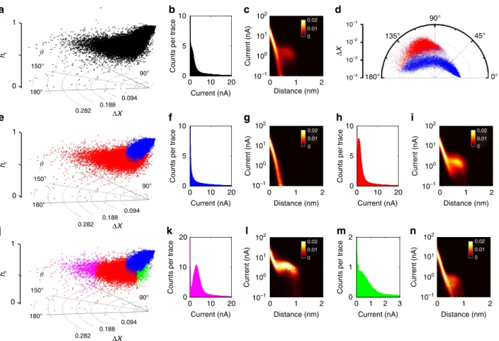
Experimental data. After testing the vector-based approach on simulated data, we apply the methodology to the experimental data, namely from experiments with Au/ODT/Au and Au/OPE/ Au. To this end, an extensive body of literature in both cases allows for an independent assessment of the results obtained here. For ODT, 70,000I(s)traces were recorded atVbias¼0.3 V and I0¼20 nA as described in the Methods section. (Note that this data set was previously published and analysed using a plateau identification algorithm which could however not discriminate
between different event classes12.) The RoI was from 0.25 to 2 nm (length of ODT, in an all-extended configuration: 1.52 nm, sb¼0.93 nm, accounting for tip-surface distance s0 at the set point current12).
DX, yand hrof the whole data set are visualized in cylinder coordinates in Fig. 5a. The all-data 1D and 2D log current histograms in Fig. 5b,c suggest the presence of plateau features, even though the S/N ratio in both representations is relatively low. Specifically, the 1D current histogram has a shoulder, that is a peak that is partially hidden in the exponential background, which could be analysed further using appropriate data fitting. The 2D log current–distance histogram reveals a faint plateau feature atIpE1 nA andsbE1 nm.
To explore the data further, the data set was clustered into two sub-clusters using a Gustafson–Kessel Fuzzy Clustering algo-rithm, a generalization of the fuzzyc-means algorithm (FCM)39, including covariance matrices that allows for the partitioning of ellipsoidal clusters (see Methods, Supplementary Note 1 and Supplementary Fig. 12 for limitations of cluster analysis)40. The ‘molecular’ data are contained in the red cluster (29,334 total). The blue cluster features the plain exponential traces without
Current (nA) 102 100 0 2 4 Distance (nm) 2.5 5.5 Counts 0 20 40 Current (nA) 102 100 0 2 4 Distance (nm) 3.5 4.5 Counts 0 15 30 ΔX (10–4) ΔX (10–3) Current (nA) 102 100 0 2 4 Distance (nm) 90 100 110 Counts 0 15 30 (°) Current (nA) 102 100 0 2 4 Distance (nm) Current (nA) 102 100 0 2 4 Distance (nm) a b c d h 2.5 0.0 5.0 0 4 8 Current (nA) Distance (nm) 0.25 0.5 Current (nA) f g 0.2 0.6 1.0 0 20 400 Counts hr e i j k 0° 50° 100° 0.0000 0.0025 0.0050 Δ X 10 30 0.02 0.01 0 0.02 0.01 0 0.02 0.01 0 0.02 0.01 0 0.02 0.01 0
Figure 4 | Vector-based analysis on different plateau shapes.(a) SimulatedI(s)traces with plain (red), telegraphic (magenta), sine-shaped (green) event features, as well as exponentially decaying traces (blue). Inset: enlarged section of telegraphic switching with dotted lines indicating the ‘on’ and ‘off’ states. (b) All-data 2D current histogram (Current binning: 150 bins/decade, distance bin width: 0.004 nm for all 2D histograms). (c) Polar plot of whole data set. (d)DX-histogram (bin width: 9107). (e)DX-histogram (bin width: 5105) Dashed lines represent 2scutoffs, grey bars indicate counts outside the cutoffs. (f)yhistogram (Bin width: 0.3°) (g)hrhistogram (Bin width: 8.5103) (h–k) 2D current histograms for each event cluster after separation.
plateaus (40,666 traces). A 2D log polar plot in Fig. 5c clearly shows the two distinct clusters emerging with the MPVC. In Fig. 5e, all three parameters are presented in a cylinder plot. Figure 5f,g shows the 1D and log 2D current histogram of the blue cluster, as expected, lacking any peaks or plateaus. The current histogram of the red cluster on the other hand features a clear peak at 1.0 nA corresponding toG¼3.3 nS (4.3105G0). This is close to the value previously reported for medium-conductance group in this system, with a most probable conductance of 3.82 nS (4.9105G0)13.
The identification of this conductance group raised the question, whether any other conductance groups, sometimes observed for ODT and other alkane dithiols depending on experimental conditions24,41–43, are also present in the data. For those groups, the most probable single-molecule conductance was reported to beG¼0.9 and 17 nS, respectively13. With the present choice of R, one would expect to find high-conductance traces towards higher DXas they would be further fromR, compared with the medium-conductance group. The low-conductance group should be closer to the reference vector and therefore should be found at low DX. As we show below, signatures of low- and high-conductance junctions are indeed found, even though they do not form distinct event clusters in the MPVC representation here (potentially due to low abundance).
To explore the low-conductance regime first, we selected the 5% of traces (1,467 total) within the red cluster that have the
lowestDX, as shown in green in Fig. 5j. (Note: in doing so this aspect can no longer be considered ‘unsupervised’, but this ‘sacrifice’ is accompanied by valuable additional insight into the data). Compiling these data into a 1D current histogram, Fig. 5m, yields a shoulder atIp¼0.4 nA (1.3 nS or 1.7105G0), which is indeed similar to the previously reported value for this group. However, the relatively lowIpvalue, its variance and the relatively low abundance of this group render its direct identification rather difficult. Figure 5n shows the corresponding 2D log current histogram.
A similar picture emerges for the junctions with high conductance. Again, we selected the 5% of molecular I(s)traces with the highest DX, Fig. 5j (magenta dots). The corresponding 1D current histogram, Fig. 5k, shows a peak at 3.15 nA (10.5 nS), which compares with 17 nS previously reported in the literature (2D log histogram shown in Fig. 5l). The reason for this discrepancy is currently unclear. However, closer inspection of the correspondingI(s) traces reveals that in our data, this group rarely entirely dominates an I(s) trace. Rather, we observed frequent switching between different conductance states within a given I(s) trace, which prevents the emergence of well-defined clusters in the MPVC representation and may lead to shifting of peaks in the 1D current histograms. Several examples are given in Supplementary Fig. 16, even though the statistical properties and physical reason behind this switching clearly require further study. Representative I(s) traces from predominantly
Current (nA) 0 10 20 Counts per trace 0 5 10 b Current (nA) 102 101 100 10–1 102 101 100 10–1 10–1 10–2 10–3 10–4 Distance (nm) 2 180° 135° 90° 45° 0° 0 1 c Current (nA) 0 10 20 Counts per trace 0 5 10 f Current (nA) Distance (nm) 2 0 1 g Current (nA) 0 10 20 Counts per trace 0 5 10 h Current (nA) 102 101 100 10–1 102 101 100 10–1 Distance (nm) 2 0 1 i Current (nA) 0 10 20 Counts per tr ace 0 10 20 k Current (nA) 102 101 100 10–1 Distance (nm) 2 0 1 l Current (nA) 0 1 2 Counts per tr ace 0 1 2 m 3 Current (nA) Distance (nm) 2 0 1 n a e Δ X d j hr 0 1 hr 0 1 hr 0 1 180° 90° 150° 0.094 0.188 0.282 180° 90° 150° 0.094 0.188 0.282 180° 90° 150° 0.094 0.188 0.282 ΔX ΔX ΔX 0.02 0.01 0 0.02 0.01 0 0.02 0.01 0 0.02 0.01 0 0.02 0.01 0
Figure 5 | Experimental data set of ODT.(a) Cylinder plot of all data points, (e) after Fuzzy Clustering and (j) with predominantly low (green, 5% lowest DX)/ high (magenta, 5% highestDX) conductance area indicated. (b,c) All the data 1D current and log 2D current–distance histogram. (d) LogDXcylinder plot, viewed alongzaxis, to illustrate the two clusters in the data set. (f,g) 1D current and log 2D current–distance histograms of exponential cluster. (h,i) 1D current and log 2D current–distance histograms of molecular cluster. (k,l) 1D current and log 2D current–distance histograms of high conductance cluster. (m,n) 1D current and log 2D current–distance histograms of low conductance region. (Bin widths: 0.1 nA for (b,f,h,k) and 0.015 nA for (m), Current binning: 150 bins/decade, distance bin width: 0.004 nm for all 2D histograms).
low, medium and high conductance region as well as a polar plot of the point density are provided in Supplementary Figs 13–15 (see also Supplementary Note 2).
The classification results above thus show that the algorithm is capable of identifying sub-populations in a large set of experimental I(s) traces, in the case of ODT, as well as their relative abundance. We did not observe distinct low- and high-conductance clusters in MPVC representation under the experi-mental conditions used. This may be due to low abundance or potentially suggest that distinct clusters do not form in these instances and the bottom and top 5% as defined above rather represent extreme values of a large distribution. Generally, good correspondence of conductance values with data previously reported in the literature, albeit recorded in many different experiments, further supports the applicability of this approach.
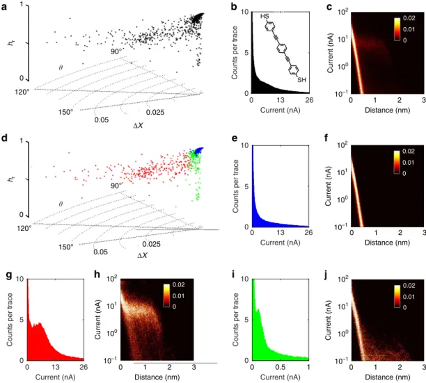
Finally, we applied the MPVC algorithm to OPE, Fig. 6b, inset44. Itsp-conjugated, rigid bridge motif has been studied in various forms in the context of single-molecule electronics over the last 20 years45. Although early reports presented conductance values over quite a broad range (102to 105 G0)46, in recent years several single-molecule studies of unfunctionalized OPE (for example, no solubilizing side groups) have converged on numbers between 1.2 to 2.9104 G0 (refs 44,46–51). An additional through-molecule conductance feature ato105G0is also sometimes observed (perhaps most clearly when the
molecule is functionalized with hexyloxy solubilizing groups)49,52,53. This has been attributed to conductance through two molecules of OPE interacting via p–p stacking52 between phenyl groups, a configuration first observed in monothiolated OPE-analogues by Wu et al.44. In support of this hypothesis, it is noted that the low-conductance feature exhibits a larger sb than the high-conductance plateau. To this end, we applied the above process to a data set consisting of 2,000 I(s)traces (RoI: 0.4 to 4 nm based on a sulfur–sulfur distance for this molecule of 2.07 nm (ref. 44).
DX,yand hrof the whole data set are shown in the cylinder plot in Fig. 6a. The corresponding plot of the point density is provided in Supplementary Fig. 17. Multiple populations become visible in this representation. Accordingly, there is a shoulder in the all data 1D current histogram (Fig. 6b) as well as the faint plateau in the 2D log current histogram (Fig. 6c). In contrast to ODT, OPE shows a lower junction formation probability, which renders the assignment of single-molecule conductance values from all-data representations more difficult and data classification even more important.
By clustering DX, y and hr of the whole data set with a Gustafson–Kessel Fuzzy Clustering algorithm, the data split up into three clusters (Supplementary Note 3). The blue sub-group consists only of featureless exponential decays, as confirmed by the 1D current and 2D log current–distance histograms
Current (nA) 0 13 26 Counts per trace 0 5 10 SH HS Current (nA) 0 13 26 Counts per trace 0 5 10 b e c Current (nA) 3 102 101 100 10–1 102 101 100 10–1 102 101 100 10–1 102 101 100 10–1 0 1 Distance (nm) 2 f 3 0 1 Distance (nm) 2 Current (nA) Current (nA) Counts p er tr ace 0 5 10 i 0 0.5 1 j Current (nA) 3 0 1 Distance (nm) 2 g Current (nA) 0 13 26 Counts p er tr ace 0 5 10 h Current (nA) 3 0 1 Distance (nm) 2 d a hr 0 1 hr 0 1 90° 90° 120° 120° 150° 150° 0.025 0.05 0.025 0.05 ΔX ΔX 0.02 0 0.02 0.01 0 0.02 0.01 0 0.02 0.01 0 0.02 0.01 0
Figure 6 | Experimental data set of OPE.(a,d) Cylinder plots of experimental data unassigned, and after Fuzzy Clustering. (b) All data 1D current histogram with OPE inset (bin width 0.1 nA). (c) All data 2D log current histogram. (e,f): 1D current (bin width 0.1 nA) and 2D log current histogram of the plain exponential cluster. (g,h) 1D current and 2D log current histograms of the high conductance cluster (bin width 0.1 nA). (i,j) 1D current (Bin width 0.005 nA) and 2D log current histogram of the low-conductance cluster (2D log histograms: 100 bins/decade, 1,000 bins/nm).
(Fig. 6e,f), lacking any peaks or plateaus. The cluster encompasses B74% of the total number ofI(s) traces.
The peak current of the red, high-conductance cluster (14% of total traces) was determined from the 1D current histogram in g) to be 5.5 nA (13.8 nS, 1.8104G0), as compared to the value of 9.3 nS (1.2104G0) reported previously46. The corresponding plateau can be seen clearly in the 2D log current histogram in Fig. 6h. The colour-coded cylinder plot in Fig. 6d shows the position of each cluster.
Extracted from the green cluster in I (11% of total traces), the 1D current histogram features a low-conductance group with a current maximum at 0.11 nA, corresponding to 0.28 nS
(3.6106 G0). This compares with the ‘two-molecule’
conductance case reported by Calame et al. with 0.46 nS (ref. 44; 5.9106 G0), where the occurrence of the low conductance group is explained by aromatic (p/p) coupling between two molecules. Interestingly, the peak feature in i) results from a rather small number of traces (22 or 1% or the overall data set) with hro0.6, as shown in Supplementary Fig. 21 (a small sub-cluster in the green data points can also be seen in Fig. 6d), towards lowhrvalues). As shown in Supplementary Fig. 22, this small sub-cluster features an apparent break-off distance of 2.6 nm (sbhistogram shown in Supplementary Fig. 21). Account-ing for the length of the gold–thiol bonds and s0, this yields a sulfur–sulfur distance of 2.7 nm, which is in very good agreement with the value of 2.91 nm, as reported by Calameet al.
The remainder of the data in the green cluster (B200 traces, 10%) appear to show a plateau-like feature, which is, however, relatively poorly defined. sb isB0.7 nm, much shorter than the (extended) molecular length of 2.07 nm, vide supra. It is thus possible that those traces originate from junctions where the tip makes contact to the molecule in an ‘off centred’ configuration, that is the molecular bridge ruptures well before the tip/surface distance reaches the molecular length. Sample traces of both high-and low-conductance class are provided in Supplementary Figs 18 and 19 together withhrand 2D log current histograms of the low conductance cluster in Supplementary Figs 20–23.
As previously observed for the simulated as well as the ODT data, we were able to identify the most abundant feature in the data set with good agreement to previously reported values forG
andsb. We also found specific, previously known sub-groups and
were able to extract their relative abundance, information that would normally be inaccessible with conventional methods of analysis.
Discussion
We have demonstrated here that multivariate pattern analysis, in particular MPVC, is a powerful tool for analysing single-conductance data. In contrast to conventional current- or current–distance histogram-based analysis, MPVC does not make any prior assumptions with regards to the shape of a molecular signature in theI(s) trace, or their relative statistical abundance in the data set. Rather, the algorithm looks for similarity between data sets, in terms of vector distance, angle and (reduced) Hamming distance, relative to a common reference. The latter allows one to focus on particular event characteristics, if required, and reduces the complexity of the data significantly.
In the simulated data that closely resemble experimentalI(s) traces, we illustrate the general effect of different molecular characteristics on the classification parameters, such as the statistical variation in the plateau current Ip or the break-off distancesb. Some of these result in distinct cluster shapes, which may facilitate an initial assessment of the junction characteristics. More detailed analysis allows for extraction of different event classes as well as their relative abundance, which are inaccessible
with conventional methods of analysis, in particular for very large data sets.
Furthermore, we employed MPVC to two experimental systems with up to 70,000 I(s) traces, namely Au/Au junctions of ODT and OPE, as well-characterized model systems. In both cases, we confirmed the single-molecule conductance values and break-off distances reported in the literature, notably in one data set and without hand selection of the data. We also found sub-populations in the data that would be invisible to all-data analyses, and were able to propose a link to their physical origin (for example,p/pstacking interaction between OPE dimers).
More generally, the present study highlights the potential of machine learning algorithms in single-molecule science, which may provide new insight into physical processes at the nanoscale, in device or sensing applications.
Methods
Simulated Data.The simulated data was generated in MATLAB (2015a) to correspond to experimentalI(s)data recorded at a bias voltage of 0.3 V and at a
I0of 20 nA12. Data sets contained 1,000 individualI(s)traces. Two thousand data
points were produced per individual model trace at a distance between 0 and 4 nm. From experimental data, the most probable exponential decay coefficient was determined to be 1.2 Å1, which was used for the simulated data12.
The simulated data was created with a plateau currentIpof 1 nA (Fig. 2, Fig. 3),
0.5 nA (Fig. 4) and break-off pointssbat 0.9 nm (Fig. 2) and 1.5 nm (Fig. 4).
STDEVs forIpandsbwere added by generating a random number with a certain
STDEV around 0 and adding it to the initial value. Noise was introduced by pairwise multiplying a random vector which was distributed around 1 with a given STDEV, with the initial noise-free model vector. Data for Fig. 3 was generated with a noise STDEV of 0.1 nA. Data for Fig. 4 was generated with 0.2 nA noise STDEV,
IpSTDEV 0.025 andsbSTDEV 0.05 nm. Telegraphic plateaus in Fig. 4 were
generated by randomly switching points in the plateau betweenIpand 0.5Ip. The
sine-shaped plateauI(s)traces were generated by adding a sine wave with amplitude 0.2 nA and a cycle period of 0.66 nm to the plateau.
Experimental Data.TheI(s) data sets for ODT used in the present analysis were previously published by Inkpenet al., with new data for OPE collected using an identical experimental method12. OPE was prepared by Sonogashira cross-coupling
of 4-iodophenylthioacetate and 1,4-diethynylbenzene54. Sub-monolayers of OPE
on Au were formed by immersion of the single-crystal substrate into a 0.01 mM solution of the freshly deacetylated compound in THF for 45 s. Deacetylation was facilitated by the addition of 1ml NH4OH per 1 ml analyte solution followed by
incubation for 10–15 min at room temperature45,54. Compared with previously reported experiments using ODT, OPE provided lower and more variable JFPs (typicallyB4% based on data selection using an objective algorithm12where
BW¼0.1, 0.2, 0.3, 0.4; PDBC450). Two thousandI(s)traces were recorded at 26 nAI0and 0.4 V.
MPVC.Simulated and experimental data sets were analysed with the vector-based classification approach as described in the main text. For the analysis a noise-free reference vector was used (I0¼20 nA for ODT and 26 nA for OPE, decay
coeffi-cientb¼1.0 Å1), cf. Supplementary Note 4. The data set and reference were divided by the scanner range (100 nA) multiplied by the square root of the number of data points in the region of interest to normalize,cf. equation (1). This ensured that the maximal possible separation between points was unity.sbwas calculated by
taking 3sof the distribution of the last 1 nm of the individualI(s)traces as a threshold.sbwas considered the distance of the first current value below this
threshold starting from the beginning of the trace. Fuzzy Clustering was performed with the ‘Clustering and Data Analysis Toolbox’ by J. Abonyiet al.downloaded from MATLAB file exchange.
Computer code availability.All relevant scripts are available from the authors on request.
Data availability.All relevant data are available from the authors on request.
References
1. Park, H., Lim, A. K. L., Alivisatos, A. P., Park, J. & McEuen, P. L. Fabrication of metallic electrodes with nanometer separation by electromigration.Appl. Phys. Lett.75,301–303 (1999).
2. Reed, M. A., Zhou, C., Muller, C. J., Burgin, T. P. & Tour, J. M. Conductance of a molecular junction.Science278,252–254 (1997).
3. Xu, B. & Tao, N. Measurement of single-molecule resistance by repeated formation of molecular junctions.Science301,1221–1223 (2003).
4. Haiss, W.et al.Measurement of single molecule conductivity using the sponta-neous formation of molecular wires.Phys. Chem. Chem. Phys.6,4330–4337 (2004).
5. Rubio, G., Agraı¨t, N. & Vieira, S. Atomic-sized metallic contacts: mechanical properties and electronic transport.Phys. Rev. Lett.76,2302–2305 (1996). 6. Ivanov, A. P.et al.DNA tunneling detector embedded in a nanopore.Nano
Lett.11,279–285 (2011).
7. Ivanov, A. P., Freedman, K. J., Kim, M. J., Albrecht, T. & Edel, J. B. High precision fabrication and positioning of nanoelectrodes in a nanopore.ACS Nano8,1940–1948 (2014).
8. Albrecht, T., Guckian, A., Ulstrup, J. & Vos, J. G. Transistor-like Behavior of Transition Metal Complexes.Nano Lett.5,1451–1455 (2005).
9. Albrecht, T., Guckian, A., Kuznetsov, A. M., Vos, J. G. & Ulstrup, J. Mechanism of electrochemical charge transport in individual transition metal complexes.
J. Am. Chem. Soc.128,17132–17138 (2006).
10. Albrecht, T.et al.Scanning tunneling spectroscopy in an ionic liquid.J. Am. Chem. Soc.128,6574–6575 (2006).
11. Albrecht, T., Mertens, S. F. L. & Ulstrup, J. Intrinsic multistate switching of gold clusters through electrochemical gating.J. Am. Chem. Soc.129,9162–9167 (2007). 12. Inkpen, M. S.et al.New insights into single-molecule junctions using a robust, unsupervised approach to data collection and analysis.J. Am. Chem. Soc.137,
9971–9981 (2015).
13. Nichols, R. J.et al.The experimental determination of the conductance of single molecules.Phys. Chem. Chem. Phys.12,2801–2815 (2010). 14. Gamow, G. Zur quantentheorie des atomkernes.Zeitschrift fu¨r Phys51,
204–212 (1928).
15. Williams, P. D. & Reuter, M. G. Level alignments and coupling strengths in conductance histograms: the information content of a single channel peak.J. Phys. Chem. C117,5937–5942 (2013).
16. Jang, S. Y., Reddy, P., Majumdar, A. & Segalman, R. A. Interpretation of stochastic events in single molecule conductance measurements.Nano Lett.6,
2362–2367 (2006).
17. Quan, R., Pitler, C. S., Ratner, M. A. & Reuter, M. G. Quantitative
interpretations of break junction conductance histograms in molecular electron transport.ACS Nano9,7704–7713 (2015).
18. Albrecht, T. Electrochemical tunnelling sensors and their potential applications.
Nat. Commun3,829 (2012).
19. Yoshida, K.et al.Correlation of breaking forces, conductances and geometries of molecular junctions.Sci. Rep5,9002 (2015).
20. Kihira, Y., Shimada, T., Matsuo, Y., Nakamura, E. & Hasegawa, T. Random telegraphic conductance fluctuation at Au-pentacene-Au nanojunctions.Nano Lett.9,1442–1446 (2009).
21. Adak, O.et al.Flicker noise as a probe of electronic interaction at metal-single molecule interfaces.Nano Lett.15,4143–4149 (2015).
22. Su, T. A., Li, H., Steigerwald, M. L., Venkataraman, L. & Nuckolls, C. Stereo-electronic switching in single-molecule junctions.Nat. Chem7,215–220 (2015). 23. Fujihira, M., Suzuki, M., Fujii, S. & Nishikawa, A. Currents through single
molecular junction of Au/hexanedithiolate/Au measured by repeated formation of break junction in STM under UHV: effects of conformational change in an alkylene chain from gauche to trans and binding sites of thiolates on gold.Phys. Chem. Chem. Phys.8,3876–3884 (2006).
24. Li, C.et al.Charge transport in single Au / Alkanedithiol / Au junctions: coordination geometries and conformational degrees of freedom.J. Am. Chem. Soc.130,318–326 (2008).
25. Kiguchi, M.et al.Single molecular resistive switch obtained via sliding multiple anchoring points and varying effective wire length.J. Am. Chem. Soc.136,
7327–7332 (2014).
26. Ulrich, J.et al.Variability of conductance in molecular junctions.J. Phys. Chem. B110,2462–2466 (2006).
27. Venkataraman, L., Klare, J. E., Nuckolls, C., Hybertsen, M. S. & Steigerwald, M. L. Dependence of single-molecule junction conductance on molecular conformation.
Nature442,904–907 (2006).
28. Reuter, M. G., Hersam, M. C., Seideman, T. & Ratner, M. A. Signatures of cooperative effects and transport mechanisms in conductance histograms.
Nano Lett.12,2243–2248 (2012).
29. Tao, N. J. Electron transport in molecular junctions.Nat. Nanotechnol1,
173–181 (2006).
30. Krstic, P., Ashcroft, B. & Lindsay, S. Physical model for recognition tunneling.
Nanotechnology26,84001 (2015).
31. Chang, S.et al.Chemical recognition and binding kinetics in a functionalized tunnel junction.Nanotechnology23,235101 (2012).
32. Haxby, J. V., Connolly, A. C. & Guntupalli, J. S. Decoding neural representational spaces using multivariate pattern analysis.Annu. Rev. Neurosci.435–456 (2014).
33. Naselaris, T., Kay, K. N., Nishimoto, S. & Gallant, J. L. Encoding and decoding in fMRI.Neuroimage56,400–410 (2011).
34. Hamming, R. W. Error detecting and error correcting codes.Bell Syst. Tech. J. XXIX,147–160 (1950).
35. Rodriguez, A. & Laio, A. Clustering by fast search and find of density peaks.
Science344,1492–1496 (2014).
36. MacQueen, J. B. inProceedings of 5th Berkeley Symposium on Mathematical Statistics and Probability281–297 (Berkeley, CA, USA, 1967).
37. Kaufman, L. & Rousseeuw, P. J. Clustering by means of medoids. inStatistical Data Analysis: Based on the L1-Norm and Related Methods. First International Conference1–12 (1987).
38. Gustafson, D. E. & Kessel, W. C. in1978 IEEE Conference on Decision and Control including the 17th Symposium on Adaptive Processes761–766 (San Diego, CA, USA, 1978).
39. Yang, M. S. A survey of fuzzy clustering.Math. Comput. Model18,1–16 (1993). 40. Ho¨ppner, F., Klawonn, F., Kruse, R. & Runkler, T.Fuzzy Cluster Analysis
(Wiley, 1999).
41. Haiss, W.et al.Impact of junction formation method and surface roughness on single molecule conductance.J. Phys. Chem. C113,5823–5833 (2009). 42. Li, X.et al.Conductance of single alkanedithiols: conduction mechanism and effect
of molecule - electrode contacts.J. Am. Chem. Soc.128,2135–2141 (2006). 43. Frei, M., Aradhya, S. V., Hybertsen, M. S. & Venkataraman, L. Linker
dependent bond rupture force measurements in single-molecule junctions.J. Am. Chem. Soc.134,4003–4006 (2012).
44. Wu, S.et al.Molecular junctions based on aromatic coupling.Nat. Nanotechnol.3,569–574 (2008).
45. Tour, J. M.et al.Self-assembled monolayers and multilayers of conjugated thiols,a,o-dithiols, and thioacetyl-containing adsorbates. understanding attachments between potential molecular wires and gold surfaces.J. Am. Chem. Soc.117,9529–9534 (1995).
46. Huber, R.et al.Electrical conductance of conjugated oligomers at the single molecule level.J. Am. Chem. Soc.130,1080–1084 (2008).
47. Xiao, X., Nagahara, L. A., Rawlett, A. M. & Tao, N. Electrochemical gate-controlled conductance of single oligo (phenylene ethynylene) s.J. Am. Chem. Soc.127,9235–9240 (2005).
48. Xing, Y.et al.Optimizing single-molecule conductivity of conjugated organic oligomers with carbodithioate linkers.J. Am. Chem. Soc.132,7946–7956 (2010). 49. Kaliginedi, V.et al.Correlations between molecular structure and single
junction conductance: a case study with oligo(phenylene-ethynylene)-type wires.J. Am. Chem. Soc.134,5262–5275 (2012).
50. Kolivoska, V.et al.Electron transport through catechol-functionalized molecular rods.Electrochim. Acta110,709–717 (2013).
51. Frisenda, R., Perrin, M. L., Valkenier, H., Hummelen, J. C. & Van der Zant, H. S. J. Statistical analysis of single-molecule breaking traces.Phys. Status Solidi B250,
2431–2436 (2013).
52. Gonzalez, M. T.et al.Break-junction experiments on acetyl-protected conjugated dithiols under different environmental conditions.J. Phys. Chem. C 115,17973–17978 (2011).
53. Martin, S.et al.Identifying diversity in nanoscale electrical break junctions.J. Am. Chem. Soc.132,9157–9164 (2010).
54. Liu, K., Wang, X. & Wang, F. Probing charge transport of ruthenium-complex-based molecular wires at the single-molecule level.ACS Nano2,2315–2323 (2008).
Acknowledgements
The authors would like to thank The Leverhulme Trust (M.L., M.S.I., N.J.L., T.A.) and the Wellcome Trust (K.K.) for funding.
Author contributions
All the authors contributed to the writing of the article and interpretation of the results.
Additional information
Supplementary Informationaccompanies this paper at http://www.nature.com/ naturecommunications
Competing financial interests:The authors declare no competing financial interests.
Reprints and permissioninformation is available online at http://npg.nature.com/ reprintsandpermissions/
How to cite this article:Lemmer, M.et al.Unsupervised vector-based classification of single-molecule charge transport data.Nat. Commun.7,12922 doi: 10.1038/ncomms12922 (2016).
This work is licensed under a Creative Commons Attribution 4.0 International License. The images or other third party material in this article are included in the article’s Creative Commons license, unless indicated otherwise in the credit line; if the material is not included under the Creative Commons license, users will need to obtain permission from the license holder to reproduce the material. To view a copy of this license, visit http://creativecommons.org/licenses/by/4.0/