Multiagent Coordination for Energy Consumption Scheduling in Consumer Cooperatives

Multiagent Coordination for Energy Consumption Scheduling in Consumer

Cooperatives

Andreas Veit

Ying Xu

Ronghuo Zheng

Nilanjan Chakraborty

Katia Sycara

Karlsruhe, Germany Pittsburgh, PA 15213 Pittsburgh, PA 15213

[email protected] {yingx1, ronghuoz}@andrew.cmu.edu {nilanjan, katia}@cs.cmu.edu

Abstract

A key challenge to create a sustainable and energy-efficient society is in making consumer demand adap-tive to energy supply, especially renewable supply. In this paper, we propose a partially-centralized organiza-tion of consumers, namely, a consumer cooperative for purchasing electricity from the market. We propose a novel multiagent coordination algorithm to shape the energy consumption of the cooperative. In the cooper-ative, a central coordinator buys the electricity for the whole group and consumers make their own consump-tion decisions based on their private consumpconsump-tion straints and preferences. To coordinate individual con-sumers under incomplete information, we propose an iterative algorithm in which a virtual price signal is sent by the coordinator to induce consumers to shift demand. We prove that our algorithm converges to the central op-timal solution. Additionally we analyze the convergence rate of the algorithm via simulations on randomly gen-erated instances. The results indicate scalability with re-spect to the number of agents and consumption slots.

Introduction

A key challenge in creating an energy-efficient society is to adapt electricity demand to supply conditions, e.g., by re-ducing peak electricity demand. The energy demand man-agement becomes more critical when the energy supply un-certainty rises as is the case with increasing penetration of renewable energy in the electricity market (Medina, Muller, and Roytelman 2010a). A straightforward way to manage consumer demand is via direct load control (DLC), in which utility companies directly control the power consumption of consumers’ appliances by switching them on/off. In small scale pilot studies, DLC has been successful in reducing peak energy consumption by better matching of supply and demand. However, the biggest drawback of DLC is that con-sumers may not be comfortable with utility companies hav-ing direct control over their appliances (Rahimi and Ipakchi 2010; Medina, Muller, and Roytelman 2010b). An indi-rect method of controlling the overall demand is to use tar-iffs (such as time-of-use (TOU) pricing) to incentivize con-sumers to shift peak time energy use. Recent technological

Copyright c2013, Association for the Advancement of Artificial Intelligence (www.aaai.org). All rights reserved.

advances in smart meters and smart appliances, have en-abled direct and real time participation (RTP) of an individ-ual consumer in the energy market through the use of soft-ware agents. A key feature of RTP programs is that each cus-tomer communicates with the utility companies individually which may lead to undesirable effects like herding (Ram-churn et al. 2012).

In (Mohsenian-Rad et al. 2010) it is argued that a good demand side management program should focus on control-ling the aggregate load (which is also important for eco-nomic load dispatching (Wood and Wollenberg 1996)) of a group of consumers instead of individual consumers. There-fore, in this paper we introduce and study the problem of coordinating a group of consumers called consumer coop-eratives. A consumer cooperative allowspartial centraliza-tionof consumers represented by a group coordinator (me-diator) agent, who purchases electricity from utilities or the market on their behalf. Such consumer configurations can potentially increase energy efficiency via aggregation of de-mand to reduce peak power consumption, and direct partici-pation in the energy markets. The coordinator is not a market maker or a traditional demand response aggregator (Jellings and Chamberlin 1993) since it neither sets energy prices nor aims to incur profits by selling to the market. Rather, its role is akin to a social planner’s in that it manages the demand of its associated consumer group for cost effective electricity allocation. It has to ensure that the demand goals and con-straints of group members (consumers) are fulfilled, while also helping flatten out peak demands for the group. The consumers espouse the goals of the group, however they are not willing to totally disclose their demand goals and con-straints to either other firms or the coordinator. Moreover, the members autonomously decide how to shift their loads to help the group flatten peak demands. Real world consumer groups coordinated in the above manner can be formed natu-rally in many application scenarios, especially when they are geographically co-located, e.g., industrial parks/technology parks, commercial estates, large residential complexes.

The partially centralized coordination model offers sev-eral advantages to the stakeholders. For individual con-sumers, participation in such energy groups allows them to retain control of their own appliances. In addition, the con-sumers can obtain electricity at better prices than they would have obtained if they bought individually. The price

advan-tage is due to three reasons. First, because of its size, the me-diated participation of the consumer group in the market al-lows the group to enter into more flexible purchase contracts. This has the result that the price paid by the consumers re-flect more accurately the actual cost of production (which is not the case in current long term fixed contract struc-tures (Kirschen 2003)). Second, by buying as a collective, the group can benefit from volume discounts. The situation here is analogous to group insurance programs in compa-nies. Third, in negotiated electricity contracts, the price usu-ally consists of two components, one coming from the actual energy production cost and the other as a premium against volatility in the energy demand and/or supply. Buying as a group helps in reducing the premium against volatility since the coordinated demand management can achieve higher stability of demand and reduce demand peaks. From the util-ity’s perspective, the consumer groups are large enough to be useful in demand response programs and have more pre-dictable demand shifts compared to individual consumers.

The technical challenge in designing a consumer cooper-ative is that the central coordinator does not know the con-straints of the individual consumers and thus cannot com-pute the optimal demand schedule on its own. Furthermore, the actual cost of electricity consumption will depend on the aggregate consumption profile of all agents and the agents may not want to share their consumption patterns or con-sumption constraints with other agents. Therefore, in this pa-per, we design an algorithm that enables the central agent to coordinate the consumers to achieve the optimal centralized consumption load where the agents have private knowledge about their consumption constraints.

We design an iterative algorithm where, in each iteration, the coordinator sends avirtual price signalto the consumers and the agents compute their consumption profiles based on this price signal and send it back to the coordinator. We prove that this iterative algorithm ensures that the agents converge to the optimal centralized schedule. This provably optimal demand scheduling algorithm for consumer cooper-atives is the primary contribution of this paper.

Related Work

Demand response programs for managing consumer side de-mand have been studied from a variety of directions ranging from direct load control to indirect incentive based control (please see (Medina, Muller, and Roytelman 2010a) and ref-erences therein for an overview). Here, we will restrict our discussion to demand management using variable price sig-nal as this is most relevant to our current work.

In the extant literature on indirect demand shaping it is (implicitly or explicitly) assumed that the utility companies can send a price signal to software agents at the smart me-ters that respond to this price and schedule the appliances for the future (examples include (Philpott and Pettersen 2006; Chu and Jong 2008; Parvania and Fotuhi-Firuzabad 2010; Pedrasa, Spooner, and MacGill 2010; Conejo, Morales, and Baringo 2010; Kim and Poor 2011; Tanaka et al. 2011; Dietrich et al. 2012; Roozbehani et al. 2012; Mohsenian-Rad and Leon-Garcia 2010)). However, with such price sig-nals, in theory, there is a possibility of instabilities like

herd-ing phenomenon, whereby agents move their consumptions towards the low price times and thus cause a spike in de-mand, thereby increasing the energy cost. Various heuristics have been proposed, but there is no algorithm with prov-able guarantees to solve this problem (Ramchurn et al. 2012; Voice et al. 2011; Ramchurn et al. 2011). A key feature of this work is that the agents communicate directly with the utilities and the focus is on controlling the overall load by interacting directly with each consumer. There is no interac-tion among the consumers.

In contrast, (Mohsenian-Rad et al. 2010) have focused on a utility or a generator controlling the load of a group of con-sumers. The authors accomplish this by allowing the indi-vidual consumers to interact with one another. The problem is formulated in a game-theoretic framework and the con-sumers coordinate in an iterative manner and exchange their demand profiles (but not their consumption constraints with each other). In this paper, we consider consumers interact-ing as a group with the utility, but our consumer architecture is different. We assume the consumers to form a cooperative with a central coordinator and our agents do not share their consumption profiles with other agents.

Problem Formulation

We consider a central coordinator purchasing electricity from the electricity market to support demands of a con-sumer group. We assume that the price is known over the whole planning horizon. This is true when the agent group has a long term electricity contract (say yearly) and the agents planning horizon is shorter (say1day). The contract is not a flat rate contract since in this case there would be no economic incentive for the agents to shift their demands.

We consider N members in a group with the planning period divided into M discrete time slots. The number of discrete time slots we consider is dependent on the market price structure, which can be different in practice based on the utility companies. For example,M = 2for time-of-use pricing with different prices during day and night, whereas

M = 24in an hourly pricing scheme. LetRbe anN×M

matrix where each row of the matrix, ri is the electricity demand of the agent i,i ∈ {1,2, . . . , N}. We callri the demand profileof agent i. Each entryrij is the electricity demand of agentifor time slotj. The total aggregated de-mand in time slotj isρj =P

N

i=1rij. The average market price of a unit electricity at time slotjis defined asp_j(ρj).

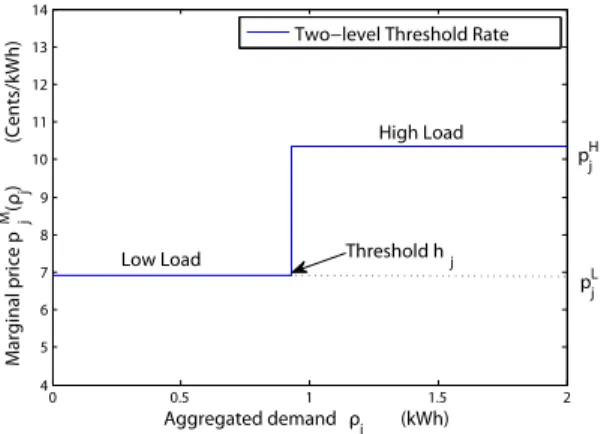
We assume a typical market price function where the prices are different in each time slot and has a threshold structure. For each time slot, every unit of electricity con-sumed below a specified threshold is charged at a lower price, while any additional unit exceeding that threshold is charged at a higher price. Thus, the marginal electricity price in a time slot, denoted bypM

j (ρj), is a non-decreasing func-tion of the total demand. The marginal price at a given de-mand is payment increment (decrement) for adding (reduc-ing) one unit of electricity. Figure (1) shows an example for a two level threshold price function adopted from BC Hydro.1

The marginal price of a two-level threshold structure can 1

0 0.5 1 1.5 2 4 5 6 7 8 9 10 11 12 13 14 Aggregated demand ρ_j (kWh) Marginal price p j M(ρ j ) (Cents/kWh)

Two−level Threshold Rate

High Load

Threshold h_j

Low Load

p_jH

p_jL

Figure 1: Two-level Threshold Pricing Rates by BC Hydro.

formally be written as follows:pM j (ρj) = _pH j ρj> hj pL j ρj≤hj with pH

j > pLj, where hj is the threshold for consump-tion in time slot j. We further assume that the high price in any time slot is greater than the low price in any other time slot, i.e.,pH

j > pLk, ∀j, k. Letx

+ _{= max{0, x}and}

x−= min{0, x}. The energy cost for time slotjis thus:

pj(ρj)ρj =pHj ρ0j−hj +

+pLj ρ0j−hj −

+pLjhj (1)

The demand profile of each agent ri must satisfy their individual constraints. We assume that the total demand of each agent during the whole planning period is fixed, i.e., PM

j=1rij =τi, whereτiis the total demand for agenti. The overall demand can come from two types of loads, shiftable loads and non-shiftable loads. We will consider loads where the consumption constraints are given by a constraint setXi which is private knowledge of the agenti. An agent does not share this constraint setXi, neither with other firms nor with the coordinator. Unless otherwise specified we will as-sume that Xi can be expressed by constraints of the form

rij ∈[rij, rij]specifying the minimum and maximum con-sumption of agentiin time slotj, whererij ≥0. Note that these constraints are linear andXiis a convex polytope. In some application scenarios, when an agent determines its en-ergy consumption profile, it has to consider additional cost associated with the consumption schedule. For example in a factory the energy is usually for production. Thus changing the energy consumption schedule may mean changing the production process, thereby, the production cost. For agent

i, we denote this cost byg_i(ri). We assume this cost func-tion to be convex. The overall cost funcfunc-tion of each agent is thenPM

j=1pj(ρj)rij+ gi(ri). With the objective to mini-mize the sum of all agents costs, thecentral energy alloca-tion problemcan be written as:

min C (R) := PN i=1 PM j=1pj(ρj)rij+P N i=1gi(ri) s.t. ri∈ Xi, P M j=1rij =τi. (2) where the energy allocationsrij are the optimization vari-ables. Note that the above problem is defined on a convex set

Xi. Although the objective function is non-linear it is convex because of the following. First,PN

i=1 PM

j=1pj(ρj)rij = PM

j=1pj(ρj)ρjis convex and non-decreasing inρjas indi-cated by Equation (1). Together withρj=P

N

i=1rij, we can conclude thatPM

j=1pj(ρj)ρjis convex inrij,∀i, j(Boyd and Vandenberghe 2004). Sinceg_i(ri)is also convex, the to-tal cost functionC (R)is a summation of convex functions and so also convex. Thus Problem (2) is a convex minimiza-tion problem.

Solution Approach

Although the problem in (2) is a convex optimization prob-lem, since the constraints and preferences of the agents are private knowledge, the consumption profiles cannot be com-puted directly by the central coordinator. Since the con-straints in Problem (2) are agent-specific, they are naturally separable. The objective function, although a sum of the in-dividual costs of each agent, is coupled, because the price of electricity in any time slot,j, depends on the aggregated consumption of all agents ρj. Therefore, we use a primal decomposition approach to solve the problem in which the sub-problems correspond to each agent optimizing its own energy cost subject to their individual constraints. The cen-tral coordinator has to compute the appropriate information to be sent to the agents so as to guide the consumption pat-tern towards time slots with lower prices (this corresponds to the master problem in primal decomposition methods).

An intuitive solution approach would be for the coordina-tor to tell the agents the aggregated demand in each time slot. Knowing the market price, the agents could then solve their individual optimization problems. This approach has prob-lems because the agents don’t know the constraints and con-sumption preferences of the other agents in the group, while their costs strongly depend on the consumption of the other agents. For example all agents knowing the market price and the current aggregated demand could shift as much demand as possible to a supposedly cheap time slot. This would lead to a herding phenomenon, where all agents would move to the cheap time slot resulting in a rise in the demand and thus increasing the total cost. This effect is shown in Figure (2) where part (a) illustrates an initial setting before the shift and part (b) shows a demand profile resulting from the herding phenomenon. Thus, the key challenge is to design the price signal which the coordinator sends to the agents.

We propose a novel virtual price signal that the coordina-tor uses to guide the agents’ demand profiles. A virtual price signal is not the final price the agents have to pay, but infor-mation about what they would have to pay, given the current aggregated demand. The goal of designing the virtual price signal is to enable the agents to foresee the possible price in-crement/reduction caused by their demand shifting. There-fore, the virtual price signal, sij(rij), is a function of the agents demand in each time slot. To design the virtual price signal the coordinator first computes the amount of demand that should be ideally shifted in each time slot. As shown in Figure (2a), this amount, denoted by∆j,j = 1,2,3, is the difference between the total demand and the threshold

1 2 3 0 0.5 1 1.5 2 2.5 3 3.5 4 Time slot j Aggregated demand ρj

(a) Initial Scenario

h₂ ρ₂ ∆₂ ∆_{3 ρ} 3 h₃ Threshold h₁ ρ₁ ∆₁ Low price High price Aggregated demand 1 2 3 0 0.5 1 1.5 2 2.5 3 3.5 4 Time slot j Aggregated demand ρj (b) Herding Scenario High price Low price h2 Threshold h₃ ρ₃ ρ₂ h₁ ρ₁ Aggregated demand 1 2 3 0 0.5 1 1.5 2 2.5 3 3.5 4 Time slot j Aggregated demand ρj (c) Coordinated Scenario Threshold ρ₁h1 High price _ρ 3 h₃ ρ₂ h₂ Low price Aggregated demand

Figure 2: A comparison of demand profiles in Initial, Herding and Coordinated scenarios.

in each time slot. To avoid herding the amount∆j needs to be divided amongst the agents and a threshold price signal needs to be designed for each agent, so that the price be-low the threhold is be-lower than the price above the threshold. This serves to penalize the total demand in a time slot go-ing above the threshold. Thus, the agents know how much demand they can shift at what prices and can solve their in-dividual optimization problem. The exact calculation of the price signalsij(rij)is shown in the following section. Given the price signal, the optimization problem each agent solves is min Ci(ri) := min P M j=1sij(rij)rij+ gi(ri) s.t.ri∈ Xi, P M j=1rij =τi. (3)

Note that the above problem, like the central problem, is a convex optimization problem and is thus solvable.

Coordination Algorithm

We will now present the algorithm for energy allocation and the details of virtual price signal design. Note that because of their individual constraints and cost functions some agents might not be able to shift as much demand as was assigned to them by means of the virtual price signal. This implies that the aggregated demand shift can be less than the amount that could have been achieved. Figure (2c) shows this sce-nario where the total demand in the second time slot remains above the threshold. To shift the remaining amount, another price signal dividing the excess amount would be necessary. This motivates us to design an iterative algorithm for the co-ordinator to update the virtual price signal based on the con-sumer’s feedback and thus gradually adjust the individual demands to the central optimal solution. Each iteration con-sists of two steps: First, the central coordinator aggregates the demand submitted by the agents and computes virtual price signals for each agent. Second, the individual agents use the price signal to solve their individual cost optimiza-tion problem and report their new demand profile to the co-ordinator.

Overview of algorithm

Recall thatridenotes the demand profile of agentiand that Ris the matrix of the demand profiles of all agents. Letr0_i be the updated demand profile of agentiafter an iteration andR0be the new demand profile of all agents.

Initialization: All agents compute an initial energy con-sumption profile ri by solving Problem (3) based on the market prices and send it to the coordinator.

1. The coordinator adds up the individual demands to deter-mine the aggregated demand ρj and then calculates the amount of demand to be shifted in each time slot ∆j. Finally the coordinator divides that demand amongst all agents and computes the virtual price signalssij(rij). 2. The coordinator sends the virtual price signals to all

agents.

3. After receiving the virtual price signal, all agents individ-ually calculate their new demand profilesr0_iaccording to their optimization Problem (3).

4. The agents send their new demand profiles back to the coordinator.

5. The coordintor compares the new demand profiles to the old profiles. If no agent changed its demand profile, i.e., R=R0_{, the coordinator stops. Otherwise, it setsR=R}0 and goes to step(1).

Coordination with virtual price signal

In this section we explain how the central coordinator coor-dinates the firms in demand shifting via virtual price signals. The key idea is to use the marginal electricity cost in each time slot to create the virtual price signals for the agents. Shifting demand from time slots with high marginal cost to those with low marginal cost can be beneficial provided an appropriate amount is shifted. An appropriate shift implies that the resulting aggregated demand profile does not lead to higher marginal price in the former cheap time slots. As an example, in Figure (2a) a demand shift from time slot 2 to time slot 1 could be beneficial, as long as the shifted amount does not exceed∆1. In order to limit the agents de-mand shifts they have to be able to foresee the price changes caused by their demand shifting.

The virtual price signal: The virtual price signal is a threshold price function providing marginal prices and also the demand levels at which the prices apply. The virtual price signal is structured as follows

sM_ij (rij) = _pH j rij> hij pL j rij≤hij (4)

in which hij is the threshold for agent i. Although the pricespH

j andpLj are the market prices, we call this a vir-tual price signal, because the threshold hij can change if the agents change their demand profiles. The coordinator chooseshij< rijto induce the agents to reduce orhij > rij to increase demand in one time slot. With∆ijas the amount the coordinator wants agentito change demand in time slot

j, the thresholdhijis updated based on the demand submit-ted in the last iteration:

hij=rij+ ∆ij (5)

Thus, the agents know that at the current market price they can at most change their demand in time slotjby∆ij. For the demand exceedinghij, they need to pay a higher price.

The demand,∆j, the coordinator wants to change in time slotjis calculated as the difference between the current ag-gregated demand and the threshold of the market price:

∆j =hj−ρj (6)

Since the coordinator doesn’t want the agents to change their demand more than∆j the coordinator has to ensure thatP

i∆ij ≤∆j. The coordinator calculates the shift at-tributed to each agent proportional to that agents share of demand in that time slot:∆ij=

∆jrij P

irij.

The agent’s response to the virtual price signal: Hav-ing received the virtual price signal the firms will indepen-dently optimize their demand profile in order to minimize their cost according to Problem (3). Together with the vir-tual price signal the agents’ objective function Ci(r0i) = PM

j=1sij rij0

r0_ij+ g_i(r0_i)can be written as: M X j=1 h pHj r 0 ij−hij + +pLj r 0 ij−hij − +pLjhij i + g_i(r0i) (7)

Since the virtual price signal divides the amounts to be shifted amongst the agents so that the agents have to pay the high pricepH

j for demand exceeding their individual thresh-old, no agent will shift too much demand, based on a false impression of possible cost reduction.

Convergence of the algorithm

In this section we prove that the above introduced iterative algorithm converges to the optimal solution. First we will show that the algorithm converges and then we will show that the converged solution is an optimal solution under cer-tain consitions. In Lemma1, we will show that the algorithm strictly reduces cost in every iteration. We will use this fact in Theorem1to show that the algorithm always converges. Then in Theorem2we will show that, whengi(·) = 0, the converged solution is an optimal solution.

Lemma 1. The algorithm strictly reduces the total cost in every iteration:C (R0)<C (R).

Proof. In the following we give a sketch of the proof, but omit some algebraic steps because of space constraints. In the beginning of each iteration the total cost for the con-sumer group based on market prices as of Problem (2) is

equal to the cost of the sum of the agents’ Problems (3) based on the virtual price signalsPN

i=1Ci(ri) = C (R): N X i=1 M X j=1 sij(rij)rij+ N X i=1 g_i(ri) = N X i=1 M X j=1 " pHj rij− rij+ (hj−ρj)rij P irij + +pLj rij− rij+ (hj−ρj)rij P irij − +pLj rij+ (hj−ρj)rij P irij # + N X i=1 gi(ri) = M X j=1 h pHj (ρj−hj)++pLj (ρj−hj) − +pLjhj i + N X i=1 g_i(ri) = N X i=1 M X j=1 p_j(ρj)rij+ N X i=1 g_i(ri)

If the algorithm has not stopped, at least one agent has changed its demand profile, i.e.,∃iwithr0_i6=ri. From

Prob-lem (3) agents only change their demand profile, if that re-duces their cost. Thus, given the virtual price signal for agent

ithe cost of the new demand profiler0_iis strictly lower than of its previous demand profileri:Ci(ri0)<Ci(ri).

After all agents have submitted their new demand profile the new aggregated demand is computed as:ρ0_j =PN

i=1r 0 ij. Now we show that for every time slotj the total cost given the new aggregated demand and market prices is lower or equal to the sum of the agents’ individual cost given their new demand profiles and the virtual price signals. With Equations (1) and (7) we get the difference of the two costs:

∀j N X i=1 p_j ρ0j r0ij− N X i=1 sij r0ij r0ij =    h PN i:r0 ij≤hij p H j −p L j rij0 −hij i ≤0 ρ0j> hj h PN i:r0_ij>hij p L j −pHj rij0 −hij i ≤0 ρ0j≤hj Since PN i=1pj ρ0j r_ij0 ≤ PN i=1sij r 0 ij r_ij0 ∀j, it also holds for the sum of all time slots:C (R0)≤PN

i=1Ci(r 0 i). Thus, the total cost is strictly reduced in each iteration:

C R0 ≤ N X i=1 Ci r0i < N X i=1 Ci(ri) = C (R)

Theorem 1. The iterative algorithm always converges. Proof. From the definition we have that problem (2) is con-vex and a lower bound on the total cost can be obtained by the sum of the individual initial demand profile costs at mar-ket prices. From Lemma 1we have that the algorithm re-duces the total cost in each iteration. Thus, it can be con-cluded that the algorithm converges.

Theorem 2. Assumingg_i(·) = 0, the converged solutionR is optimal.

Proof. We now prove by contradiction that when the algo-rithm has converged to the solutionR, then no other solution R0_{exists with lower cost respect to the central problem (2).} Assume there exists a solutionR0withC(R0)<C(R), then there exist2time slots{j, k}st.ρ_j0 < ρj andρ0k > ρkand

pM

j (ρj)>pMk (ρk). Otherwise the cost would not be lower. We will show that for time slots{j, k}whereρj >P_irij andρk < Pirikit always holds thatpMj (ρj) < pMk (ρk), thus our assumption thatpM

j (ρj)>pMk (ρk)is contradicted. If ρj 6= hj,ρk 6= hk we get that all time slots not at the threshold with lower marginal cost than time slotj are at their maximum constraint, because otherwise a shift from

jto that time slot would be beneficial for at least one agent and the algorithm would not have stopped. Time slotkis not at the maximum constraint. It followspM_j (ρj)<pMk (ρk).

If ρj = hj, ρk = hk thenpMj (ρj) = pLj (as ρj de-creases) and pM_k (ρk) = pHk (as ρk increases). From the the market price structure we have pH

k > pLj. It follows pM j (ρj)<pMk (ρk). Ifρj 6=hj,ρk =hkand ifρj < hj thenpMj (ρj) =pLj andpM_k (ρk) = pHk thusp M j (ρj) < pMk (ρk). If ρj > hj thenpM_j (ρj) =pHj andp M k (ρk) =pHk. We havep H k > p H j , because otherwise a shift fromjtokwould be beneficial for at least one agent and the algorithm would not have stopped. It followspM

j (ρj)<pMk (ρk). The case ofρj =hj,ρk6=hk works similarly.

It follows that R is the optimal solution to the central problem, as no solution with lower cost exists. Thus, the pro-posed iterative algorithm converges to the optimal solution. Since the problem is convex that solution is also the global optimal solution (Boyd and Vandenberghe 2004).

Wheng_i(·) 6= 0the algorithm can get stuck in a subop-timal solution, for which we have counter examples. How-ever if in the converged solution all aggregated demands are not at the threshold, the solution is still optimal. When some thresholds are hit we need an additional phase, where the co-ordinator queries the agents for their individual valuation of an additional unit in those time slots. The coordinator uses this information to adjust the price signals.

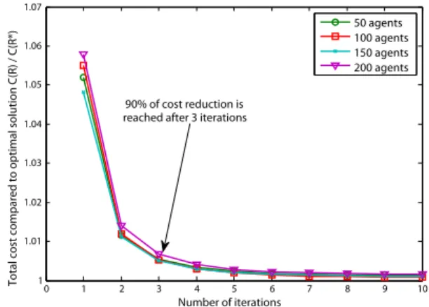
Simulation Results

In the previous section we proved the convergence of the introduced algorithm to the global optimal solution. Since we do not have a bound on the number of iterations needed for convergence, we conducted simulations on randomized data to get an indication of the convergence rate and scal-ability. In this section we present the results of our exper-iments. In our experiments we considered populations of up to 200 agents and varied the number of time slots up to 48. For the analysis we had to specify the market prices and the agents’ individual constraints. We based the prices on the pricing model of BC Hydro as in Figure (1) and generated the values for the prices uniformly distributed

pL

j ∈ [4,8], pLj ∈ [8,16] and hj = 10∗N, where N is the number of agents. We generated the constraints for

0 1 2 3 4 5 6 7 8 9 10 1 1.01 1.02 1.03 1.04 1.05 1.06 1.07 Number of iterations

Total cost compared to optimal solution C(R) / C(R*)

50 agents 100 agents 150 agents 200 agents 90% of cost reduction is

reached after 3 iterations

Figure 3: Reduction of total cost over the course of the algo-rithm for different agent populations sizes.

the lower and upper bounds and total consumption uni-formly distributed rij ∈ [6.5,11.5], rij ∈ [rij,2rij] and

τi ∈ h PM j=1rij,0.4 PM j=1rij+ 0.6 PM j=1rij i . Figure (3) illustrates the results of our experiments, showing how the total cost is reduced over the course of the algorithm. Since the agents have no individual virtual price signals in the first iteration, they optimize their cost according to the market prices. The graph shows the cost reduction for the different agent populations. Each data point is the average over all variations of numbers of time slots. The main finding is that over all experiments we see that90%of the cost reduction is reached within3iterations. The average cost reduction is

5.3%of the initial cost. Since the simulation was conducted only on randomized data, this cost reduction is just a first in-dication of possible gains. We plan to evaluate our approach on real consumption and pricing data in future work.

Conclusion

In this paper, we presented an iterative coordination algo-rithm to minimize the energy cost of a consumer coopera-tive given private information about the demand constraints. We designed a virtual price signal that coordinates the con-sumers’ demand shifts such that the total cost is reduced in each iteration. Then we proved the convergence of the algo-rithm to the global optimal solution. Finally our simulations indicate that the algorithm scales with the number of agents and consumption slots.

Future work will first check the individual rationality of an agent to join the cooperative and also the incentive com-patibility of an agent to report his consumption in each iter-ation truthfully. We will also look at scenarios with the pres-ence of storage and generation. The consumer group may have centralized and or decentralized generation and/or stor-age facilities. We also aim to consider uncertainty of prices. The electricity price is uncertain, when the planning horizon is longer than the horizon for which prices are known. More-over we may consider the setting of the coordinator being a profit making entity.

References

Boyd, S., and Vandenberghe, L. 2004.Convex optimization.

Cam-bridge university press.

Chu, C., and Jong, T. 2008. A novel direct air-conditioning

load control method. Power Systems, IEEE Transactions on

23(3):1356–1363.

Conejo, A.; Morales, J.; and Baringo, L. 2010. Real-time demand

response model.Smart Grid, IEEE Transactions on1(3):236–242.

Dietrich, K.; Latorre, J.; Olmos, L.; and Ramos, A. 2012. Demand response in an isolated system with high wind integration. Power

Systems, IEEE Transactions on27(1):20–29.

Jellings, C. W., and Chamberlin, J. H. 1993. Demand Side

Man-agement: Concepts and Methods. PennWell Books, Tulsa, OK.

Kim, T., and Poor, H. 2011. Scheduling power consumption with price uncertainty.Smart Grid, IEEE Transactions on2(3):519–527.

Kirschen, D. 2003. Demand-side view of electricity markets.

Power Systems, IEEE Transactions on18(2):520–527.

Medina, J.; Muller, N.; and Roytelman, I. 2010a. Demand re-sponse and distribution grid operations: Opportunities and

chal-lenges.Smart Grid, IEEE Transactions on1(2):193–198.

Medina, J.; Muller, N.; and Roytelman, I. 2010b. Demand re-sponse and distribution grid operations: Opportunities and

chal-lenges.Smart Grid, IEEE Transactions on1(2):193 –198.

Mohsenian-Rad, A., and Leon-Garcia, A. 2010. Optimal residen-tial load control with price prediction in real-time electricity pricing

environments.Smart Grid, IEEE Transactions on1(2):120–133.

Mohsenian-Rad, A.; Wong, V.; Jatskevich, J.; Schober, R.; and Leon-Garcia, A. 2010. Autonomous demand-side management based on game-theoretic energy consumption scheduling for the

future smart grid. Smart Grid, IEEE Transactions on1(3):320–

331.

Parvania, M., and Fotuhi-Firuzabad, M. 2010. Demand response

scheduling by stochastic scuc. Smart Grid, IEEE Transactions on

1(1):89–98.

Pedrasa, M.; Spooner, T.; and MacGill, I. 2010. Coordinated

scheduling of residential distributed energy resources to optimize

smart home energy services. Smart Grid, IEEE Transactions on

1(2):134–143.

Philpott, A., and Pettersen, E. 2006. Optimizing demand-side bids

in day-ahead electricity markets. Power Systems, IEEE

Transac-tions on21(2):488–498.

Rahimi, F., and Ipakchi, A. 2010. Demand response as a market

resource under the smart grid paradigm. IEEE Transactions on

Smart Grid1(1):82–88.

Ramchurn, S.; Vytelingum, P.; Rogers, A.; and Jennings, N. 2011. Agent-based control for decentralised demand side management in the smart grid.

Ramchurn, S.; Vytelingum, P.; Rogers, A.; and Jennings, N. 2012. Putting the ’smarts’ into the smart grid: A grand challenge for

arti-ficial intelligence.Communications of the ACM55(4):86–97.

Roozbehani, M.; Ohannessian, M.; Materassi, D.; and Dahleh, M. 2012. Load-shifting under perfect and partial information: Models, robust policies, and economic value.

Tanaka, K.; Uchida, K.; Ogimi, K.; Goya, T.; Yona, A.; Senjy, T.; Funabashi, T.; and Kim, C. 2011. Optimal operation by control-lable loads based on smart grid topology considering insolation forecasted error.Smart Grid, IEEE Transactions on2(3):438–444. Voice, T.; Vytelingum, P.; Ramchurn, S.; Rogers, A.; and Jennings, N. 2011. Decentralised control of micro-storage in the smart grid.

InAAAI Conference on Artificial Intelligence.

Wood, A., and Wollenberg, B. 1996. Power generation operation and control, john wiley & sons.New York.