Omer Baluch A Thesis in The Department of Computer Science
Presented in Partial Fullfilment of the Requirements for the Degree of Master of Computer Science at
Concordia University Montreal, Quebec, Canada
March 18, 2012
c
Entitled: A Framework for Soft Real-time Analysis in OLAP System. and submitted in partial fulfillment of the requirements for the degree of
Master of Computer Science
complies with the regulations of the University and meets the accepted standards with respect to originality and quality.
Signed by the final examining committee:
______________________________________ Chair Dr. Sabine Bergler ______________________________________ Examiner Dr. Gregory Butler ______________________________________ Examiner Dr. Brigitte Jaumard ______________________________________ Supervisor Dr. Todd Eavis Approved by ________________________________________________ Chair of Department or Graduate Program Director
________________________________________________ Dr. Robin A. L. Drew, Dean
Faculty of Engineering and Computer Science
Omer Baluch
OLAP systems are designed to quickly answer multi-dimensional queries against large data warehouse systems. Constructing data cubes and their associated indexes is time consuming and computationally expensive, and for this reason, data cubes are only refreshed periodically. Increasingly, organizations are demanding for both historical and predictive analysis based on the most current data. This trend has also placed the requirement on OLAP systems to merge updates at a much faster rate than before.
In this thesis, we propose a framework for OLAP systems that enables updates to be merged with data cubes in soft real-time. We apply a strategy of local partitioning of the data cube, and maintain a “hot” partition for each materialized view to merge update data. We augment this strategy by applying multi-core processing using the OpenMP library to accelerate data cube construction and query resolution.
Experiments using a data cube with 10,000,000 tuples and an update set of 100,000 tuples show that our framework achieves a 99% performance improvement updating the data cube, a 76% performance increase when constructing a new data cube, and a 72% performance increase when resolving a range query against a data cube with 1,000,000 tuples.
List of Tables viii
List of Figures ix
1 Introduction 1
1.1 Overview of Research . . . 4
1.1.1 Local Partitioning of the Data Cube . . . 4
1.1.2 Using a “hot” Partition for Fast Merging of Updates . . . 5
1.1.3 Using Multi-core Processing . . . 5
1.1.4 Replacing the Buffering Subsystem . . . 6
1.2 Thesis Organization . . . 6
2 Background 8 2.1 Introduction . . . 8
2.2 Data Warehousing . . . 9
2.3 OLAP . . . 11
2.4 Hilbert Space-filling Curve . . . 14
2.5 Hilbert Tuple Differential Coding (HTDC) . . . 16
2.6 Hilbert R-tree Indexing . . . 19
2.7 Data Partitioning . . . 21
2.8 Parallel Computing . . . 22
2.9 Parallel Programming Models . . . 24
3.2 Sidera Overview . . . 32
3.3 The Indexer . . . 34
3.4 Indexer Buffering Subsystem . . . 40
3.5 Indexer with Local Partitioning . . . 43
3.6 The Partition Table . . . 46
3.7 Tuple Distribution on a Shared-memory Architecture . . . 46
3.8 Merging Updates and the“hot” Partition . . . 47
3.9 Indexer with Multi-core Processing . . . 50
3.10 Query Engine . . . 53
3.11 Query with Partition . . . 58
3.12 Query Engine with Multi-core Processing . . . 59
4 Results 63 4.1 Hardware and Software Specifications . . . 63
4.2 Building and Updating the Datacube and Indexes . . . 64
4.2.1 Varying Number of Records . . . 65
4.2.2 Varying Number of Dimensions . . . 67
4.2.3 Varying Number of Threads . . . 69
4.2.4 Varying Number of Partitions . . . 71
4.2.5 Varying the Size of the “hot” Partition . . . 71
4.3 Query Engine . . . 75
4.3.1 Single Tuple Query . . . 75
4.3.2 Range Query . . . 76
5 Conclusions 82
5.1 Summary . . . 82 5.2 Future Work . . . 85
Bibliography 87
4.5 Indexer Build Run-times using Different Number of Threads. . . 69
4.6 Indexer Update Run-times using Different Number of Threads. . . 70
4.7 Indexer Build Run-times using Different Number of Initial Partitions. 71 4.8 Indexer Update Run-times using Different Number of Initial Partitions. 72 4.9 Non Multi-core Indexer Update Run-times using “hot” Partitions of Various Sizes. . . 73
4.10 Multi-core Indexer Update Run-times using “hot” Partitions of Various Sizes. . . 74
4.11 Query Engine - 1 Tuple Query. . . 76
4.12 Query Engine - Range Query. . . 77
4.13 Query Engine - Pathologically Large Query. . . 78
4.14 Query Engine - Packing vs. Striping - Run-times. . . 79
4.15 Query Engine - Packing vs. Striping - Disk Accesses. . . 80
4.16 Query Engine - Packing vs. Striping - Disk Seeks. . . 81
2.1 The Business Intelligence (BI) Architecture. . . 9
2.2 The Star Schema. . . 11
2.3 An OLAP Data Cube with 3 Dimensions. . . 12
2.4 Examples of Space Filling Curves. . . 15
2.5 First Four Orders of the Hilbert Curve. . . 16
2.6 First Four Orders of the Hilbert Curve. . . 18
2.7 The R-tree. . . 20
3.1 The Sidera Architecture. . . 33
3.2 Buffering Subsystem - Intermediate Files . . . 40
3.3 File Based Buffering Subsystem . . . 42
3.4 Bi-directional In-memory Subsystem . . . 44
3.5 Run-time by Stages for Indexer with Partitioning . . . 50
4.1 Indexer Run-times using Recordsets of Varying Number of Tuples. . . 67
4.2 Indexer Run-times using Recordsets with Varying Dimensions. . . 68
4.3 Indexer Run-times using Varying Number of Threads. . . 70
4.4 Indexer Run-times using Varying Number of Partitions. . . 72
4.5 Varying the Size of the “hot” Partition. . . 75
4.6 Query Returning a Single Tuple. . . 76
4.7 Range Query. . . 77
4.8 Pathologically Large Query. . . 79
4.9 Hilbert Packing vs. Hilbert Striping - Run-time. . . 80 ix
Introduction
Organizations all over the world are collecting data at an unprecedented pace and storing it in large databases. It is no longer unusual to hear of terabyte size databases, and there are documented examples of databases that have exceeded a petabyte [68]. As an example, in 2009, Yahoo! [3] reported having over 6 petabytes of data in their Everest system and expected to pass the 10 petabyte threshold by the end of that same year.
The data is collected from diverse sources such as retail sales transactions, online browsing activity, social networking sites, scientific research, or even sensors [6][26] [47]. Much of this data is managed and stored using an online transaction processing system (OLTP). Relational database management systems (RDBMS) [49] are an ex-ample of OLTP systems, and are primarily designed to handle a large volume of small transactions efficiently. The data collected by these systems is described asprimitive data because the main purpose of these systems is to keep a record of transactions, and not to analyze the collected data [43]. Current RDBMS are based primarily on the relational model described by Codd [14].
As the size of databases has grown over the years, organizations have been eager
because it is used to make management decisions, or to derive an answer to a question based on certain facts [43]. A few examples of DSS are Business Intelligence (BI) tools that include online analytical processing (OLAP) tools, data mining software, and expert systems.
A DW is considered to be a historical snapshot of the operational database, and is a separate entity from the operational database [49]. Traditionally, the data from the RDBMS was loaded into the DW either weekly or even nightly, usually when the RDBMS was offline. The reason for this is that the data needs to be transformed through a process called ETL (Extract-Transform-Load), so that data from hetero-geounous RDBMS sources is made uniform in the DW. Due to the high volume of data that needs to be transformed, the enormous burden on the operational database made it difficult to keep the RDBMS system online and at the same time upload the data into the DW [50].
OLAP systems are designed to quickly answer multi-dimensional queries against large DW systems. Based on the multidimensional data cube data structure [38], aggregrate values such as sum and averages are pre-computed using the data in the DW, and stored in the data cube. Users retrieve the values by locating the intersection of the specified dimensions. Constructing data cubes and their associated indexes is time consuming and computationally expensive [12]. For this reason, data cubes are only refreshed periodically.
Increasingly, organizations are demanding for both historical and predictive anal-ysis based on the most current data. In order to respond to this demand, DW tech-nologies have moved towards real time updates. Changes in the RDBMS are being pushed into the data warehouse at a much faster rate than before. Instead of weekly or even daily updates, changes from the transactional system are being continuously pushed into the data warehouse [5]. This trend has also placed the requirement on OLAP systems to merge updates at a much faster rate than before.
Sidera is a parallel OLAP server developed by Eavis that runs on a commodity cluster [29]. It exploits the clustering properties of the Hilbert space filling curve to achieve balanced data cube partitioning across the nodes in the cluster. Indexes are built using the R-tree data structure [28][40] and both the data and indexes are com-pressed using Hilbert Tuple Differential Coding(HTDC) [27]. The HTDC compression allows up to 90% compression of the distributed datacube, as well as up to 98% com-pression for the R-tree indexes [27]. Sidera also supports multi-dimensional caching, hierarchy-aware query resolution, and approximate query answering [30][31][32].
HTDC compression is a computationally expensive operation. Because complete materialized views must be decompressed before merging updates, the run-time for updating the data cube is almost as high as that for building the data cube. Query resolution times also suffer because blocks containing matching tuples must be de-compressed in order to retrieve the tuples. Thus, the information contained in the data cubes quickly looses its effectiveness because updates cannot be merged fast enough without affecting system performance and user experience.
In this thesis, we propose a modified architecture for the Sidera OLAP server that enables updates to be merged with the data cube in soft real-time. We apply
updates and therefore increase the frequency at which the data cube can be refreshed, while improving the run-times for building the data cubes and query resolution. As far as we know, no research has yet explored a local partitioning strategy and multi-core processing in an OLAP server that uses HTDC compression such as Sidera to achieve soft real-time updates.
The rest of this chapter provides an overview of the work done to implement soft-real time updates in Sidera, and explains how the thesis is organised.
1.1
Overview of Research
The research presented in this thesis focuses on the modifications done to the ar-chitecture of the Sidera OLAP server to allow it to merge updates in soft real-time. More specifically, the following changes were applied to the indexer and query engine, which are the two key components of Sidera that generate, update and query the data cube.
1.1.1
Local Partitioning of the Data Cube
We implemented local partitioning of the data cube and compressed each partition using HTDC compression. Each partition has an Linear Breath First (LBF) R-tree index [28] which is also compressed. A partition table is used to keep track of the number of partition per materialized view. We implemented the indexer to run on
a single node in order to obtain measurable results. We also used Hilbert packing to distribute the tuples across the partitions. This minimized the number of blocks retrieved from disk when resolving a user query.
1.1.2
Using a “hot” Partition for Fast Merging of Updates
For each materialized view, a “hot” partition is used to merge updates. As the “hot” partition reaches a certain size, it is capped and a new “hot” partition is started. Since merging updates is a computationally expensive operation, the “hot” partition was limited to a certain size. A side effect of merging updates with a “hot” partition is the introduction of duplicate tuples. For this reason, the query engine was modified to remove duplicate tuples and aggregate measures on the fly.1.1.3
Using Multi-core Processing
Exploiting the processing capabilities of multi-core processors, we implemented shared memory parallelism in both the indexer and the query engine to handle computation-ally expensive operations such as Hilbert conversions, compression and decompres-sion, and sorting. The OpenMP library was used to incrementally add multi-core processing to the Sidera code base.
An analysis of the Sidera codebase showed that certain time consuming operations consisted of a large number of manipulations of tuple data. Transformations such as converting multi-dimensional tuples to Hilbert indexes can be done independently from one another, which made them ideally suited for parallel processing. Using the pre-processor directives supplied by the OpenMP library, we divided these repetitive operatons into disjoint sets and distributed the work across multi-cores. The OpenMP library was also used to control the number of threads available to our system, as well
a series of intermediate files when converting data from one form such as multidi-mensional tuples to another form such as Hilbert indexes. This adds significant I/O overhead to both the indexer and the query engine, and coupled with overlapping I/O read and write calls, makes it difficult to parallelize on a single disk system.
We replaced the original file based buffering subsystem with an in-memory buffer-ing subsystem. Materialized views are read sequentially into memory, and all in-termediate transformations are done in memory and are fully parallelized. When the transformations are completed, the results are written back sequentially to disk, minimizing read and write calls, as well as the number of disk seeks.
1.2
Thesis Organization
The thesis is organized as follows
• Chapter 2 explains the key concepts behind the Sidera OLAP server as well data partitioning and multi-core processing. These will serve as a basis to understanding the ideas presented in the thesis.
• Chapter 3 begins with a brief overview of the Sidera architecture, followed by a more detailed description of the indexer and the query engine. For each component, we describe the original algorithms, and then describe the changes we made to achieve soft real-time updates. This includes implementing the local partitioning strategy, maintaining a “hot” partition for merging updates,
and adapting the query engine to aggregate duplicate records on the fly. The chapter also explains how we replaced the file based buffering subsystem with an in-memory based buffering subsystem, and how the indexer and the query engine were modifed to run on a single system with multiple multi-core CPUs.
• Chapter 4 describes the conditions under which we tested the modified archi-tecture and discusses the results we obtained by running the testcases.
• Chapter 5presents our conclusions based on the results we obtained in Chapter 4. We also provide a discussion on the limitations we encountered during our implementation, and suggestions for future work based on our research.
Decision support systems (DSS) have been around for several decades and are used to transform data into information with the eventual goal of supporting some type of decision making process within an organization.
Business Intelligence (BI) is a term used to describe a type of data-driven DSS that focuses on doing historical and predictive analysis of business data in order to support corporate decision making.
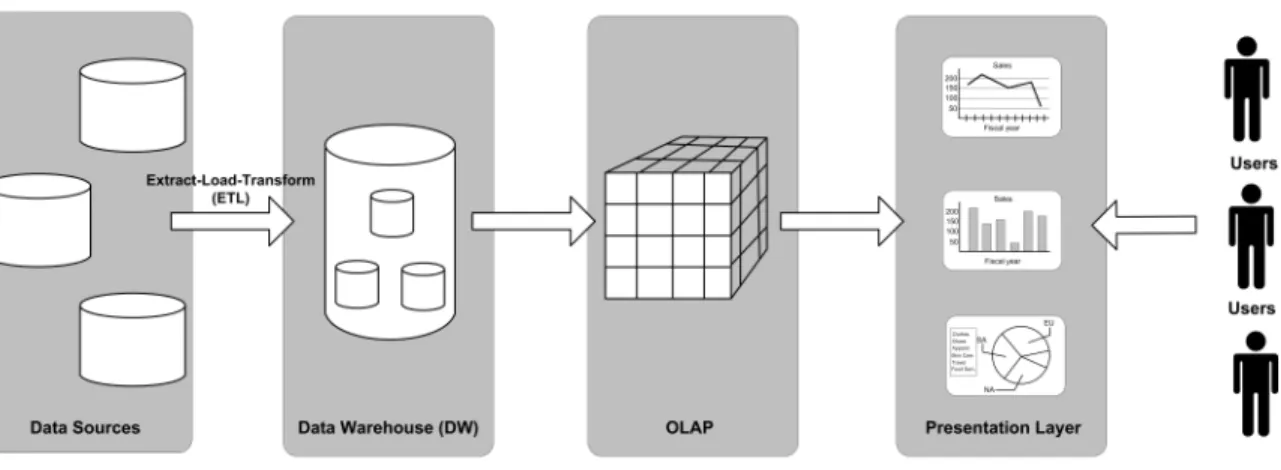
BI systems are assembled using several components that allow accurate and quick processing of large volumes of data, and presenting the results to the users in a timely and easy to understand fashion [20]. Central to the BI architecture are the data ware-house (DW), Online Analytical Processing (OLAP) tools, and the BI presentation layer. Figure 2.1 illustrates the BI architecture.
In a competitive world, making decisions based on the most recent available data has become increasingly important. There is a growing demand by organizations for BI tools that generate reports based on the most up-to-date operational data. In this thesis, we describe the modifications we made to an OLAP server that uses Hilbert
Figure 2.1: The Business Intelligence (BI) Architecture.
Tuple Differential Coding (HTDC) compression to enable updates to be merged in soft real-time without decreasing system performance.
The rest of this chapter presents the concepts necessary to understand the solution proposed in this thesis. We begin with a discussion on DW and OLAP, specifically maintaining OLAP data cubes. Next, we continue with a discussion on Hilbert space filling curves, Hilbert tuple differential coding (HTDC) compression, packed Hilbert r-trees, and data partitioning strategies. Finally, we provide an overview of parallel programming, multi-core programming and soft real-time systems.
2.2
Data Warehousing
Data warehouses (DW) are the foundation upon which many DSS are constructed. Primitive data from heterogenous Online Transactional Processing (OLTP) systems is collected, transformed and stored in a DW. Aside from BI tools, DW systems are also used by other DSS such as data mining tools and expert systems.
There are several reasons why BI tools do not execute directly using data from OLTP systems. The most important one is peformance. OLTP systems are designed primarily to handle a large volume of queries that affect a small number of records, whereas BI tools usually deal with a small number of queries that process a large volume of records or data [1]. Therefore, running BI queries against the OLTP systems result in degraged performance [12].
New data from the OLTP system is merged periodically with the DW. As the fact table becomes larger over time, merging new tuples and rebuilding indexes become increasingly expensive. For this reason, new data from the OLTP system is normally pushed into the DW only monthly, weekly or daily [48][64]. This implies that data in the DW never represents the most current data in the OLTP system, and users running reports on top of the DW warehouse using OLAP tools will almost never obtain information based on the most recent snapshot of the OLTP system. We say that the data in a traditional DW is stalewith regards to the OLTP system. Several strategies have been proposed to increase the update frequencies between the OLTP system and the DW.
Scheduling strategies have been proposed to minimize the DW staleness [37][5][36]. Scheduling algorithms trigger a refresh cycle when the fact table reaches a certain staleness threshold. Along the same lines, [51] mentions a strategy to track the staleness of the data in the DW with respect to the performance degradation if the
Figure 2.2: The Star Schema. DW was synchronized with the OLTP.
Others have looked at methods to allow updates to be incrementally merged with the DW while it remains online. In [63], using table replication and temporary tables was proposed to speed up merging update data.
Finally, another strategy is parallel DW. According to [48], the Extract-Transform-Load (ETL) process, which assembles data from heterogenous sources into the DW, consumes up to 70% of the processing time in a DW. In [70], the authors explain how the ETL process offers the possibility to implement both task and data parallelism and proceed to provide a framework for parallel ETL programming. Their results show that by investing a few more cpu cycles to implement their framework, it can significantly reduce the wall-clock time of an ETL process.
2.3
OLAP
Online analytical processing (OLAP) tools allow multi-dimensional queries against a DW to be answered quickly. This is done by pre-computing aggregates and storing
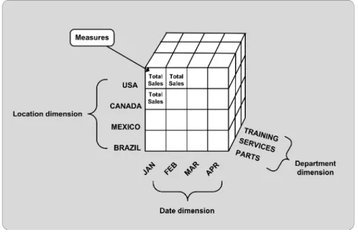
Figure 2.3: An OLAP Data Cube with 3 Dimensions.
the results in a data structure called thedata cube[38]. Figure 2.3 shows a data cube with 3 dimensions. Given that a fact table in a DW has d dimensions {A1,A2,A3, ... Ad}, then pre-computing the aggregate for every dimension combination results in
2d cuboids. Together, these cuboids constitute the data cube. We also refer to these
cuboids as materialized views, or simply as views.
User queries are resolved quickly by identifying the view that contains the pre-computed aggregate value for the specified dimensions and retrieving the value from the view. For a DW with a very large fact table, using a materialized view is faster than computing the aggregate values at query time.
OLAP tools have presented several challenges since their appearance. Data cubes require additional storage. For example, a DW fact table with 8 dimension tables will generate 28 = 1024 cuboids that must be stored on disk. Furthermore, certain dimension combinations produce views that are almost or even completely empty
leading to wasted storage space because space must still be allocated for these views [67].
Cube construction is also a computationally expensive and time consuming oper-ation. Like the DW, data cubes are traditionally refreshed monthly, weekly, or even daily, leading to the same staleness problem as in the DW.
An important component of OLAP servers are indexes, especially if the data cubes are stored on disk. R-trees or structures derived from the R-tree have emerged as a popular choice for multi-dimentional indexing [40][62][65][7][45][46][28]. We provide more details on a variation called the packed Hilbert R-tree data structure a little further in this chapter.
Parallel OLAP servers have been constructed on commodity clusters. These par-tition the data cube across the nodes in the cluster thereby distributing the work load among multiple machines [24][21][22][23]. Chen et al. [72][10][13] have demonstrated how large ROLAP data cubes can be constructed in parallel. These OLAP servers are built using a shared nothing parallel architecture because it has been shown to be more scalable compared to the more complexshared everything architecture. Fur-thermore, most of this research was done at a time when commodity computers were generally comprised of a one single core processor.
Other research has focused on strategies that minimize the number of materialized views that need to be constructed as well as the space required to store them on disk. Dehneet al. [25][23] have demonstrated that a partial data cube can be constructed and outlined parallel algorithms that reduced the cost of constructing the date cube from 20% to 70% compared to using naive methods. A partial data cube means that only a subset of the 2d materialized views need to be constructed and stored.
Cueva [27] have proposed a framework for compressing data cubes and their indexes using Hilbert Tuple Differential Coding (HTDC) compression, achieving compression rates of more that 90% for the data cubes, and up to 98% for their associated packed Hilbert R-tree indexes.
2.4
Hilbert Space-filling Curve
A space filling curve is a non-differentiable curve whose range [0,1] passes through every point in an N-dimensional space. It can also be described as a continuous, bijective function that maps every point from a unit interval [0,1] to a unique point in anN-dimensional unit hypercube [0,1]N. The first space filling curves were described by Giuseppe Piano and space-filling curves that map a unit interval to a 2-dimensional space [0,1]2 are known as Peano curves [59]. Peano curves are also fractals with a fractal dimension of 2.
We focus on two properties about space filling curves that are important to the material presented in this thesis. First, the transformation from a N-dimensional hyperspace to a space filling curve is said to apply a total order to the points in the hyperspace. This means that the transformation is reflexive, antisymmetric, transi-tive, and trichotomous.
Second, space filling curves preserve the locality of multi-dimensional points when they are mapped to the single dimension curve. This means that points that are
(a) Z-order Curve (b) Gray Code Curve (c) Hilbert Curve Figure 2.4: Examples of Space Filling Curves.
spacially close to each other in the N-dimension hypercube are mapped to points on the space filling curve that are close to each other. The level of clustering varies depending on the space filling curve [54].
There are many different space filling curves. Three important space filling curves are the Z-order curve [57], Gray code curve based on the Gray code [41], and the Hilbert curve [42]. An example of each are shown in Figure 2.4.
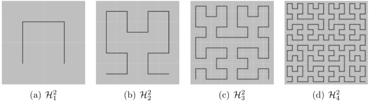
Among space filling curves, the Hilbert curve has been demonstrated to have superior clustering properties over other curves such as z-order and Gray code [44][54]. Moonet al. [54] provide the following notation 2.1 to describe successive iterations of Hilbert curves:
Hdk : [0,2kd−1]→[0,2k−1]d (2.1) wheredis the number of dimensions in the hyperspace andk denotes thekth-order
(or iteration) of the curve. Figure 2.5 shows the first four orders (or interations) of the Hilbert curve.
(a) H2 1 (b) H 2 2 (c) H 2 3 (d) H 2 4
Figure 2.5: First Four Orders of the Hilbert Curve.
curves are used to used to achieve block level compression for the OLAP data cube and indexes, and to construct R-tree indexes that minimize the number of disk blocks accessed during query resolution.
2.5
Hilbert Tuple Differential Coding (HTDC)
Hilbert tuple differential coding (HTDC) is a form of compression that is based on the Hilbert space curve that allows the data cube as well as the R-tree indexes to be compressed. This reduces the storage space required for both the data cube and the indexes.
HTDC relies on the total ordering imposed when points from a d-dimensional space is transformed to a Hibert space filling curve of length sd. It was described by
Eavis and Cueva [27], and it is a variation of the technique called Tuple Differential Coding described by Ng and Ravishankar [58]. The following is a summary of the technique.
Assume a relation R =< A1, A2, ..., Ad >, where Ai is a dimension with
car-dinality |Ai| for i = {1,2,3, ..., d}. R represents a multi-dimensional space where
the dimensions are used to specify the points in the space, and an individual tu-ple ϕ(a1, a2, ..., ad) is a point in the space. The transformation proposed by Ng and
Ravishankar imposes a lexicographic ordering to the tuples in R by the mapping function:
ϕ:R → NR (2.2)
where NR={0,1, ...,kRk −1}and kRk is defined as follows:
kRk= Yd i=1Ai :ϕ(a1, a2, ..., ad) = Xd i=1(ai d Y j=i+1 |Aj|) (2.3)
Once the tuples have been transformed to their ordinal values using the mapping function 2.2, the ordinals are sorted in ascending order. The compression process starts by storing the first ordinal in the first block, and then storing the differences between subsequent tuples. This is defined as the difference between tuples ϕi −
ϕi−1, where 0 < i ≤ |R|. The differences are saved in the block using run length
encoding (RLE). Since differences are small and require a small number of bits to encode them, Ng and Ravishankar have reported a 68% compression ratio. Note that the compression ratio for larger relations will be higher since the differences between tuples will be smaller, leading to smaller number of bits required to save the differences.
Eavis and Cueva proposed a similar technique, but where the mapping function applies a Hilbert order on the ordinals produced in the transformation stage. If we assume a space with d dimensions, we can transform it to
(a) H2 1 (b) H 2 2 (c) H 2 3
Figure 2.6: First Four Orders of the Hilbert Curve.
where a single multidimensional tuple ϕ(a1, a2, ..., ad) = CHIL(a1, a2, ..., ad).
Figure 2.6(a) shows a 2 dimensional Hilbert space where each dimension has a cardinality of 4. This space maps to 16 unique values on the Hilbert space filling curve. As an example, assume three tuples in the relation R with the tuples CHIL(1,2),
CHIL(1,4), CHIL(3,3). These are shows as points on the Figure 2.6(a).
The first step would be to transform the three tuples to a Hilbert ordinal. Again, looking at Figure 2.6(a),CHIL(1,2) maps to 4, CHIL(1,4) maps to 6, and CHIL(3,3)
maps to 9. After this, we sort the Hilbert ordinals in ascending order.
The first value stored in a compressed block will be 4. This is stored as a full integer value, requiring 32 bits on most platforms. For the next value, we calculate the differentρ= 6−4 = 2. Since we can express 2 as 10 in binary format, we remove all leading zeros and use only 2 bits to store the difference, saving 30 bits if we assume that an integer would require 32 bits. The next difference is calculated ρ= 9−6 = 3. Again, 3 is 11 in binary format, and we only need 2 bits and we save 30 bits. If we were to store multidimensional values, then we would need to store the (x,y) values of the coordinates, requiring 2 x 32 = 64 bits. So for the first tuple, which is stored
uncompressed, we save 32 bits since we only store one value. For the differences, we save 62 bits for each coordinate. Eavis and Cueva have reported compression ratios of more than 90% for data files, and up to 98% for the indexes.
Since the Hilbert transformation is a bijective function, compressed blocks can be decompressed to retrieve the original multidimensional tuples. Furthermore, since the first tuple in each disk block is stored uncompressed, decompression can be done at the block level. When resolving a user query, only the blocks containing tuples that satisfy the query parameters need to be retrieved and decompressed.
2.6
Hilbert R-tree Indexing
The R-tree structure was first proposed by Guttman [40] as a solution for indexing topological and cartological databases. The problem was that geographical loca-tions usually have at least two coordinates, and structures such as B-trees and ISAM indexes were inadequate because they ordered keys along a single dimensions. Multi-dimensional indexes such as Quad-tree [33], k-d trees [8], or the K-D-B tree [60] were also not sufficient because they either assumed a static database, which means that it was difficult to merge updates, or they performed poorly on range queries. The following is a quick overview of the R-tree.
In the R-tree, a leaf node is identified as (I, tuple-identif ier) wheretuple-identif ier is a pointer to an object stored the database, andI defines ad-dimensional bounding box that encloses the database object. We can also say that I = (I1, I2, ..., Id) where
Ii holds the maximum and minimum value of that object for the dimensioni.
Non-leaf nodes are constructed by adding entries in the form (I, child-pointer), where child-pointer is a pointer to either a leaf node, or to another non-leaf node.
(a) Bounding Boxes. (b) After Construction. Figure 2.7: The R-tree.
I defines the d-dimensional bounding box that encloses every bounding box in the child node.
Using Figure 2.7(a), we illustrate how an R-tree is constructed recursively from the leaf level up to the root node. Rectangles R8 to R19 are leaf-nodes and point to multidimensional tuples in the database. We start by constructing the non-leaf node R3, which encompasses nodes R8 and R9. We continue with node-leaf node R4, which encompasses nodes R10 and R11. We continue this process until we have grouped all the leaf level rectangles into the non-leaf rectangles R4 to R7. We repeat this process and regroup R3 to R5 inside R1, and nodes R6 and R7 inside R2. Finally, R1 and R2 are grouped inside the root node. Figure 2.7(b) shows the R-tree after construction. Searching for an object or a range of objects is accomplished using a depth-first search algorithm starting with the root node.
Starting with the assumption that most multidimensional databases are static, Rossopoulos and Leifker [62] provide a method for a “packed” R-tree so that there is minimal number of bounding box overlap and thus reduce dead-space. Instead of maintaining between m and M number of entries per non-leaf nodes, their method fills every node withM rectangle. This produces a very shallow but broad R-tree and
improves search queries. This is done without compromising the dynamic nature of R-tree.
Faloutsos and Kamel [45][46] push this idea further and first apply Hilbert ordering to the multidimensional database object before packing and constructing the R-tree. The clustering properties of the Hilbert space filling curve describe in Section 2.4 ensure that database objects that are spatially close together will be grouped in the same non-leaf node. They report better perfomance especially for skewed data distribution that better reflect real world situations.
The depth first search algorithms used for searching R-trees does not specify the order in which matching blocks are read from disk, and can lead to significant disk trashing due to high number of seeks. Eavis and Cueva [28] introduce the LBF R-tree in , including a linear breath first search (LBFS) algorithm that guarantees that blocks are read sequentially from a file, and degrades to a linear scan of the database in the worst case situation. Their algorithm minimizes the number of seeks a disk must perform, which is one of the major factors contributing disk latency. Accordingly, the LBF R-tree has been shown to reduce disk seeks by more than 50% compared to other R-trees.
2.7
Data Partitioning
Database partition has been a feature of many commercial databases such as IBM DB2 [16], Oracle [19] and SQL server [18]. Data partitioning means that the data in a database or even just a table is separated into different disjoint subtables. Parti-tioning tables helps manage the tables more easily and also speeds up performance in environments where the partitions can be manipulated in parallel.
in one single table, but a separate index is then built for each partition. Shard-ing is a technique where a database table is horizontally partitioned and each partition resides on a separate logical or physical server. Each server has a copy of the database schema, and no longer needs to be aware of the other servers.
• Vertical Partitioningbreaks tables into disjoint sets of columns, and each set is assigned to a subtable. The only column that is repeated in every subtable is the key column.
2.8
Parallel Computing
Parallel computing allows multiple program instructions to be executed simultane-ously on separate processing units. This is done by dividing instructions and data into discrete units and then distributing them across the processing units for execution. Parallel systems include various different architectures such as computers each with a single core processor connected together using a network, a single computer with multiple processors connected together by a bus, or a combination of both. More recent architectures also include processors that contain multiple processing units called cores in a single chip.
Physical limits such as power consumption and heat dissipation have placed a limit on the developement of single core processor architectures, leading processor manufacturers to switch to multi-core architures [17]. Cost per instructions is lower
for multi-core processors because they can execute more instructions at lower clock frequencies, which lowers the power consumption.
A common method of classifying parallel architectures is based on Flynn’s tax-onomy [35][34], which was introduced in the 1960s. It divides the architecture based on Instructions and Data, either of which can be Single or Multiple. Another com-mon method for classifying parallel architectures separates parallel systems into two distinct groups. The following is a brief description of the two groups.
• Shared-memory systems, which are also refered to as “shared-everything”
systems, have multiple processing units that access the same global address space and connect to the same memory using a shared bus. Any change to a memory location affects all processors. We also define shared-memory systems as having either Uniform Memory Access (UMA) or Non Uniform Memory Acess (NUMA), depending on how the memory is organized in the system. In the first case, each processor can access any memory location with the same latency. In the second, each processor can access certain memory locations faster than other locations.
An advantage of shared-memory systems is that data sharing is fast and uni-form. Disadvantages include problems with scalability because traffic on a shared bus ncreases geometrically with the number of processing cores. Cache coherency also adds complexity to this architecture because each processing unit has access to a private cache which is not always synchronized with the shared memory. When a processing carries out an instruction that affects a shared variable, another processing unit may attempt to change the same variable be-fore the cache value of the first processing unit is written back to memory. This
tems, have multiple processing units that each have access to their private global address space. The processing units must use a message passing proto-col to communicate with each other. This architecture is more scalable than shared-memory systems, and is easy to assemble using commodity off-the-shelf processors and an Ethernet network with TCP/IP for communications. An-other advantage of these systems is that there is no need to maintain cache coherency since each processor has exclusive access to its memory.
2.9
Parallel Programming Models
Modern processors implement techniques such as bit level and instruction level par-allelism that enable more instructions to be executed per clock cycle, but in order to take full advantage of a parallel computer system, developers must explicitely design their applications to run in parallel. There are two important types of parallelism.
• In task parallelism, separate tasks or functions can be executed on separate processing units. One of the challenges of task parallelism is how to distribute work evenly across processing units.
• In data parallelism, a large data set is partitioned into smaller disjoint sets such that each set can be processed independently from the other. These can then be distributed to separate processing units and the same instructions are carried on each disjoint set. An example would an operation on a matrix.
Designing and implementing parallel programs is difficult and often result in bugs that are difficult to detect because these bugs are related to thread timing. Program-mers must also manage access to shared resources (critical sections) and must also coordinate communication between the various executation cores. For this reason, several parallel programming models have been developed over the years to abstract many of the painful tasks when programming parallel applications.
• Shared-memory model (threads model)
In this model, the programmer is presented with a uniform memory model, although physical memory could be located on separate physical machines. Parallel execution is achieved by using threads which execute instructions in parallel. Threads access the same memory, and the programmer is responsible for ensuring that data is not corrupted or incorrect because of race conditions, and against deadlocks when using locks and semaphores. APIs built on this model are Posix threads [9], OpenMP [69], Unified Parallel C [71], X10 [15] and OpenCL [39].
• Message-passing model (distributed memory model)
In this model, the programmer is presented with a separate memory model for each processing unit, and the programmer must use a message passing protocol to exchange information between the processing units. The Message Passing Interface (MPI) API [53] is now the de-facto library used for message passing when developing applications for distributed memory systems. It is still the responsibility of the programmer to identify the parallel components, and to structure the application to run on parallel systems. In many cases, APIs such
Simply running a sequential application on a parallel system with pprocessing units does not always results inptimes speedup. The application must first be restructured so that instructions are distributed across the processing units. We define the speedup achieved as follows [52]:
Speedup = Execution time on 1 processor
Execution time on pprocessors (2.5)
The top part of the expression (2.5) represents the sequential execution time and the bottom part the parallel execution time. Under ideal conditions, we would like the parallel execution time to be equal to 1
p× sequential execution time. In other words,
we would like the speedup to be equal to p. This means that the more processor we allocate to the application, the faster it will execute.
Two factors limit the speedup we can achieve. The first factor is the ratio be-tween the time a program spends executing code that is inherently sequential, i.e. cannot be executed in parallel, and executing code that executes in parallel. The second factor that affects speedup is the the overhead associated with managing par-allel applications such as thread managements and communication between executing units.
application, Amdahl proposed an expression which is now known as Amdahl’s law [4]. After profiling an application, we defineS as the fraction of time it spends executing code that cannot be executed in parallel, and (1−S) as the fraction of time it spends executing code that can be execute in parallel. Then, Amdahl’s law defines speedup onp processors as follows:
Speedup = 1
S+ (1−pS) (2.6)
Amdahl’s law provides a close estimate to the speedup achieved when a parallel application is run on p processors. It can also be used to estimate an upper bound on the speedup that can be achieved. Assume an infinite number of processors are allocated to the application, then
Speedup = lim p→∞ 1 S+ (1−pS) = 1 S (2.7)
This means that the maximum speedup that can achieved when running an ap-plication on a parallel system is related to the fraction of time is spends running instructions that can only run sequentially.
2.11
Multi-core Programming
Back in 1965, Moore [56] predicted that the number of components in an integrated circuit roughly doubled every two years. This is known as Moore’s law, which states that the processing speed and the storage capacity of computer systems doubles every 18 months. Processor development has adhered to this trend by increasing the number
increasing performance, the focus shifted to multi-core cpu architectures. These are single chips with multiple executing units or core packed together. This has allowed the net number of intructions executed to be increased by executing them in parallel. The processor itself could run at a lower frequency, but the effective speed was the sum of the instructions run on all the cores.
There are several ways for a system to take advantage of the multiple cores avail-able. The first way is for the operating system to schedule a separate application to run on each core. For example, while a user is encoding video using one core, the virus scan application can run on the other core. In single core cpus, the operat-ing system would have to context switch and allocate a time slice for each of these applications. The other way is if an application process has multiple threads, then two or more threads can run on separate cores. But in order for this happen, it is up to the application to create the threads and ensure that resources are accessed appropriately. This means that the application developer must explicitely design the application to be multi-threaded.
2.12
OpenMP
OpenMP stands for Open Multi-Processing and it is a multi-platform shared mem-ory programming API that allows application developers to implement multi-threaded applications without directly using libraries such as Pthreads. In fact,
OpenMP use Pthreads behind the scenes, but abstracts a lot of details away from the user. This is done by providing the programmer with a set pre-precessor directives that allow multiple threads to be spawned when sections can be processed in parallel. There are also directives that allow to define shared variables and also the private variables for the separate threads. When a parallel section is completed, the API takes care of either removing the threads, or by returning them to the thread pool, where they can be recycled for another parallel section.
The API also provide contructs for declaring barriers and other synchronization points, as well as allowing the programmer to decide the number of threads to use. It follows a model where the main thread can fork multiple slave threads to do work on a parallel section before joining back to the main thread. This is a classic example of the fork-join model. Slave threads can either do the same work but each on a different part of the data (data parallelism), or each execute a separate task (task parallelism). OpenMP is used to parallelize code across multiple cores on a single cpu, or across multiple cpus but on a machine or a cluster that runs a single OS. It does not distribute work across independant machines, like MPI does. For this reason, it is not uncommon to see OpenMP used alongside MPI in many parallel and distributed applications.
OpenMP has many advantages over Pthreads. The API is much simpler and makes it easier to implement multi-threading without the complexity of Pthreads. The pre-processor directives can be added to non-multithreaded programs to convert them to multi-threaded programs without having to re-write the structure of the program. This is referred to incremental parallelism. When adding Pthreads to a non-parallel program, the structure must often be re-written. Platforms with non
2.13
Soft Real-time Updates
Real time computing consists of software and hardware that perform a task and can guarantee a certain deadline. We can define two different kinds of real-time computing, based on what happens if the deadline is not met.
Hard: if the deadline is not met, this leads to a system failure because the deadline is mission critical. As an example, certain critical subsystems in a nuclear plant must repond to changes within a determined period of time. Failure do so may lead to catastrophic results, and therefore deadlines are critical.
Soft: results are still useful after the deadline has been missed but not as useful as before the deadline, For example, a stock analysis program. The longer it takes to calculate the results, the price of the stock may rise or decrease and cause the investor to loose money.
In trying to implement any type of real-time application, it is important to un-derstand the deadlines, whether the application can continue if the deadline is not met, and what the results mean to the user if the deadline is not met.
Soft Real-time OLAP
3.1
Introduction
To achieve soft real-time OLAP, updates from the data warehouse must be merged with the data cube without taking the system offline or decreasing query resolution times.
This chapter describes a modifed architecture for the Sidera OLAP server that enables updates to be merged in soft real-time. Our architecture is designed to run on a single machine and exploits the multi-core architecture of newer systems for parallel processing. Our architecture is based on the design of the original Sidera OLAP server, but it has been adapted to run on a single machine, transitioning from adistributedarchitecture to ashared-memoryarchitecture. We will explain in Chapter 5 how our shared-memory version of Sidera could be incorporated with the original architecture to add multiple levels of parallelism to Sidera. Our modifications were done to the Sidera indexer and query engine.
We begin with a brief overview of the original Sidera architecture that uses Hilbert Tuple Differential Coding (HTDC) compression. This is followed by a description of
tribute processing loads across the available processor cores. The new architecture also replaces the older file based buffering subsystem with a faster in-memory based buffering subsystem, and introduces controlled I/O to ensure that files are read or written sequentially to minimize disk seeks.
We end the chapter with a description of the original Sidera query engine followed by the modified architecture. Distributing data across multiple partitions, as well as using a “hot” partition for merging updates puts an extra burden on the query engine. This is because updates are merged only with the tuples in the “hot” partition, which leads to potential duplicate tuples with respect to tuples that are in partitions other than the “hot” partition. For this reason, the query engine must be able to aggregate duplicate tuples on the fly without degrading query resolution times.
3.2
Sidera Overview
Sidera is a paralllel OLAP server that runs on a commodity cluster running the Linux operationg system. It is based on a distributed parallel architecture, where each node functions independently from the others. A Parallel Service Interface (PSI) layer is responsible for coordinating the activities between the nodes. The PSI is build using the standard Message Passing Interface (MPI) API, and abstracts much of the complexity in coordinating communcation between the nodes. Figure 3.1 from [29] shows an overview of the Sidera architecture.
Figure 3.1: The Sidera Architecture.
Each node in the cluster participates in sorting, compression, partitioning, distri-bution, indexing, and query resolution. Although one of the node is designated as the frontend node, its role is restricted to receiving queries from the user and forwarding them to the backend nodes. This eliminates bottlenecks that are often associated with parallel architectures that rely on a central node for process management.
Sidera uses a Hilbert space filling curve to partition data cubes and distributes them across the cluster. The Hilbert space filling curve has been shown to provide bet-ter locality-preservation in discrete multi-dimensional spaces than other space filling curves such as z-order or Gray code. For this reason, it is ideally suited for achieving optimal load balancing when partitioning data cubes across multiple nodes.
Coding (HTDC) compression that achieves almost 90% compression ratio [27]. Sidera also supports hierarchical representation, multi-dimensional query caching and approximate query answering.
Sidera follows a series of basic steps to transform and distribute the data cube across the cluster, and then to contruct the HTDC compressed views and indexes. Each step is carried out in parallel, with every backend node participating and using the PSI layer to coordinate the process.
Query resolution works with the same principle. Each backend node holds a par-tition of any given view, and participates in locating tuples that may match the query parameters. Using the PSI layer to coordinate the process, the backend nodes retrieve matching tuples and work together to merge their local results before returning the final result set to the frontend node.
3.3
The Indexer
The original Sidera indexer algorithm is divided into three stages. In the first stage, each backend node prepares a materialized view by converting the tuples into their corresponding Hilbert indexes and then sorting the view in ascending Hilbert order. In the second stage, the backend node stripes the view to create n partitions, where n is the number of backend nodes in the cluster. It then proceeds to send a partition
to every node including itself, and at the same time receives partitions of other ma-terialized views from the remaining backend nodes. In the third stage, each backend node creates a local HTDC compressed view using the partition it has received in stage two, and builds a compressed Hilbert R-tree index for that view. Stages one to three are repeated until every materialized view has been partitioned and distributed across the cluster.
Stages one and three do not require the PSI layer and run in parallel on each backend node, but stage two depends on the PSI layer to synchronize the distribution of partitions between the nodes. We will now use algorithm 1 to explain the three stages more in detail.
Lines 1 to 9 carry out setup work such as declaring certain variables required by the algorithm, as well as gathering some information about the cluster. We also use the PSI layer to determine which node in the cluster has the highest number of materialized views. This will determine how many times we will cycle through the main part of the algorithm.
Stage one starts at line 10 and runs until line 20. Here, variables required for coordinating the distribution are declared and assigned initial values. If this node has a materialized view to distribute in this round, the tuples are converted to Hilbert indexes, sorted in ascending order and partitioned. Although the calls to
ConvertToHilbertIndex(V[i]) and sortHilbertAscending(VH[i]) appear to
be both one step processes, they are built on the file based buffering subsystem used in the original Sidera architecture. We will elaborate more on the buffering subsystem in the next section, and explain how we replaced it with an in-memory subsystem to accelerate processing time.
2: VH ← minimal set of material views in Hilbert format. . empty at this point
3: viewCount← size(V)
4: viewCountList← empty list 5: maxV iewCount← 0
6: n← number of backend nodes in cluster 7: id← id for this node in the cluster
8: AllGather(viewCountList,viewCount,n) . through PSI layer get the
maxViewCount from every node into viewCountList 9: maxV iewCount← max(viewCountList)
10: for i= 1 →maxV iewCount do
11: toReceive ←false
12: toSend ←false
13: sendT o← 1 14: receiveF rom ←1
15: if i≤viewCount then . check if this node has something to send
16: VH[i]←convertToHilbertIndex(V[i])
17: sortHilbertAscending(VH[i])
18: VP ← getPartitions(VH[i])
19: toSend← true
20: end if
21: for j = 1→n do
22: send(toSend,sendT o) .through PSI layer
23: receive(toReceive,receiveF rom) .through PSI layer
24: if toSend== truethen
25: sendPartition(VP[j],sendT o) .through PSI layer
26: end if
27: if toReceive== truethen
28: buffer ← empty buffer to receive partition
29: buffer ← receivePartition(receiveF rom) .through PSI layer
30: createCompressedView(buffer)
31: buildCompressedIndex(buffer)
Algorithm 2Sidera Indexer (continued) 33: sentT o←(sendT o+ 1) mod n 34: receiveF rom←(receiveF rom−1) 35: if receiveF rom <1 then
36: receiveF rom←n 37: end if
38: end for 39: end for
Starting at line 21 until line 38, the partitions are distributed across the cluster. Although stage two is the distribution stage, stage three is overlapped with stage two with the compression and index building steps taking place on lines 30 and 31.
Although every backend node repeats lines 10 to 39 until all the materialized views have been distributed, not every node participates in sending and receiving. If a node has less materialized views to send as the maxV iewCount, then it does not send anything when it has processed all its views. Similarly, if a node is informed on line 23 that a node will not receive a partition, it simply loops to the next round.
On line 18, partitioning is achieved by striping the view such that node j will receive tuples (j, j +n, j + 2n, ...) where j is the node id and n is the number of nodes in the cluster. Because of the locality preservation property of the Hilbert space filling curve, tuples that satisfy the parameters of a range query along any dimension usually have corresponding Hilbert indexes that are close together on the Hilbert curve. This means that they are close together when Hilbert indexes are sorted in order. This Hilbert striping strategy therefore ensures that for any given range query, there is balanced distribution of work across the nodes in the cluster.
Algorithm 3 describes how updates are merged with the existing data cube. The process is similar to Algorithm 1. A minimal set of materialized views are generated
compressed R-tree indexes. 1: VU ←set of update views
2: VH ← set of views in Hilbert format. . empty at this point
3: viewCount← size(VU)
4: viewCountList← empty list 5: maxV iewCount← 0
6: n← number of backend nodes in cluster 7: id← id for this node in the cluster
8: AllGather(viewCountList,viewCount,n) . through PSI layer get the
maxViewCount from every node into viewCountList 9: maxV iewCount← max(viewCountList)
10: for i= 1 →maxV iewCount do
11: toReceive ←false
12: toSend ←false
13: sendT o← 1 14: receiveF rom ←1
15: if i≤viewCount then . check if this node has something to send 16: VH[i]←convertToHilbertIndex(VU[i])
17: sortHilbertAscending(VH[i])
18: VP ← getPartitions(VH[i])
19: toSend← true
20: end if
21: for j = 1→n do
22: send(toSend,sendT o) .through PSI layer
23: receive(toReceive,receiveF rom) .through PSI layer
24: if toSend== truethen
25: sendPartition(VP[j],sendT o) .through PSI layer
26: end if
27: if toReceive== truethen
28: buffer ← empty buffer to receive partition
29: buffer ← receivePartition(receiveF rom) .through PSI layer .
Algorithm 4Sidera Indexer - Updates (continued) 30: viewN ame← getViewName(buffer)
31: viewBuffer ← loadCompressedView(viewN ame) .decompresses
and loads stored view
32: mergeBuffer(viewBuffer,buffer) . mergesupdates in buffer into
viewBuffer
33: createCompressedView(viewBuffer)
34: buildCompressedIndex(viewBuffer)
35: end if
36: sentT o←(sendT o+ 1) mod n 37: receiveF rom←(receiveF rom−1) 38: if receiveF rom <1 then
39: receiveF rom←n 40: end if
41: end for
42: end for
that contain the aggregate values for the tuples in the update set, and these views are partitioned and distributed across the cluster. For each update view partition a backend node receives on line 29, the existing compressed view corresponding to that update view must be loaded, decompressed and the updates merged with it. This is reflected with three extra steps from line 30 to 32. Once the updates have been merges, the view is compressed again and the index is rebuilt. The important and time consuming property of the update algorithm is that the entire existing view must be loaded and decompressed, and the update tuples must be merged with it. Although materialized views are partitioned across the cluster, these partitions will reach a significant size over time and system performance will decrease when merging updates.
Eavis and Cueva [28] identify Hilbert sorting as the dominant cost in the construc-tion of the LBF R-tree, and since the size of the update set is much smaller than the size of the compressed view,|U| |rdata|, the cost of merging updates is much smaller
from their Hilbert index to multi-dimensional format, and this is a computationally expensive operation. In fact, all conversions between multi-dimensional tuples and their respective Hilbert indexes are expensive, and we describe later in this chapter how we leverage multi-core processing to reduce the processing time.
3.4
Indexer Buffering Subsystem
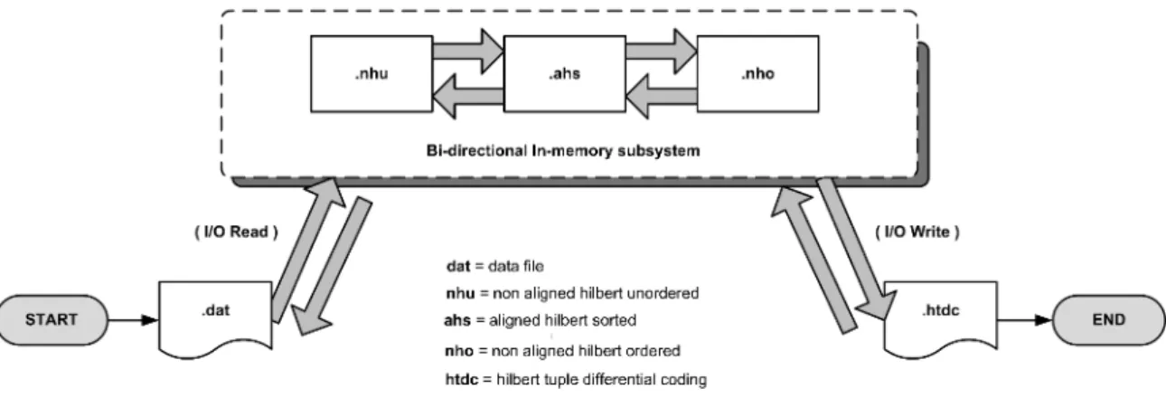
The original Sidera architecture uses a file based buffering subsystem, which allows it to stream data from large views on older systems that have restricted Random Access Memory (RAM). The process of converting a non compressed view to the final HTDC compressed view goes through several intermediate transformations. For each transformation, an intermediate file is generated, which becomes the input for the next transformation. Figure 3.2 shows the four major transformations that the file based buffering subsystem handles.
Figure 3.2: Buffering Subsystem - Intermediate Files
The first transformation consists of converting tuples with multi-dimensional co-ordinates in data file (.dat) into the non-aligned Hilbert unligned format (.nhu). The
(.nhu) file contains the tuples as Hilbert indexes, but they are not yet sorted. Next, we transform the tuples in (.nhu) format into aligned Hilbert sorted (.ahs) format. In this file, the tuples are sorted in ascending Hilbert order, and the Hilbert in-dexes are stored in a fixed byte format. The original Sidera system uses the GNU Multi-Precision (MP) library to handle and store Hilbert indexes. For high dimension spaces, primitive data types such as long may be too small to hold certain Hilbert indexes. Letdbe the number of dimensions in a hyper-space, andS is the largest car-dinality of any of the axis, then the length of the Hilbert space filling curve is defined as Sd. Essentially, this means that the size of the largest Hilbert index generated by
the transformation is Sd. If we take a view with six dimensions, and the cardinality
of the largest dimension is 5000. Then the highest possible Hilbert index that can be generate is 50006, and this number cannot be stored in along datatype.
The GNU MP library allows integers of arbitrary size to be stored and manipu-lated. It does this by allocating as many bytes as required to store an integer. This also means that Hilbert indexes stored in GNU MP data types may occupy different number of bytes in memory. The problem arises when the indexes are distributed across the cluster. The PSI layer is built on top of the Message Passing Interface (MPI) API, and requires data types in an array to be of fixed size. For this reason, the Hilbert indexes stored in GNU MP data types must first be transformed into fixed size data types. This is what the transformation from (.nhu) to (.ahs) does.
The transformation from (.ahs) to non-aligned Hilbert ordered (.nho) ordered converts the fixed size data types back to GNU MP data types. The only difference between the (.nhu) and the (.nho) is that the Hilbert indexes in the latter are sorted in ascending Hilbert order. Finally, the last transformation is from (.nho) to Hilbert
Figure 3.3: File Based Buffering Subsystem
tuple differential coding (.htdc) format, which is the format used by Sidera to store compressed materialized views. After the transformation from (.dat) format to (.htdc) has completed, the intermediate files are delete by the system.
Another way that the original file based buffering subsystem contributes to the Sidera indexer latency is by streaming data one block at a time. Figure 3.3 shows how tuples from the (.dat) file are transformed and stored stored in the (.nhu) format file.
A block is read from the first format, transformed and then written to the next format. This cycle is repeated until every block from the first format has been pro-cessed.
Although allowing older systems to process larger files sizes, the file based buffering subsystem also has a negative impact on the run-time. It forces the application to execute a large number of disk operations because (a) each block is individually read and written, requiring two I/O calls for each block, (b) it must create a series of
intermediate files and (c) reading from one file and directly writing to another file forces the disk to perform seek operations. These all contribute to increase the run-time of the original Sidera server.
In our modified architecture, we have replaced the file based buffering subsystem with a bi-directional in-memory subsystem. Figure 3.4 provides an abstract view of how this subsystem functions. For each materialized view, the view is first read sequentially from the (.dat) format into memory and all transformations take place in memory. At the end of the last transformation, the compressed view in (.htdc) format is written sequentially onto disk. All read and write calls are issued as a single call.
This approach reduces the number of I/O calls to a minimum and eliminates the disk seek operations incurred when overlapping I/O operations were issued for two separate files. Our subsystem can do transformations in both directions, making it also suitable for the Sidera query engine, which is explained a little further in this chapter.
3.5
Indexer with Local Partitioning
We now present a single process indexer for Sidera that locally partitions materialized views. Based on the original architecture of the Sidera indexer, it stores partitions on the same machine instead of distributing them across the cluster. We explain a little further in this chapter how we leverage multi-core processing to achieve parallel processing on a single machine. Effectively, our modifications transform Sidera from adistributed architecture to ashared-memory architecture. We propose in Chapter 5 a design to retro-fit this shared-memory version of Sidera into the originaldistributed
Figure 3.4: Bi-directional In-memory Subsystem
architecture to achieve multi-level parallelism in the Sidera OLAP server. Algorithm 5 presents the core algorithm of the indexer when the data cube is compressed and indexed.
From line 1 to 5, the algorithm prepares the necessary structures for processing. The number of partitions p can be any value such that p ≥ 1. In the distributed version of Sidera, the number of partitions was dependent on the number of nodes n in the cluster. In the shared-memory version, this is no longer the case.
Line 4 declares a buffer that is the in-memory subsystem described in Section 3.4. All transformation and partitioning tasks are performed by this structure. Another data structure, called the partition table is declared on line 5. The partition table stores information about each view, such as number of partitions, maximum partition size and if a “hot” partition exists on disk. At the end of the indexer process on line 15, the partition table is written to disk. This file will be used later by the indexer to
Algorithm 5Sidera Indexer with Local Partitioning
Require: Minimal set of materialized views on a single machine.
Ensure: Each view has been partitioned, compressed and has an Hilbert R-tree index.
1: V ← minimal set of materialized views 2: viewCount← size(V)
3: p←number of partitions to generate
4: BI ← in-memory subsystem . The in-memory subsystem takes care of
transformations and partitioning once the view is loaded
5: TP ←partition table . Holds information about views and partitions
6: for i= 1 →viewCount do 7: load(BI, V[i]) 8: VP ← getPartitions(BI) 9: for j = 1→p do 10: createCompressedView(VP[j]) 11: buildCompressedIndex(VP[j]) 12: updatePartitionTable(TP,VP) 13: end for 14: end for
R-tree index is build. The process is the same for every materialized view.
Finally, we note that I/O read calls are restricted to line 7 where the entire view file is loaded in one read operation, line 10 where the compressed view is written in one operation, line 12 where the compressed index is written in one operation, and line 15, when the partition table is written to disk.
3.6
The Partition Table
As mentioned in the previous section, the partition table is a simple structure that keeps tracks of materialized views, partitions, “hot” partitions, and the maximum size before capping a “hot” partition. The table is initially create and stored when the data cube is first generated, and it is updated by the update process. The query engine also relies on the partition table to determine how many partitions to query and whether it should search for a “hot” partition during query resolution.
3.7
Tuple Distribution on a Shared-memory
Ar-chitecture
In the distributed memory Sidera architecture, partitioning is achieved by striping the view such that node j will receive tuples (j, j +n, j + 2n, ...) where j is the node id andnis the number of nodes in the cluster. This is done to ensure that there is a balanced work distribution during query resolution. We refer to this as Hilbert
striping. In a shared-memory architecture, we are more interested in minimizing the number of blocks retrieved during query resolution. Once the blocks are loaded in memory, they can be distributed among the processing cores because each block is compressed at the block level and can be decompressed independently. Hilbert striping would make our architecture produce slower query times by spreading out the tuples in a range query across many blocks. For this reason, our shared-memory architecture compresses Hilbert indexes that are close together in the same block instead of striping them into different blocks. We refer to this strategy as Hilbert packing.
3.8
Merging Updates and the“hot” Partition
When merging updates, the modified architecture begins with a set of update views. Each update view is sequentially loaded in the in-memory buffer, and the tuples are converted to Hilbert indexes and sorted in ascending order. The algorithm then tries to locate the compressed “hot” partition corresponding to the update view. If a “hot” partition is found, it is loaded and decompressed. The Hilbert indexes of the update view are merged with those of the “hot” partition, and then they are re-compressed and saved to disk as the “hot” partition. If the number of the tuples in the “hot” partition exceeds the maximum allowed, the “hot” partition is capped with the maximum number of tuples, and the remaining tuples are stored in a new “hot” partition. If the indexer cannot find a “hot” partition, it simply starts a new one with the tuples in the update view. This is a repeated for every update view in the update set. Algorithm 6 shows how updates are merged with the “hot” partition in the Sidera indexer.